Simple Real-Space Picture of Nodeless and Nodal s-wave Gap Functions in Iron Pnictide Superconductors

Abstract

We propose a simple way to parameterize the gap function in iron pnictides. The key idea is to use orbital representation, not band representation, and to assume real-space short-range pairing. Our parameterization reproduces fairly well the structure of gap function obtained in microscopic calculation. At the same time the present parameterization is simple enough to obtain an intuitive picture and to develop a phenomenological theory. We also discuss simplification of the treatment of the superconducting state.

What is new in the iron pnictide[1] as a high-T_c superconducting material is its multi-orbital nature. Several microscopic calculations have been carried out to show that the five 3d orbitals of Fe atoms are entangled[2, 3] and that the superconducting gap function on the multiple Fermi surfaces are very complicated[4, 5, 6, 7, 8, 9]. Therefore, it is desirable to construct a description of the gap function, which is simple enough to obtain an intuitive picture for developing a phenomenological theory, but also which is powerful enough to capture its complicated multi-orbital nature. In fact, the gap functions of several kinds of iron-pnictide superconductors are not universal, i.e, nodeless in some materials and nodal in other materials[10, 11, 12, 13, 14, 15, 16, 17, 18]. Furthermore, there are some controversial results on the existence of inter-band sign reversal of the gap function. For instance, although quasi-particle interference measurements imply the existence of the inter-band sign reversal[19], robustness of T_c against impurity scattering suggests that there is no sign change between bands[20, 21]. Having these experimental situations in mind, we aim to construct a simple description of the gap function that enables us to discuss such complexity in a simple manner. We use orbital representation instead of band representation, and assume real-space short-range pairing. Our parameterization reproduces very well the structure of gap function obtained in microscopic RPA calculation. We also discuss simplification of the gap function for studying the superconducting state of iron pnictides.

We analyze the structure of the gap function based on the multi-orbital Hubbard model proposed by Kuroki et al.[3] that is downfolded from first-principle calculation. In this downfolding scheme, five bands around the Fermi energy are kept. The obtained five basis wave functions have the symmetry of Fe-3d orbitals, i.e., $d_{3z^{2}-r^{2}}$, $d_{zx}$, $d_{yz}$, $d_{x^{2}-y^{2}}$ and $d_{xy}$. One thing to be noted here is that the extended Brillouin zone is used, i.e, only one Fe atom is contained in a unit cell. We use the Hamiltonian $\mathcal{H}=\mathcal{H}_{0}+\mathcal{H}_{I}$ with

$$\mathcal{H}_{0}=\sum_{\bm{i},\bm{j},\sigma,ab}t_{a,b;\bm{i},\bm{j}}c^{\dagger}_{\bm{i}a\sigma}c_{\bm{j}b\sigma}=\sum_{\bm{k}\sigma,ab}\varepsilon_{ab}(\bm{k})c^{\dagger}_{\bm{k}a\sigma}c_{\bm{k}b\sigma},$$ (1)

where $t_{a,b;\bm{i},\bm{j}}$ is that obtained in the downfolding and $\mathcal{H}_{I}$ is the standard onsite multi-orbital interaction with $(U,U^{\prime},J_{H},J)$[22, 23]. In eq. (1), indices $a$ and $b$ run through 0 to 4, which correspond to $d_{3z^{2}-r^{2}}$, $d_{zx}$, $d_{yz}$, $d_{x^{2}-y^{2}}$ and $d_{xy}$ orbitals respectively. Details of the hopping integrals are different from system to system. In this paper, we mainly use the model with hopping integrals shown in Table I of Kuroki et al.[24], in which the hopping integrals up to the fifth-nearest neighbors are kept and the three dimensionality is neglected. We call this model as typical-1111 model in the following[25]. Full models for LaFeAsO, LaFePO and NdFeAsO are also used.

Before analyzing the gap functions, we discuss the orbital- and band-representations in the multi-orbital Hubbard model. The Hamiltonian, eq. (1), is written in the orbital representation and $\mathcal{H}_{0}$ can be diagonalized by a momentum-dependent unitary transformation. We call the transformed representation as band representation, in which the free Green’s function, $\hat{G}_{0}(k)$ (5$\times$5 matrix form, $k=(i\omega_{n},\bm{k})$), is diagonalized. However, since the momentum dependence of the unitary transformation is very severe in iron pnictides, the orbital character strongly depends on the Fermi surface positions. This causes the complexity when we use the band representation. In contrast, we find that the orbital representation is often suitable to discuss physics in real-space view. Although the Green’s function, $\hat{G}_{0}(k)$, in this representation has off-diagonal components connecting different orbitals, it does not make serious problems when we use the matrix form of Dyson-Gor’kov equation,

$$\begin{pmatrix}(\hat{G}^{0}(k))^{-1}&\hat{\Delta}_{\bm{k}}\\ \hat{\Delta}^{\dagger}_{\bm{k}}&-({}^{t}\hat{G}^{0}(-k))^{-1}\end{pmatrix}\begin{pmatrix}\hat{G}(k)&\hat{F}(k)\\ \hat{\bar{F}}(k)&-{}^{t}\hat{G}(-k)\end{pmatrix}=\hat{1},$$ (2)

which is in the present case, 10$\times$10 matrix. Note that we only consider the singlet channel and neglect the normal self-energy and frequency dependence of the gap function in eq. (2).

Now we begin to investigate the structure of $\hat{\Delta}_{\bm{k}}$. The key idea is to use the orbital representation and to consider in both real and momentum space. From now on, $\hat{\Delta}_{\bm{k}}$ is always in the orbital representation. First, we consider the diagonal elements of $\hat{\Delta}_{\bm{k}}$, i.e., the intra-orbital pairing in momentum space. Limiting our consideration to the s-wave channel, what is important is the gap value at $(0,0)$,$(\pi,0)$ and $(\pi,\pi)$ in the extended Brillouin zone, since the Fermi surfaces of iron pnictides are small and enclose those points. We denote the gap values on the orbital $i$ at $(0,0)$, $(\pi,0)$ and $(\pi,\pi)$ as $\Delta^{\Gamma}_{i}$, $\Delta^{M}_{i}$ and $\Delta^{\Gamma^{\prime}}_{i}$, respectively. For later use, we also define the difference of the gap value at $(\pm\pi/2,\pi/2)$ as $\Delta^{+}_{i}-\Delta^{-}_{i}$ (see Fig. 1(a)).

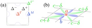
Figure 1: (Color online) (a) Schematic picture of the definition of $\Delta^{\Gamma}_{i}$, $\Delta^{M}_{i}$, $\Delta^{\Gamma^{\prime}}_{i}$ and $\Delta_{i}^{\pm}$. (b) Real space picture of the $\Delta_{ii}(\bm{k})$.

Now we move on to the real space picture. In order to make a simple description of the gap functions, we assume short-range pairings in the orbital representation. Then, $\Delta_{ii}(\bm{k})$ becomes

$$\Delta_{ii}(\bm{k})=a_{i}+2b_{i}(\cos k_{x}+\cos k_{y})+4c_{i}\cos k_{x}\cos k_{y}$$

$$+4\delta_{i}\sin k_{x}\sin k_{y},$$ (3)

where we have introduced three parameters, $a_{i}$, $b_{i}$ and $c_{i}$ representing on-site ($a_{i}$), nearest-neighbor ($b_{i}$), and next-nearest-neighbor ($c_{i}$) pairings. Anisotropy parameter $\delta_{i}$ is introduced for the $d_{zx}$ and $d_{yz}$ orbitals ($i=$1, 2), since they do not have 4-fold symmetry, i.e., we have $\delta_{1}=-\delta_{2}=\delta$ and $\delta_{0}=\delta_{3}=\delta_{4}=0$. Meanings of these parameters are described in Fig. 1(b). Relation between the parameters $(\Delta_{i}^{\Gamma},\Delta_{i}^{M},\Delta_{i}^{\Gamma^{\prime}},\Delta_{i}^{\pm})$ and $(a_{i},b_{i},c_{i},\delta_{i})$ can be simply written as

$$a_{i} = (\Delta_{i}^{\Gamma}+2\Delta_{i}^{M}+\Delta_{i}^{\Gamma^{\prime}})/4,\ b_{i}=(\Delta_{i}^{\Gamma}-\Delta_{i}^{\Gamma^{\prime}})/8,$$

$$c_{i} = (\Delta_{i}^{\Gamma}-2\Delta_{i}^{M}+\Delta_{i}^{\Gamma^{\prime}})/16,\ \delta_{i}=(\Delta_{i}^{-}-\Delta_{i}^{+})/8.$$ (4)

Note that the symmetry of 3d orbitals give $a_{1}=a_{2}$, $b_{1}=b_{2}$, $c_{1}=c_{2}$.

Next, we consider the off-diagonal elements of $\hat{\Delta}_{\bm{k}}$, i.e., inter-orbital pairings.

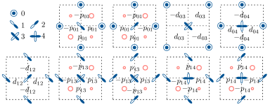
Figure 2: (Color online) Up left: Symmetries of the basis wave functions. Note that the coordinate of the original unit cell is used to describe the basis wave functions and they are rotated by $45^{\circ}$ from the usual definitions of the d-orbits on the square lattice. Others: Schematic real space pictures for the off-diagonal elements of $\hat{\Delta}(\bm{k})$. Red circle represents the As sites.

Assuming only the shortest possible pairing between the different orbitals (Fig. 2), we obtain

$$\Delta_{01}(\bm{k}) = 2ip_{01}(\sin k_{x}-\sin k_{y}),$$ (5a)

$$\Delta_{02}(\bm{k}) = -2ip_{01}(\sin k_{x}+\sin k_{y}),$$ (5b)

$$\Delta_{03}(\bm{k}) = 2d_{03}(\cos(k_{x}+k_{y})-\cos(k_{x}-k_{y})),$$ (5c)

$$\Delta_{04}(\bm{k}) = 2d_{04}(\cos k_{x}-\cos k_{y}),$$ (5d)

$$\Delta_{12}(\bm{k}) = 2d_{12}(\cos k_{x}-\cos k_{y}),$$ (5e)

$$\Delta_{13}(\bm{k}) = 2ip_{13}(\sin k_{x}-\sin k_{y}),$$ (5f)

$$\Delta_{23}(\bm{k}) = 2ip_{13}(\sin k_{x}+\sin k_{y}),$$ (5g)

$$\Delta_{14}(\bm{k}) = 2ip_{14}(\sin k_{x}+\sin k_{y}),$$ (5h)

$$\Delta_{24}(\bm{k}) = -2ip_{14}(\sin k_{x}-\sin k_{y}).$$ (5i)

Here the symmetries of orbitals are important for the sign of pairings as shown in Fig. 2. Furthermore, the matrix elements concerning $d_{zx}$ and $d_{yz}$ orbitals ($i=$1, 2) are determined by taking account of As atoms which exist above and below the Fe plane, because the $d_{zx}$/$d_{yz}$ orbitals are odd in z-direction and they do not have matrix elements with others without As. Characteristic feature found in eqs. (5) is that the off-diagonal elements have p-wave or d-wave symmetry. This is a direct consequence of the symmetry of the basis wave functions and the fact that the diagonal elements have s-wave symmetry. In the case where the diagonal elements have d-wave symmetry, we can do the similar analysis.

In order to determine the parameters in eqs.(3) and (5), we calculate the gap function $\hat{\Delta}^{\mathrm{RPA}}_{\bm{k}}$, by solving linearized Eliashberg equation with the effective interaction obtained within RPA. In this calculation, we follow the formalisms in Kuroki et al.[3]. We use the filling $n=6.1$, temperature $T=0.02$ eV and Coulomb parameters $(U,U^{\prime},J_{H},J)=(1.0,0.6,0.2,0.2)$ eV. The Brillouin zone is divided into 32$\times$32 meshes and 512 Matsubara frequencies are used. Then, using the gap function $\hat{\Delta}^{\mathrm{RPA}}_{\bm{k}}$, we obtain $(\Delta_{i}^{\Gamma},\Delta_{i}^{M},\Delta_{i}^{\Gamma^{\prime}},\Delta_{i}^{\pm})$ from which the parameters $(a_{i},b_{i},c_{i},\delta_{i})$ are determined through eqs. (4). Parameters $p_{ij}$ and $d_{ij}$ are determined from $\Delta_{ij}^{\mathrm{RPA}}(\bm{k})$ ($i\neq j$) similarly. The obtained results for a typical-1111 model are shown in Table. 1.

In Fig. 3, we compare the present simple description $\Delta_{11}(\bm{k})$, $\Delta_{33}(\bm{k})$ and $\Delta_{13}(\bm{k})$ with those in $\hat{\Delta}_{\bm{k}}^{\mathrm{RPA}}$ determined microscopically. We can see that our fitting is in good agreement with $\hat{\Delta}^{RPA}_{\bm{k}}$. Although some of the off-diagonal elements in $\hat{\Delta}(\bm{k})$ do not show a good coincidence, their magnitudes are small so that it does not lead to a serious problem. It is rather surprising that the gap function can be expressed only with the small number of parameters representing the real-space pairing up to next-nearest-neighbor. In contrast, when the gap functions are re-expressed in the band representation, they become very complicated for getting an intuitive picture.

Figure 3: (Color online) (a-c) Calculated $\Delta_{11}(\bm{k})$, $\Delta_{33}(\bm{k})$ and $\Delta_{13}(\bm{k})$ in RPA and fitted ones for typical-1111 model. (d) DOS for typical-1111 model calculated with 2048$\times$2048 k-space meshes.

Table 1: Parameters obtained in RPA calculation. Typical 6.1, typical 6.3 are the results for typical-1111 model with the filling $n=$6.1 and 6.3 respectively. The result for LaFePO is obtained with the filling $n=$6.1.

	$a_{1}$	$b_{1}$	$c_{1}$	$\delta$	$a_{3}$	$b_{3}$	$c_{3}$	$d_{12}$	$p_{13}$
typical 6.1	0.000746	-0.00382	-0.00155	0.000751	0.0213	0.0111	-0.00474	-0.000536	0.00446
typical 6.3	0.00185	-0.000598	-0.00517	0.000895	-0.00541	0.0117	0.000315	-0.000248	0.00642
LaFePO	0.00596	-0.00301	-0.00107	0.000504	-0.00716	0.00235	-0.000441	-0.00220	0.00166

In Fig. 3(d), we also plot the density of states (DOS) calculated with the fitted gap functions. The result shows nodeless two-gap behavior where the size of the smaller gap is about half of the larger gap.

We have checked the present parameterization for various cases to find that the fitting is very good for most of the cases. Exception is the case when we have too strong spin fluctuation on $d_{x^{2}-y^{2}}$ orbitals, for example in the model for NdFeAsO. In this case, $\Delta_{33}(k)$ has strong momentum dependence and eq. (3) is not enough to reproduce its strong momentum dependence. However, it is well known that the RPA estimation of the effective interaction gives stronger momentum dependence of $\hat{\Delta}(\bm{k})$ compared with other approximations. Therefore, we expect that the actual momentum dependence of $\Delta_{33}(\bm{k})$ in this case is much milder and the present parameterization works as well. In addition, the damping effect caused by impurities and the strong-correlation effects neglected in RPA generally give smoother gap functions.

In the following, we consider the possible simplification of the gap functions. For the typical-1111 model and the models for LaFeAsO and NdFeAsO[25], we expect that only $d_{zx}$/$d_{yz}$ and $d_{x^{2}-y^{2}}$ orbitals are necessary since they contribute most of the DOS near the Fermi energy. In this case, we need only parameters ($a_{1}$, $b_{1}$, $c_{1}$, $\delta$, $a_{3}$, $b_{3}$, $c_{3}$, $d_{12}$, $p_{13}$). We find that DOS calculated with keeping these parameters and setting others to zero can reproduce the DOS in Fig. 3(d). Furthermore, even if we assume $d_{12}=p_{12}=0$, the obtained DOS reproduces most of the features in Fig. 3(d), although there is a slightly different structure for the smaller gap. Since the resultant gap function is so simple, it is very useful to obtain an intuitive picture. Note that the above simplification can not be applied when $d_{3z^{2}-r^{2}}$ or $d_{xy}$ contribute to the DOS around Fermi energy, for example, in the case of LaFePO.

Next, we study the the difference between the nodal and nodeless s-wave gap in terms of the present parameterization. The existence of the nodal s-wave is theoretically predicted for the model for LaFePO[3]. Thus, we carried out similar calculation using the model of LaFePO. Here we use three-dimensional model and divide the Brillouin zone into 32$\times$32$\times$4 meshes. We find that the most significant difference from the typical-1111 model appears in $\Delta_{33}(\bm{k})$, which is shown in Fig 4 (see also Table. 1). Comparing Figs. 4 and 3, we can see that $\Delta_{33}(\bm{k})$ for LaFePO model has weaker momentum dependence than that for the typical-1111 model. In terms of our parameterization, $c_{3}$ is smaller in LaFePO. Due to this difference, $\Delta_{33}(\bm{k})$ at $(\pi,0)$ is positive in the typical-1111 model and negative in LaFePO. Note that $\Delta_{11}(\bm{k})$ at $(\pi,0)$ is positive for both models. Figure 4(b) shows the obtained DOS for LaFePO. We can see that (1) the partial DOS for the $d_{zx}$/$d_{yz}$ and $d_{x^{2}-y^{2}}$ orbitals show nodal behavior and (2) there is large remaining DOS in the gap around 20 meV since only a very small gap ($\lesssim$ 2 meV) appears in the $d_{3z^{2}-r^{2}}$ orbital.

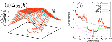
Figure 4: (Color online) (a) Calculated $\Delta_{33}(\bm{k})$ and fitted one for LaFePO model. (b) DOS for LaFePO model calculated with 512$\times$512$\times$32 k-space meshes.

To obtain a clear view on how the node evolves, we calculate DOS with a hypothetical gap function, with only $(a_{1},a_{3})=(\Delta,-\Delta)$. This means that we consider the totally momentum-independent s-wave gap in the orbital representation but with different sign on $d_{zx}/d_{yz}$ orbitals and $d_{x^{2}-y^{2}}$ orbitals. Interestingly, obtained DOS shows clear nodal behavior (Fig. 5(a)) although we input the gap function without any momentum dependence. This is because the orbital character varies along the positions of the Fermi surface. Some part of the Fermi surface enclosing $(\pi,0)$ has $d_{zx}/d_{yz}$ character and the gap function is $+\Delta$, while other part of that Fermi surface has $d_{x^{2}-y^{2}}$ character and the gap function is $-\Delta$. In this case, nodes appear on the Fermi surface. Although the gap with $(a_{1},a_{3})=(\Delta,-\Delta)$ is not the result of microscopic calculation, this argument captures the nature of the node obtained for LaFePO model. For comparison, we show the result with $(a_{1},a_{3})=(\Delta,\Delta)$ in Fig. 5(b). It shows clear full-gap feature and no nodal behavior as expected.

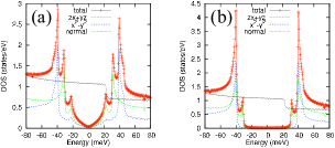
Figure 5: (Color online) DOS for the hypothetical gap function of $(a_{1},a_{3})=(\Delta,\Delta)$ (a) and $(\Delta,-\Delta)$ (b) calculated with 2048$\times$2048 k-space meshes and $\Delta=$40 meV.

Finally we investigate the doping dependence of the gap function within RPA calculation concentrating on the electron-doping side. We use the typical-1111 model and treat the doping as the rigid band shift. As we can see from Fig. 6, $\Delta_{33}(\bm{k})$ becomes flatter and flatter with doping. Figure 6(d) shows $a_{3}$, $b_{3}$ and $c_{3}$ in $\Delta_{33}(\bm{k})$ as a function of doping. The most important behavior is that of $c_{3}$. With doping the absolute value of $c_{3}$ becomes smaller and $c_{3}$ disappears around $n\sim 6.25$. Actually, the strongest superconducting instability channel changes from s-wave to d-wave around $n\sim 6.25$. (See the eigenvalues of the linearized Eliashberg equation for each channel $\lambda_{s}$ and $\lambda_{d}$ plotted in Fig. 6(d).) This suggests that the next-nearest-neighbor pairing of $d_{x^{2}-y^{2}}$ orbital plays important role in stabilizing s-wave channel. This is a good example to show the convenience of our parameterization in obtaining an intuitive picture for the gap function.

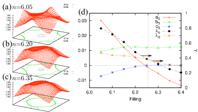
Figure 6: (Color online) (a-c) Doping dependence of $\Delta_{33}(\bm{k})$. (d) Doping dependence of $a_{3}$, $b_{3}$ and $c_{3}$. Eigenvalues of the linearized Eliashberg equation for s-wave pairing channel $\lambda_{s}$ and for d-wave pairing channel $\lambda_{d}$ are also plotted.

In summary we have investigated the structure of the gap function in iron pnictides. We have shown that the combination of the orbital representation and real space view leads to a powerful and convenient expression for the gap functions. This expression is powerful enough to reproduce the results of microscopic calculation and to discuss the variety of the gap functions. At the same time it is simple enough to make an intuitive picture and to calculate physical quantities in the superconducting state through eq. (2). Calculation of the physical quantities in this formalism should give interesting information on whether the gap function is s-wave or d-wave, or the gap function is s₊₊ or s_+-. Similar analysis on 122- and 11- system will also give important information.

References

- [1] K. Ishida, Y. Nakai, and H. Hosono: J. Phys. Soc. Jpn. 78 (2009) 062001.
- [2] D. Singh and M. Du: Phys. Rev. Lett. 100 (2008) 237003.
- [3] K. Kuroki, H. Usui, S. Onari, R. Arita, and H. Aoki: Phys. Rev. B 79 (2009) 224511.
- [4] Y. Yanagi, Y. Yamakawa, and Y. Ono: J. Phys. Soc. Jpn 77 (2008) 123701.
- [5] H. Ikeda: J. Phys. Soc. Jpn. 77 (2008) 123707.
- [6] Y. Fuseya, T. Kariyado, and M. Ogata: J. Phys. Soc. Jpn 78 (2009) 023703.
- [7] S. Graser, T. A. Maier, P. J. Hirschfeld, and D. J. Scalapino: New J. Phys. 11 (2009) 025016.
- [8] T. Nomura: J. Phys. Soc. Jpn. 78 (2009) 034716.
- [9] T. A. Maier, S. Graser, D. J. Scalapino, and P. J. Hirschfeld: Phys. Rev. B 79 (2009) 224510.
- [10] K. Hashimoto, M. Yamashita, S. Kasahara, Y. Senshu, N. Nakata, S. Tonegawa, K. Ikada, A. Serafin, A. Carrington, T. Terashima, H. Ikeda, T. Shibauchi, and Y. Matsuda: arXiv:0907.4399.
- [11] Y. Nakai, T. Iye, S. Kitagawa, K. Ishida, S. Kasahara, T. Shibauchi, Y. Matsuda, and T. Terashima: arXiv:0908.0625.
- [12] M. Hiraishi, R. Kadono, S. Takeshita, M. Miyazaki, A. Koda, H. Okabe, and J. Akimitsu: J. Phys. Soc. Jpn. (2009) 023710.
- [13] H. Fukazawa, Y. Yamada, K. Kondo, T. Saito, Y. Kohori, K. Kuga, Y. Matsumoto, S. Nakatsuji, H. Kito, P. M. Shirage, K. Kihou, N. Takeshita, C.-H. Lee, A. Iyo, and H. Eisaki: J. Phys. Soc. Jpn. 78 (2009) 083712.
- [14] M. Yashima, H. Nishimura, H. Mukuda, Y. Kitaoka, K. Miyazawa, P. M. Shirage, K. Kihou, H. Kito, H. Eisaki, and A. Iyo: J. Phys. Soc. Jpn. 78 (2009) 103702.
- [15] H. Ding, P. Richard, K. Nakayama, T. Sugawara, T. Arakane, Y. Sekiba, A. Takayama, S. Souma, T. Sato, T. Takahashi, Z. Wang, X. Dai, Z. Fang, G. F. Chen, J. L. Luo, and N. L. Wang: Europhys. Lett. 83 (2008) 47001.
- [16] T. Kondo, A. F. Santander-Syro, O. Copie, C. Liu, M. E. Tillman, E. D. Mun, J. Schmalian, S. L. Bud’ko, M. A. Tanatar, P. C. Canfield, and A. Kaminski: Phys. Rev. Lett. 101 (2008) 147003.
- [17] J. Fletcher, A. Serafin, L. Malone, J. Analytis, J. Chu, A. Erickson, I. Fisher, and A. Carrington: Phys. Rev. Lett. 102 (2009) 147001.
- [18] M. Yamashita, N. Nakata, Y. Senshu, S. Tonegawa, K. Ikada, K. Hashimoto, H. Sugawara, T. Shibauchi, and Y. Matsuda: arXiv:0906.0622 (2009) .
- [19] T. Hanaguri: private communication.
- [20] M. Sato, Y. Kobayashi, S. C. Lee, H. Takahashi, and Y. Miura: arXiv:0907.3007.
- [21] S. Onari and H. Kontani: arXiv:0906.2269.
- [22] M. Mochizuki, Y. Yanase, and M. Ogata: Phys. Rev. Lett. 94 (2005) 147005.
- [23] Y. Yanase, M. Mochizuki, and M. Ogata: J. Phys. Soc. Jpn. 74 (2005) 430.
- [24] K. Kuroki, S. Onari, R. Arita, H. Usui, Y. Tanaka, H. Kontani, and H. Aoki: Phys. Rev. Lett. 101 (2008) 087004.
- [25] Actually, this model gives a dispersion relation that is between LaFeAsO and NdFeAsO. Therefore, this ”typical–1111” model should be distinguished from the full model for LaFeAsO and NdFeAsO.