Reconstructing the Arches I: Constraining the Initial Conditions

Abstract

We have performed a series of $N$-body simulations to model the Arches cluster. Our aim is to find the best fitting model for the Arches cluster by comparing our simulations with observational data and to constrain the parameters for the initial conditions of the cluster. By neglecting the Galactic potential and stellar evolution, we are able to efficiently search through a large parameter space to determine e.g. the IMF, size, and mass of the cluster. We find, that the cluster’s observed present-day mass function can be well explained with an initial Salpeter IMF. The lower mass-limit of the IMF cannot be constrained well from our models. In our best models, the initial total mass down to a mass limit of $0.5\,{\rm M_{\odot}}$ is $(4.9\pm 0.8)\cdot 10^{4}\,{\rm M_{\odot}}$. The initial virial radius of the cluster is $0.77\pm 0.12\,\mathrm{pc}$. A concentration parameter of the initial King model $W_{0}=3$ gives the best results.

1 Introduction

The Arches cluster is one of only a few young and massive starburst clusters in the Milky Way. Its location at a projected distance of less than $30\,\mathrm{pc}$ from the Galactic centre and an age of only $\sim 2.5\,\mathrm{Myr}$ (Figer et al., 2002; Najarro et al., 2004) make this cluster a unique object for studying star formation and dynamical processes in the centre of galaxies (Portegies Zwart et al., 2010).

The observed present-day mass of the Arches cluster within $R=0.4\,\mathrm{pc}$ has been estimated with $\sim 1-2\cdot 10^{4}\,{\rm M_{\odot}}$ (Figer et al., 1999; Espinoza et al., 2009). With this mass a cluster will not survive long in the Galactic centre environment and evaporate on a time scale maybe as fast as $\sim 10\,\mathrm{Myr}$ (Kim et al., 1999; Portegies Zwart et al., 2002). The initial mass of the cluster has been determined from $N$-body simulations, however, different results have been obtained by different authors: Kim et al. (2000) found that their best model for the Arches cluster had a total mass of about $2\cdot 10^{4}\,{\rm M_{\odot}}$; Portegies Zwart et al. (2002), on the other hand, came to the conclusion that the cluster was initially more massive than $\sim 4\cdot 10^{4}\,{\rm M_{\odot}}$.

The initial mass function (IMF), a key aspect of star formation, seems to be uniform throughout the universe (Bastian et al., 2010). This universal IMF can be described by the power-law found by Salpeter (1955) for stars in the solar neighbourhood and is valid from $0.5\,{\rm M_{\odot}}$ to the highest masses. Below $0.5\,{\rm M_{\odot}}$, the IMF is significantly flattened (e.g. Kroupa, 2002).

Determining the IMF of young clusters from observations is not a straight-forward process. Uncertainties can arise from the measured luminosities, the estimated age of the cluster, the completeness of the observed sample, and the stellar evolution models. In addition, the non-linear dynamical evolution of the cluster has to be taken into account as shown in Fig. 1: as the star cluster evolves, more massive stars (star symbols) will move towards the cluster centre and low-mass stars (points) in the opposite direction (indicated by the arrows in the left image). If the detection of cluster members is radially limited (dashed circle), it will result in an observed mass function (MF) in the mass-segregated cluster (right image) that is different from the IMF. This effect is visualised in Fig. 1 by the ratio of low- to high-mass stars inside the dashed circles before and after mass segregation.

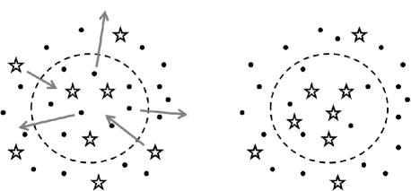
Figure 1: Schematic view on the cluster mass function and evolution. Low- and high-mass stars are shown by points and star symbols, respectively. The dashed circle indicates a radial observational limit. In the left image, the cluster is at $t=0$ with arrows denoting the effects of dynamical evolution. The right images shows the mass-segregated cluster.

In case of the Arches cluster, observations have revealed that the slope of the observed MF for $R\leq 0.4\,\mathrm{pc}$ is significantly flattened with $\Gamma\approx-0.9\pm 0.15$ with respect to the standard Salpeter IMF ($\Gamma=-1.35$) (Stolte et al., 2005, 2002; Figer et al., 1999), and therefore the Arches cluster has been regarded as a possible case against the universality of the IMF. More recently, however, Espinoza et al. (2009) derived a slope of $\Gamma=-1.1\pm 0.2$ in $R<0.4\,\mathrm{pc}$ and concluded that a standard Salpeter IMF cannot be ruled out for Arches. In addition to the radial variation in $A_{V}$, these authors also accounted for differential extinction variations, which can severely affect the incompleteness and may have biased the earlier results. Large uncertainties in the slope still remain, revealing the necessity to compare the observed cluster MF with simulations.

In addition to the flattened slope, there has been some debate whether the IMF of Arches is truncated at the low-mass end as the result of the extreme conditions at the Galactic centre where the cluster has formed. Possible evidence for a turn-over in the present-day MF was reported by Stolte et al. (2005), who determined a low- and intermediate-mass depleted MF in the cluster core ($R<0.2\,\mathrm{pc}$) with a turn-over at $6-7\,{\rm M_{\odot}}$. This truncation in the MF was not seen by Kim et al. (2006). They only found a local bump in the MF at $\sim 6\,{\rm M_{\odot}}$. Even if the MF is truncated at the low-mass end, it remains unclear whether this would be the result of a truncated IMF or a dynamical effect such as tidal stripping of low-mass stars.

With the aim to account for tidal stripping and mass loss in the Galactic centre potential, several studies have been done to determine the global IMF of the Arches cluster using numerical simulations, again coming to different conclusions: the model favoured by Kim et al. (2000) started with flat IMF with a slope of $\Gamma=-0.75$ close to the observed one. Portegies Zwart et al. (2002) found that the observed MF is the result of the dynamical evolution of the cluster and observational selection effects (namely radius-limited selection). They argue that the observed flat MF in the cluster core is therefore consistent with a global Salpeter IMF. The same effect is seen by Kim et al. (2006), however they suggest the slope of the IMF was $-1$ to $-1.1$, slightly shallower than Salpeter.

The Arches cluster also exhibits other clear signs of mass segregation. The slope of the observed MF for stars in different annuli changes with distance from the cluster centre. Towards the centre, the slope becomes shallower and further out the slope is closer to Salpeter (Kim et al., 2006; Stolte et al., 2005). Most recently, Espinoza et al. (2009) have reported $\Gamma=-0.9$ for $R<0.2\mathrm{pc}$ and $\Gamma=-1.3$ in the $0.2-0.4\mathrm{pc}$ annulus. Portegies Zwart et al. (2007) have found the same characteristics in numerical $N$-body models and concluded that the central flattening is the result of mass segregation. Furthermore, they claimed that the MF near the centre of the Arches cluster can be best described by a broken power-law, with a turning point at $5-6{\rm M_{\odot}}$ (at the position of the bump reported by Kim et al. (2006)). Based on these findings, they determined that the Arches cluster is about half-way to core collapse.

Despite the wealth of detailed observational data, large uncertainties regarding some of the properties of the Arches cluster remain, most importantly in the slope of the observed MF. Numerical simulations have been used to better understand the observations, but no fiducial model has emerged from these studies so far. In this paper, we want to expand previous numerical studies in order to reconstruct the initial properties of the Arches cluster. For this purpose, we have devised a new systematic method for comparing the results of $N$-body simulations with the present-day observations and apply this method to the Arches cluster. In addition to the mass function, our comparison method also considers the radial mass distribution, which has not been done previously. Another motivation for revisiting the Arches cluster is the recent determination of the cluster’s proper motion by Stolte et al. (2008). With this knowledge, the orbit of the cluster can be constraint, and a circular orbit used in some numerical studies (Kim et al., 2000; Portegies Zwart et al., 2002) can be ruled out.

In our $N$-body simulations, we model the Arches cluster on a star-by-star basis and, for the first time, systematically explore the parameter space to find the best set of initial conditions describing the Arches cluster. We vary parameters determining the initial mass, size, and concentration of the cluster. In addition, we also test which IMF can best explain the MF observed today. The total number of free parameters in our models is five, and a large number of simulations is required to search the full parameter space. Therefore, we decided to neglect the Galactic potential and stellar evolution for now. The aim of this paper is to introduce our comparison method and to constrain the initial conditions of the cluster. In a subsequent paper, we will use these results for simulations that include the here neglected processes. In particular, we will be able to extend the previous orbit analysis by Stolte et al. (2008), who employed a leap-frog integration of a point-mass cluster in a logarithmic potential. Our new models will provide additional constraints on the orbit based on the tidal effects on the cluster, which in turn will give us information about the birth place of the Arches cluster and its fate.

The initial conditions of the Arches cluster are of particular interest as the cluster was born in an extreme environment and is one of the few local examples of a star burst. NGC 3603 is the closest relative, with comparable central density and total mass, and with a similar observed top-heavy MF (Harayama et al., 2008). Quintuplet is another young massive cluster in the Galactic centre (Figer et al., 1999) and at an age of $\sim 4\,\mathrm{Myr}$ could be regarded as an older brother to Arches. The close location of Arches and Quintuplet suggest a prefered locus for the formation of these clusters within the central molecular zone. Insights on the formation locus would help us to understand the build-up of the inner bulge and the very massive, dense stellar population in the centre of the Galaxy. In addition, if cloud collisions are required to explain the dynamics of these clusters, this may limit the number of clusters capable of forming in the inner Galaxy, and may also be extrapolated to the central molecular rings of external galaxies.

The paper is outlined as follows: in Sec. 2, we describe the observational data we use. Then we explain the parameters for the cluster model in Sec. 3 and the simulations and their results in  4. We conclude and summarise in Sec. 5 and Sec. 6.

2 Observational data

We use data from observations by Stolte et al. (2005, NACO data hereafter). The NACO data has been taken using the ESO VLT AO system NAOS and the CONICA near-infrared camera in two wave bands, $H$ and $K_{s}$. The field of view is $\sim 25\arcsec$ squared or $1\,\mathrm{pc}^{2}$ (we assume a distance of $8\,\mathrm{kpc}$ to the cluster) with a resolution of $\sim 0.\arcsec 08$ or $0.003\,\mathrm{pc}$ at the distance of the Arches.

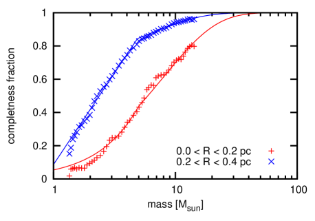
Figure 2: The completeness fraction in two radial bins as function of initial stellar mass. The data points (blue crosses and red pluses) are from the analysis of Stolte et al. (2005). The two full lines show a fit to the data.

The total data set consists of $\sim 2200$ stars belonging to the cluster and the field. In order to find the cluster stars, we apply the same colour selection as Stolte et al. (2005) (see their Fig. 2), retaining $\sim 1500$ cluster member candidates. We then fit the $K$-band magnitudes (corrected for the observed radial variation in extinction (Stolte et al., 2002)) against a $2.5\,\mathrm{Myr}$ Geneva main-sequence isochrone (Lejeune & Schaerer, 2001), assuming solar metallicity for Arches (Najarro et al., 2004). From this we get both present-day and initial stellar masses for each star in the sample. It should be noted, that the cluster age used here is different from the age used in Stolte et al. (2005) and therefore stellar masses have been re-derived for our preferred cluster age.

Because the incompleteness of the data due to crowding effects increases significantly for stars towards the low-mass end we reduced the sample further to about $300$ stars by selecting only massive stars with $m>10\,{\rm M_{\odot}}$. With our chosen lower mass limit, the data is 80% complete or better for any star mass and position, as a detailed analysis by Stolte et al. (2005) has shown. Fig. 2 shows the completeness fraction as a function of initial stellar mass for two different radial bins. We have fitted the results of Stolte et al. (2005, blue crosses and red pluses in Fig. 2) and also extrapolated for stellar masses above $\sim 15\,{\rm M_{\odot}}$. In the following analysis, we use this information to either correct the observational data or by randomly removing stars from our models. Note that only a few stars are added or removed by this correction for $m>10\,{\rm M_{\odot}}$.

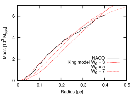
Figure 3: The cumulative mass profile for stars with $m>10\,{\rm M_{\odot}}$.

The field-of-view of the NACO data is such that only within a limited radius all stars of the cluster can be seen. This radius is $0.4\,\mathrm{pc}$ (see left panel in Fig. 11 which shows an image of all the $\sim 1500$ cluster stars; the radius of $0.4\,\mathrm{pc}$ is indicated by a circle centred on the centre of density). We therefore also limit our sample to the $234$ massive stars within this radius. The cumulative mass profile for these stars is shown in Fig. 3, where we also show the mass profiles for three different King models (King, 1966). All models have the same virial radius $R_{\mathrm{vir}}=0.5\,\mathrm{pc}$ and are scaled in mass to approximately fit the observed profile. The present-day profile of the Arches cluster is best described by a King model with $W_{0}=7$.

3 The model of the Arches cluster

In order to construct a model for the Arches cluster, we compare the results of $N$-body simulations with the observational data described above. The simulations start from a set of initial conditions with a number of parameters that can be varied to find the best fitting model. We have chosen the IMF, total mass, concentration, and size of the cluster as the free parameters. Other parameters are fixed: we assume an age of $2.5\,\mathrm{Myr}$ (see also Martins et al., 2008) and a distance of $8\,\mathrm{kpc}$ to the cluster.

3.1 Initial Mass Function

It has been discussed whether the IMF of the Arches cluster deviates from the norm, with a flattened distribution (for massive stars) with respect to a Salpeter IMF. Determining the IMF of a star cluster from its present-day mass function (PDMF) is not a straight-forward process as the PDMF is the result of stellar evolution and dynamical effects. Additional difficulties arise from observational limitations like crowding. In the following, we will use the observed MF for the comparison with our models. Since we do not take into account stellar evolution in our models, the observed MF is determined using the initial masses of stars (using the present-day masses of stars would change the MF only for stars with $m>50\,{\rm M_{\odot}}$). We also correct the observed MF for the incompleteness of the data. The observed MF can still differ from the underlying IMF due to the selection of stars inside $R<0.4\,\mathrm{pc}$.

In order to determine the slope of the observed MF, we use the sampled probability distribution $p(m)$, which is defined as a stepwise function through

$$p(m)=\frac{2}{N}\left(m_{i+1}-m_{i-1}\right)^{-1}\mathrm{for}\ m_{i-0.5}<m<m_{i+0.5}$$ (1)

where $m_{i}$ are the sorted initial stellar masses and $m_{i\pm 0.5}=0.5\cdot(m_{i}+m_{i\pm 1})$. In Fig. 4, we show $p(m_{i})$ for the NACO data, where we correct for the incompleteness of the data by dividing $p(m_{i})$ by the completeness fraction given in Fig. 2. The slope is derived by a least-square fit of power-law MF with two free parameters (normalisation and slope). This allows a more straight-forward fitting of the data than the commonly used mass binning. We find a shallow slope with $\Gamma=-0.94\pm 0.15$ for stars with $m>4\,{\rm M_{\odot}}$. Stolte (2003) has given an estimate of $\pm 0.15$ for the total error, which we also use here. The formal uncertainties of the fit are smaller (see Fig. 4), but these are not taking into account systematic uncertainties in determining stellar masses.

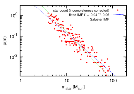
Figure 4: The sampled probability distribution $p(m)$ of the observed MF of stars with $m>4\,{\rm M_{\odot}}$ in the Arches cluster (red dots). The dotted blue line is a fitted power-law MF and the green dashed line is a Salpeter MF. Data is from Stolte et al. (2005) and corrected for incompleteness.

The slope we find here is in agreement with what has been reported by Stolte et al. (2005), and significantly deviates from a standard Salpeter MF. As a test, we have created random realizations of the Salpeter MF using $1\,{\rm M_{\odot}}$ and $120\,{\rm M_{\odot}}$ as the lower and upper mass limit, respectively. The total number of models was 1000 and each model consisted of 7500 stars which, on average, results in $320$ stars with $m>10\,{\rm M_{\odot}}$. We then fitted a power-law MF to each of the models in the same way we fitted the observed MF, using only the $\sim 320$ massive stars. In Fig. 5, we show the distribution of fitted $\Gamma$-values and from this distribution we derive $\Gamma=-1.35\pm 0.11$. The $\Gamma$-value derived from the observations is indicated by the shaded box. Based on this, only a small fraction of our models (nine) are consistent with the observed MF. However, given the uncertainties in deriving the initial masses of stars (which depend very much on the model for the rather unknown mass loss rate) and since so far any effects from the dynamical evolution of the cluster are not taken into account, we decided to use the slope of the IMF as a free parameter and studied, how a different IMF affects the present-day MF in the dynamically evolved and mass-segregated cluster. We also varied the lower mass limit of the IMF to test for a possible truncation of the IMF at lower masses.

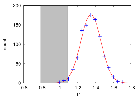
Figure 5: The distribution of fitted $\Gamma$-values of model MFs. Shown are the results from the models (blue pluses) together with a fitted Gaussian distribution. The observed MF slope is indicated by the shaded area.

3.2 Initial mass of the cluster

The choice of an IMF is also important for determining the total mass of the cluster. The present day mass of the cluster within $R=0.4\,\mathrm{pc}$ is $\sim 1-2\cdot 10^{4}\,{\rm M_{\odot}}$ (Figer et al., 2002; Stolte et al., 2008; Espinoza et al., 2009). Kim et al. (2000) estimate that Arches could have lost about half its initial mass due to its dynamical evolution in the Galactic centre, which would give an initial mass of $\sim 3\cdot 10^{4}\,{\rm M_{\odot}}$. On the other hand, Figer et al. (2002) calculated an upper mass limit of $7\cdot 10^{4}\,{\rm M_{\odot}}$ for the cluster, based on the virial theorem and the observed upper limit to the velocity dispersion of $22\,{\rm\,km\,s^{-1}}$ from radial velocities.

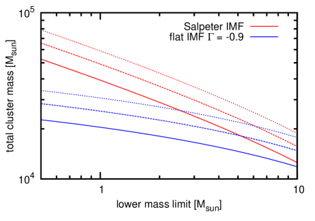
Figure 6: The initial mass of the cluster as a function of the lower mass-limit of the IMF for different IMFs. The three lines show different normalisations.

In Fig. 6, we show the initial cluster mass we derive for different IMFs. For each IMF we used three different normalisations such that the total number $N_{\mathrm{MS}}$ of star more massive than $20\,{\rm M_{\odot}}$ is $200$, $250$, and $300$. We then varied the lower mass limit of the IMF as it may be truncated in the Arches cluster (Stolte et al., 2005; Kim et al., 2006).

We find, that the total cluster mass can be initially as high as $\sim 8\cdot 10^{4}\,{\rm M_{\odot}}$ (Salpeter IMF and $N_{\mathrm{MS}}=300$) or even higher if stars below $0.5\,{\rm M_{\odot}}$ have formed in the cluster. For a flat IMF ($\Gamma=-0.9$), the total cluster mass does not depend much on the lower cut-off. The average mass ($N_{\mathrm{MS}}=250$) is about $\sim 3\cdot 10^{4}\,{\rm M_{\odot}}$ and a minimum initial mass of $\sim 2\cdot 10^{4}\,{\rm M_{\odot}}$ for $N_{\mathrm{MS}}=200$ is found, both in very good agreement with the findings of Kim et al. (2000); Kim et al. (2006).

3.3 Size of the cluster

The Arches is a very dense cluster with a central mass density of $\sim 2\cdot 10^{5}\,{\rm M_{\odot}}\,\mathrm{pc}^{-3}$ (Espinoza et al., 2009). The tidal radius of the Arches cluster is $\sim 1\,\mathrm{pc}$ and we determine the core radius with $r_{\mathrm{core}}=0.25\,\mathrm{pc}$ using all stars and with $r_{\mathrm{core}}=0.14\,\mathrm{pc}$ for stars with $m>10\,{\rm M_{\odot}}$. Following Casertano & Hut (1985), the core radius is defined throughout this paper as the density-weighted average distance of stars to the density centre.

The current concentration of the Arches cluster may be the result of its dynamical evolution as the cluster is probably evolving towards core collapse. We therefore use the initial concentration, parameterised in the King model concentration parameter $W_{0}$, and size of the cluster, namely its virial radius, as two more free parameter. The virial radius $R_{\mathrm{vir}}$ is defined as

$$R_{\mathrm{vir}}=\frac{1}{2}\frac{GM^{2}}{\left|U\right|}$$ (2)

with the gravitational constant $G$, the mass $M$ and potential energy $U$ of the cluster. Since $U$ cannot be observed, it may be more practical to know that the virial radius is proportional to the half mass radius.

3.4 Summary of model parameters

To summarise, the initial conditions for our cluster models are set by the virial radius, slope and low-mass cutoff of the IMF, concentration, and number of massive stars, which are varied systematically (see Tab. 1 below and Sec. 4.1).

4 Setup and results of simulations

Our aim is to find a numerical model of the Arches cluster that can explain the observed properties of the cluster. In this paper, we neglect the effects of the Galactic potential as well as stellar evolution. This allows us to perform a large number of simulations in order to constrain some of the parameters of our models. The simulations were carried out in the Starlab environment using the integrator kira (Portegies Zwart et al., 2001). GPUs, graphical processing units, were used to accelerate the calculations via the Sapporo library (Gaburov et al., 2009).

4.1 Initial conditions

Table 1: List of models.

Model	$W_{0}$	IMF	$m_{\rm low}$	$M_{\rm cluster}$	$N_{\rm cluster}$	$N(m>10\,{\rm M_{\odot}})$	parameter
			$[{\rm M_{\odot}}]$	$[10^{3}{\rm M_{\odot}}]$	$[10^{3}]$		$R_{\rm vir}[\mathrm{pc}]$	$N_{\mathrm{MS}}$
IKW03F05	3	flat	0.5	22.9	6.9	423	0.1 – 1.0	100 – 300
IKW03F10	3	flat	1.0	20.5	3.7	421	0.1 – 1.0	100 – 300
IKW03S05	3	Salpeter	0.5	52.7	31.9	552	0.1 – 1.0	100 – 300
IKW03S10	3	Salpeter	1.0	39.7	12.5	552	0.1 – 1.0	100 – 300
IKW03S40	3	Salpeter	4.0	20.6	1.9	540	0.1 – 1.0	100 – 300
IKW05F05	5	flat	0.5	22.7	6.9	413	0.1 – 1.0	100 – 300
IKW05F10	5	flat	1.0	20.2	3.7	413	0.1 – 1.0	100 – 300
IKW05S10	5	Salpeter	1.0	39.0	12.5	545	0.1 – 1.0	100 – 300
IKW05S40	5	Salpeter	4.0	20.8	1.9	543	0.1 – 1.0	100 – 300
IKW07F05	7	flat	0.5	22.9	6.9	422	0.1 – 1.0	100 – 300
IKW07F10	7	flat	1.0	20.7	3.7	421	0.1 – 1.0	100 – 300
IKW07S10	7	Salpeter	1.0	39.2	12.5	537	0.1 – 1.0	100 – 300
IKW07S40	7	Salpeter	4.0	20.8	1.9	551	0.1 – 1.0	100 – 300

Columns are: 1) model name; 2) the dimensionless King concentration parameter $W_{0}$ 3) the IMF used, where flat and Salpeter refer to power-law IMFs with $\Gamma=-0.9$ and $\Gamma=-1.35$, respectively; 4) lower IMF mass limit in ${\rm M_{\odot}}$; 5) total cluster mass in $10^{3}\,{\rm M_{\odot}}$; 6) total number of stars in the cluster in $10^{3}$; 7) total number of massive stars ($m>10\,{\rm M_{\odot}}$); 8) additional model parameter (virial radius $R_{\mathrm{vir}}$ and number of massive stars $N_{\mathrm{MS}}$) and their ranges

We use King models (King, 1966) in virial equilibrium as our initial cluster model. As the initial concentration of the cluster is not known, it is possible that the cluster has evolved to its current compactness from a less concentrated model. We therefore decided to use three different values for the initial concentration parameter $W_{0}$. For each concentration parameter we also tested both the Salpeter IMF and an IMF with a flat slope of $\Gamma=-0.9$. Furthermore, we also varied the lower mass limit of the IMF between $0.5\,{\rm M_{\odot}}$ and $4\,{\rm M_{\odot}}$. In total, we used 13 different sets of initial conditions for the cluster (see Tab. 1).

In addition, we also varied two free parameters for each of these models: the initial virial radius as $R_{\mathrm{vir}}$ and the initial number $N_{\mathrm{MS}}$ of stars with $m>20\,{\rm M_{\odot}}$. The latter is used to normalise the total cluster mass and we used five different values for $N_{\mathrm{MS}}$ between $100$ and $300$ in steps of $50$. This range covers the $127$ stars with $m>20\,{\rm M_{\odot}}$ found in the NACO data and the $\sim 200$ stars reported by Figer et al. (2002), also taking into account that a significant fraction of massive stars may no longer be bound to the cluster or is not observed. The differences between the two data sets can be explained by a different field-of-view ($25\arcsec$ squared in the case of NACO as compared to $40\arcsec$ squared for NICMOS) and the applied selection criteria to determine cluster membership. Varying $N_{\mathrm{MS}}$ increases the total number of models tested to $65$.

Our $N$-body simulations are in scale-free $N$-body units because we neglect stellar evolution and the tidal field. In $N$-body units, the gravitational constant $G$, the total mass of the system, and the virial radius are all set to unity (Heggie & Mathieu, 1986). The connection between the scale-free $N$-body units and physical units is then given by

$$G=1\frac{\mathrm{U}_{\mathrm{l}}^{3}}{\mathrm{U}_{\mathrm{m}}\mathrm{U}_{\mathrm{t}}^{2}}=0.0045\frac{\mathrm{pc}^{3}}{{\rm M_{\odot}}\mathrm{Myr}^{2}},$$ (3)

where $\mathrm{U}_{\mathrm{l}}$, $\mathrm{U}_{\mathrm{m}}$, and $\mathrm{U}_{\mathrm{t}}$ are the $N$-body units for length, mass, and time, respectively. The mass unit $\mathrm{U}_{\mathrm{m}}$ is naturally given by the total mass of the Arches cluster $M_{\mathrm{Arches}}$. A choice of $R_{\mathrm{vir}}$ defines $\mathrm{U}_{\mathrm{l}}$, which in turn determines $\mathrm{U}_{\mathrm{t}}$ via Eq. 3. The age of the cluster is $t=2.5\,\mathrm{Myr}$ or according to Eq. 3

$$t=\frac{2.5\,\mathrm{Myr}}{\mathrm{U}_{\mathrm{t}}}=2.5\cdot\sqrt{0.0045\frac{M_{\mathrm{Arches}}}{{\rm M_{\odot}}}\left(\frac{R_{\mathrm{vir}}}{\mathrm{pc}}\right)^{-3}}$$ (4)

in the dimensionless $N$-body time unit.

The virial radius was varied between $0.1$ and $1\,\mathrm{pc}$ in steps of $0.05\,\mathrm{pc}$. However, instead of increasing the number of models by another factor of 19, we make use of the scale-free nature of our simulations. For each value of $R_{\mathrm{vir}}$, the cluster has to be evolved to a different $N$-body time unit given by Eq. 4 to reach an age of $2.5\,\mathrm{Myr}$ in physical units. The $N$-body times to match the desired values of $R_{\mathrm{vir}}$ can be computed at the start of the simulation, and then snapshots are written at these $N$-body times during these simulations. Each of the snapshots corresponds to a snapshot of the Arches cluster at $t=2.5\,\mathrm{Myr}$ with a different $R_{\mathrm{vir}}$.

Each of the $65$ models was created ten times with a different random realization, so that a total of $650$ simulations were performed. However, once the simulations were finished, we averaged the global properties of each model before comparing them with the observations. We also took into account the incompleteness of the observations by randomly removing a few stars from our models according to the incompleteness tests depicted in Fig. 2. However, this has only little effect on the overall results as we already constrained our data sample to stars that are almost complete in the observations. In the end, we compared more than 1,200 simulation snapshots with the observations.

4.2 Comparing models and observation

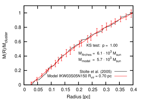
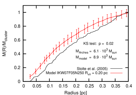
Figure 7: Comparing the normalised cumulative mass profile of model and observation. The red line shows the model data, with error bars indicating the standard deviation from averaging over ten random realization of the same model. The black line the observation and $M_{\mathrm{Arches}}$ is the total observed cluster mass for $m>10\,{\rm M_{\odot}}$ and $R\leq 0.4\,\mathrm{pc}$. Two different models are shown.

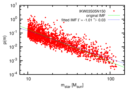
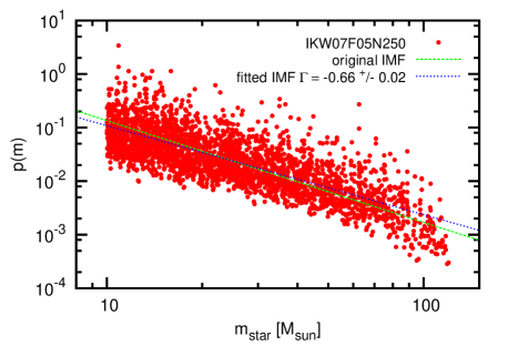
Figure 8: Determination of the model MF for $R\leq 0.4\,\mathrm{pc}$ The red points show the sampled probability distribution $p(m)$ for model data, adding together ten random realization of the same model. The dotted blue line indicates a least-square power-law fit to the data and the slope $\Gamma$ can be compared to the observed MF slope in Fig 4. The dashed green line shows the original IMF that was used to setup the ICs for the model. Two different models are shown.

In order to compare the simulation snapshots with the NACO data, we first computed a cumulative mass profile for each parameter set. In this process, we averaged the ten different random realizations and obtained a single mass profile. We only selected stars with $m>10\,{\rm M_{\odot}}$ and within $R\leq 0.4\,\mathrm{pc}$ and we also normalised the profile to the total mass inside this radius (in the following comparisons we compare the shape of the profile and the total mass separately). Two of the resulting profiles are shown in Fig. 7 (red line with error bars) in comparison with the observed profile (black line).

In the following we define a number of fitness parameters $f$ which describe the quality of the fit of the model to the observation. These parameters are defined such that the values range from zero to unity. A value close to unity describes a good fit.

The mass profile fitness parameter $f_{\mathrm{CMP}}$ is used to quantify how well the cumulative mass profile of the model fits the observations. We employ a two-sample KS test (see Press et al., 1992) to compare random samples of the two mass profiles. The KS-test then returns the probability $p$, that the two samples are drawn from the same $M(R)$-distribution. In Fig. 7, the $p$-value is given for two different models and it can be seen that a good fit results in a high $p$-value as expected. In the following, we will use

$$f_{\mathrm{CMP}}=p,$$ (5)

where a value of $f_{\mathrm{CMP}}$ close to unity describes an excellent fit.

We also compare the total mass of stars with $m>10\,{\rm M_{\odot}}$ inside of $0.4\,\mathrm{pc}$. We define the mass fitness parameter

$$f_{\mathrm{M}}=\exp\left(-\frac{1}{2}\left[\frac{M_{\mathrm{Arches}}-M_{\mathrm{model}}}{\Delta M_{\mathrm{Arches}}}\right]^{2}\right)$$ (6)

as an estimator for how well the observed total mass of the cluster is reproduced in the model. From the NACO data, we determine the observed, incompleteness corrected cluster mass $M_{\mathrm{Arches}}=6.1\cdot 10^{3}{\rm M_{\odot}}$. The uncertainty in the total mass is estimated with $\Delta M_{\mathrm{Arches}}=1\cdot 10^{3}{\rm M_{\odot}}$ which accounts for uncertainties in individual stellar masses, cluster age, and stellar evolution models. With the above definition, $f_{\mathrm{M}}=1$ identifies a perfect match and becomes smaller the more $M_{\mathrm{model}}$ deviates from $M_{\mathrm{Arches}}$.

In Fig. 8, we show the comparison of the observed MF for the Arches cluster with our models. The sampled probability distribution (Eq. 1) of the model (red dots) is fitted by a power-law MF (dotted blue line) to determine the slope $\Gamma$. The resulting $\Gamma$ can be compared with the observed MF (Fig. 4). Two different models are shown, which started out with a Salpeter IMF (left panel) and a flat IMF (right panel). The IMF used for the initial conditions of the model is also plotted in each panel (dashed green line). Because we only take stars within $0.4\,\mathrm{pc}$ into account, the measured (observed) MF is flattened significantly by $0.2-0.3$ from the original IMF due to dynamical evolution. Similar to $f_{\mathrm{CMP}}$, we also define a MF fitness parameter $f_{\mathrm{IMF}}$ as

$$f_{\mathrm{IMF}}=p$$ (7)

where $p$ again is the KS-test probability that the observed MF and the model MF are from the same distribution.

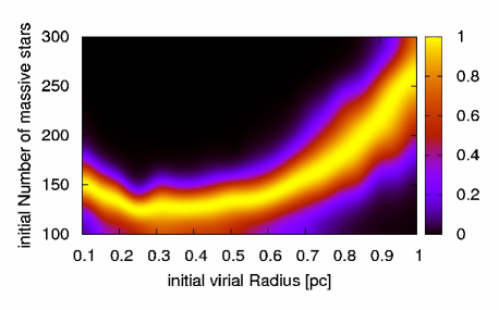
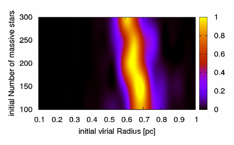
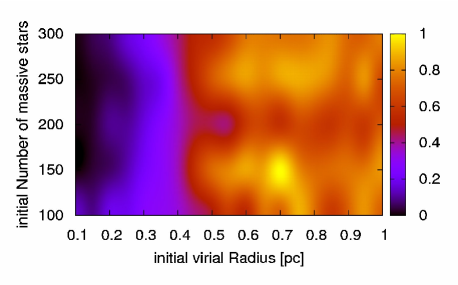
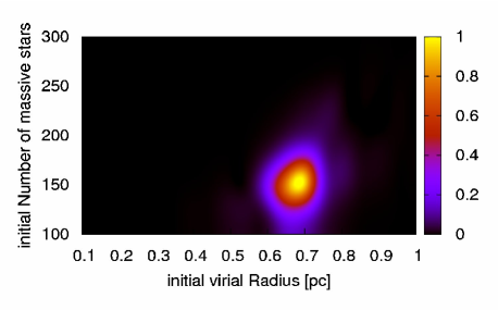
Figure 9: Quality of fit to observations for varying model parameters $R_{\mathrm{vir}}$ and $N_{\mathrm{MS}}$. Data from model IKW03S05 (isolated King model with $W_{0}=3$ and a Salpeter IMF with $m_{\mathrm{low}}=0.5\,{\rm M_{\odot}}$). Panels show the fit to the cluster mass (top left), cumulative mass profile (top right), IMF (bottom left) and product of all three fits (bottom right). A fitness parameter close or equal to unity indicates the best fit models and in the final panel an overall best fit model can be clearly identified.

The quality of the fit for model IKW03S05 is presented in Fig. 9, which shows how $f_{\mathrm{CMP}}$, $f_{\mathrm{M}}$, and $f_{\mathrm{IMF}}$ vary for the model parameters $R_{\mathrm{vir}}$ and $N_{\mathrm{MS}}$. The cluster mass is best fitted with $N_{\mathrm{MS}}\approx 150$ and almost independent of $R_{\mathrm{vir}}$. Only models with $R_{\mathrm{vir}}\geq 0.8$ require larger values of $N_{\mathrm{MS}}$. This can be explained as follows: models with small $R_{\mathrm{vir}}$ evolve faster dynamically and these models have gone through core collapse already at an age of $2.5\,\mathrm{Myr}$. As a result, the initial dependence of $N_{\mathrm{MS}}$ on $R_{\mathrm{vir}}$, which can still be seen for larger values of $R_{\mathrm{vir}}$, is lost.

The top right panel in Fig. 9 shows which models have the best fitting mass profiles. In this case, the best models are found within a narrow range of $R_{\mathrm{vir}}$-values with no dependence on $N_{\mathrm{MS}}$. Models with $R_{\mathrm{vir}}\leq 0.5\,\mathrm{pc}$ are, in comparison with the observations, too concentrated (see also Fig. 7) whereas $R_{\mathrm{vir}}>0.8\,\mathrm{pc}$ results in a too shallow mass profile.

The MF depends not as strongly on the model parameters (bottom left panel) though the general trend is, that the best fits are found for values of $R_{\mathrm{vir}}$ larger than $0.4\mathrm{pc}$. In the last panel, we show the combined fitness $f_{\mathrm{all}}$ which is defined as

$$f_{\mathrm{all}}=f_{\mathrm{CMP}}\cdot f_{\mathrm{M}}\cdot f_{\mathrm{IMF}}.$$ (8)

As a result, the best fitting model in the model series IKW03S05 can be clearly identified and it has an initial virial radius $R_{\mathrm{vir}}=0.70\,\mathrm{pc}$ and $N_{\mathrm{MS}}=150$. The number of stars with $m>10\,{\rm M_{\odot}}$ and inside $R<0.4\,\mathrm{pc}$ in this particular model is $208\pm 12$ (averaged over ten random realizations), compared to $234$ in the observed sample.

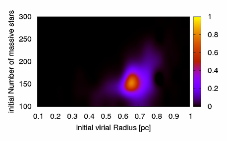
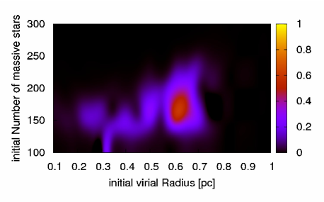
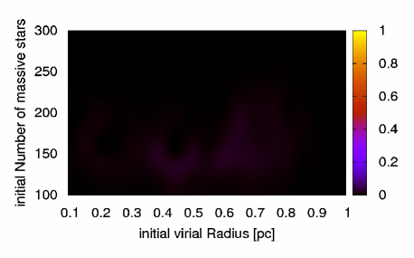
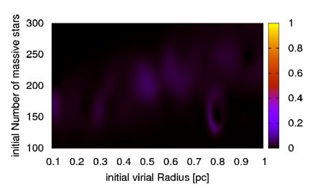
Figure 10: Quality of fit to observations for different models and varying model parameters $R_{\mathrm{vir}}$ and $N_{\mathrm{MS}}$. The combined fitness $f_{\mathrm{all}}$ is shown for models IKW03S10 (top left), IKW03S40 (top right), IKW03F05 (bottom left), and IKW07F10 (bottom right).

In Fig. 10 we compare $f_{\mathrm{all}}$ for a number of different model series. The two panels at the top show the results for the models IKW03S10 and IKW03S40. The only difference between these two models and also to model IKW03S05 shown in Fig. 9 is the lower mass limit of the IMF, which is $1.0$, $4.0$, and $0.5\,{\rm M_{\odot}}$, respectively. In each of the three models the best fit is in a similar regime of the parameter space, with $R_{\mathrm{vir}}=0.6-0.7\,\mathrm{pc}$ and $N_{\mathrm{MS}}\approx 150$. In all other model series that have an acceptable fit, the best fitting models also lie within a small area of the parameter space.

The two bottom panels show results from models starting initially with a flat IMF. These models produce no acceptable fit for any of our tested parameter combinations. The reason is that the slope of the IMF is always flattened by the dynamical evolution of the cluster (see also Fig. 8), so that models starting with the observed slope cannot produce a good fit. This result is independent of the initial concentration of the cluster and the lower cut-off mass of the IMF.

Table 2: Best fitting models.

Model	parameter		$f_{\mathrm{all}}$
	$R_{\mathrm{vir}}[\mathrm{pc}]$	$N_{\mathrm{MS}}$	$m>10\,{\rm M_{\odot}}$	$m>4\,{\rm M_{\odot}}$
IKW03F05	0.6	150	0.02	0.03
IKW03F10	0.35	150	0.06	0.03
IKW03S05	0.7	150	0.94	0.48
IKW03S10	0.65	150	0.78	0.52
IKW03S40	0.6	150	0.44	0.36
IKW05F05	0.45	150	0.04	0.07
IKW05F10	0.25	150	0.05	0.10
IKW05S10	0.8	200	0.65	0.44
IKW05S40	0.8	200	0.64	0.47
IKW07F05	0.75	250	0.05	0.04
IKW07F10	0.5	200	0.06	0.04
IKW07S10	1.0	200	0.55	0.36
IKW07S40	0.85	250	0.62	0.40

Columns are: 1) model name; 2) values of additional model parameter; 3) and 4) $f_{\mathrm{all}}$ comparing stars with $m>10\,{\rm M_{\odot}}$ and $m>4\,{\rm M_{\odot}}$

We have summarised the results in Tab. 2 where for each model series the best values for $R_{\mathrm{vir}}$ and $N_{\mathrm{MS}}$ are given together with the corresponding value of $f_{\mathrm{all}}$. We also repeated the whole analysis using all stars down to $4\,{\rm M_{\odot}}$ in the comparison. In both cases, models with the highest values of $f_{\mathrm{all}}$ all have a Salpeter IMF, though the comparison down to $4\,{\rm M_{\odot}}$ generally yields lower values for $f_{\mathrm{all}}$. This is not surprising as the uncertainties due to incompleteness and field contamination increase towards lower masses. It should also be noted, that the overall best fit model (IKW03S05) clearly stands out with $f_{\mathrm{all}}=0.94$, when the next best model has $f_{\mathrm{all}}=0.78$ (both models are different only in the lower mass limit).

The best fit models with a Salpeter IMF also have similar value of $R_{\mathrm{vir}}$ and $N_{\mathrm{MS}}$. We computed the average of these values weighted with $f_{\mathrm{all}}$ which results in $R_{\mathrm{vir}}=0.77\pm 0.12\,\mathrm{pc}$ and $N_{\mathrm{MS}}=183\pm 35$ for the comparison using stars with $m>10\,{\rm M_{\odot}}$. The initial mass of the cluster depends on the lower mass limit of the IMF. Our best model (and the favoured solution) has a lower mass limit $m_{\mathrm{lim}}$ of $0.5{\rm M_{\odot}}$, however models with a higher $m_{lim}$ also produce acceptable fits. Therefore, $m_{lim}$ is not well constrained by our models, which is to be expected since we only compare stars with $m>10\,{\rm M_{\odot}}$. In addition, observations are also limited by incompleteness and field contamination at lower masses ($m<4\,msun$ for the NACO data). Based on our results for stars with $m>10\,{\rm M_{\odot}}$, we get $M=\left(4.9\pm 0.8\right)\cdot 10^{4}\,{\rm M_{\odot}}$, $M=\left(3.6\pm 0.6\right)\cdot 10^{4}\,{\rm M_{\odot}}$, and $M=\left(1.9\pm 0.3\right)\cdot 10^{4}\,{\rm M_{\odot}}$ for lower mass limits of the IMF of $0.5$, $1$, $4\,{\rm M_{\odot}}$, respectively.

5 Discussion

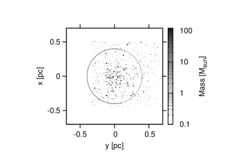
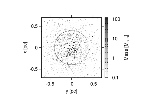
Figure 11: The observed cluster (left) and a snapshot of one of the best fitting models (IKW03S05, right) in comparison. The images are centred on the centre of density and the circles indicate a radius of $0.4\,\mathrm{pc}$. Gray-scale and point size represent stellar masses. In the right panel, stars have been removed randomly to mimic incompleteness.

A number of models in Tab. 2 can be considered best fit models, with the overall best fit being model IKW03S05 with $R_{\mathrm{vir}}=0.70$ and $N_{\mathrm{MS}}=150$. A snapshot of this model at $t=2.5\,\mathrm{Myr}$ is shown in Fig. 11. Stellar masses are indicated by the point size and gray-scale and the centre of density of the cluster is located at the origin. The dashed circle has a radius of $0.4\,\mathrm{pc}$. In the left panel, the NACO data is plotted for comparison in the same way as the simulation data in the right panel. In the latter, stars have been randomly removed to mimic incompleteness. The probability that a star is removed is given by a function fitted to the data shown in Fig. 2 and depends on mass and position of the star.

At $2.5\,\mathrm{Myr}$, the cluster in model IKW03S05 has a total mass of $\sim 1.8\cdot 10^{4}\,{\rm M_{\odot}}$ inside a radius of $0.4\,\mathrm{pc}$ and twice that mass inside the tidal radius of $1\,\mathrm{pc}$. Inside of $0.4\,\mathrm{pc}$, about $3\cdot 10^{3}\,{\rm M_{\odot}}$ of the total mass are in stars below $1\,{\rm M_{\odot}}$ ($9\cdot 10^{3}\,{\rm M_{\odot}}$ for $R<1\,\mathrm{pc}$). Espinoza et al. (2009) determined the cluster mass with $(2\pm 0.6)\cdot 10^{4}\,{\rm M_{\odot}}$ which is in agreement with out results. The models suggest that about half of the cluster’s mass is located in an annulus with $0.4<R<1\,\mathrm{pc}$. This result is in good agreement with the previous findings of Portegies Zwart et al. (2002).

Generally, only models with the Salpeter IMF produce acceptable fits and we therefore conclude that the IMF in the Arches cluster is consistent with having a normal Salpeter slope despite the extreme environment in which the cluster is formed. However, we cannot rule out a turn-over as suggested by (Stolte et al., 2005) as our results are not very sensitive to the lower mass limit of the IMF. Our best fitting models can have any lower mass limit in the the range of $0.5-4.0\,{\rm M_{\odot}}$ that we investigated, though the overall best fit has a lower limit of $0.5{\rm M_{\odot}}$.

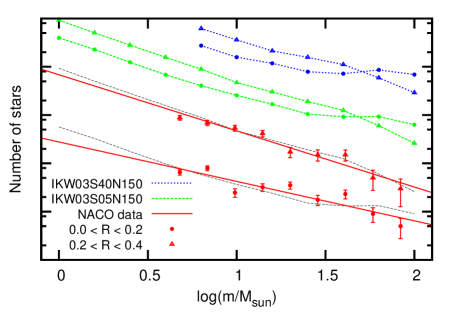
Figure 12: Comparing the observed MF in two radial bins. The full red lines are fitted power-law MF for the NACO data. The dashed green and the dotted blue lines connect the data points of the best fit models from the model series IKW03S05 and IKW03S40, respectively. The circles and triangles indicate data points from different radial bins and shifts of one or two dex have been applied to clarify the plot. For a better comparison, model IKW03S05 is also plotted without shifting (thin black line).

In Fig. 12, we compare the observed MF in two radial bins, namely $R<0.2\mathrm{pc}$ and $0.2<R<0.4\mathrm{pc}$ (the same as used by Stolte et al. (2005) and Espinoza et al. (2009)) with the observed model MF after $2.5\,\mathrm{Myr}$. A bin size of $\Delta\log(m/{\rm M_{\odot}})=0.2$ was used to obtain the individual star counts and the data from our best fit models was also averaged over the ten different realizations simulated. Two of the best fit models, IKW03S05 and IKW03S40, and the NACO are compared. For each data set, the circles and triangles mark the data points for the inner and outer radial bin, respectively. The full red lines show a fitted power-law MF for the NACO data. The dashed green and dotted blues lines connect the model data points.

The NACO data is fitted well by a single power-law and no break in the MF can be seen. We find slopes of $\Gamma=-0.8\pm 0.1$ and $\Gamma=-1.2\pm 0.1$ for the inner and outer radial bins, respectively. These slopes are slightly shallower than the slopes recently reported by Espinoza et al. (2009). The two model MFs for the outer radial bin can also be described by a single power-law with much the same slope. The model MFs in the inner radial bin are however noticeably flattened for massive stars ($m\mathrel{\mathchoice{\lower 3.6pt\vbox{\halign{$\mathsurround=0pt\displaystyle\hfil#\hfil$\cr>\crcr\sim\crcr}}}{\lower 3.6pt\vbox{\halign{$\mathsurround=0pt\textstyle\hfil#\hfil$\cr>\crcr\sim\crcr}}}{\lower 3.6pt\vbox{\halign{$\mathsurround=0pt\scriptstyle\hfil#\hfil$\cr>\crcr\sim\crcr}}}{\lower 3.6pt\vbox{\halign{$\mathsurround=0pt\scriptscriptstyle\hfil#\hfil$\cr>\crcr\sim\crcr}}}}10\,{\rm M_{\odot}}$). This behaviour can be best fitted by a broken power-law MF with a turning point at $m\approx 20{\rm M_{\odot}}$ and a shallow slope of $\Gamma=-0.3\pm 0.1$ at the high-mass end. In a related study, Portegies Zwart et al. (2007) also found a broken power-law MF, though in a radial bin similar to our outer bin (no data for an inner radial bin was shown Portegies Zwart et al. (2007)). The turning point in their favoured model was at $5-6{\rm M_{\odot}}$, however. They also noticed, that the break mass depended on the lower mass limit of the IMF which is not the case for our two best fit models IKW03S05 and IKW03S40. Both models have the same break mass but different lower mass limits ($0.5$ and $4{\rm M_{\odot}}$, respectively). The reason for these differences most likely is the different scaling used: Portegies Zwart et al. (2007) scale their models by the time scale $t_{\mathrm{cc}}$ for core collapse, while here we scale to physical units. Therefore, our models have evolved for different fractions of $t_{\mathrm{cc}}$ which results in different break masses (see also Fig. 2 in Portegies Zwart et al. (2007)).

In the Arches cluster, a possible turning point of the central MF could be indicated by the location of $5-6{\rm M_{\odot}}$-bump (Kim et al., 2006). The turn-over reported by Stolte et al. (2005) is also at this mass, however, models show an increase in the MF slope instead of the observed low-mass depletion. Generally, the observational data (both NACO and the data shown in Kim et al. (2006)) can be well described by a single power-law, whereas our models are better fitted by a broken power-law for the inner MF. Yet, the present-day MF from the observations and the model are still consistent with each other within the uncertainties of the observational data, as shown by the direct comparison between the NACO data and model IKW03S05 (thin black line in Fig. 12). Alternatively, a possible difference between the models and the observationally derived MFs could result from uncertainties in the stellar evolution models and in the incompleteness correction. The models, on the other hand, do not include the effects of stellar evolution and the tidal field. Another explanation could be primordial mass segregation (Chatterjee et al., 2009), which is not included in the present simulations.

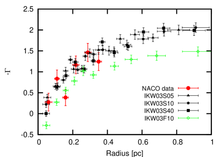
Figure 13: The slope $\Gamma$ of the observed MF as a function of radius. The NACO data is shown (red circles and error bars) in comparison to four best fit models (three with Salpeter IMF and one with a flat IMF).

In Fig. 13, we compare the slope $\Gamma$ of the observed MF that we derived from the NACO data and our best fit models. For each data set, we binned an equal number of stars into radial bins and determined $\Gamma$ as described before. Three of the models have a Salpeter IMF (black filled symbols) with different lower mass limits. The fourth model started with a flat IMF (green open symbol). In all four models and also the NACO data, the same flattening of the MF towards the centre can be seen. However, in comparison, the three models with a Salpeter IMF are in better agreement with the NACO data than the model with the flat IMF. The MF slopes of the latter are shifted by $\sim 0.4$ towards more positive $\Gamma$-values for $R<0.4\mathrm{pc}$ and even more at larger radii. The shift in the inner $0.4\mathrm{pc}$ is comparable to the initial difference between the Salpeter and the flat IMF. The flattening of the MF in the cluster core has been reported in all the previous observational studies, though with varying $\Gamma$-values determined for the slope. Our best fit models are in very good agreement, however, with the latest results from Espinoza et al. (2009) and also the results from Portegies Zwart et al. (2007). Our models predict a much steeper MF (steeper than Salpeter) for massive stars ($m>10{\rm M_{\odot}}$) at radii $R>0.4\mathrm{pc}$. It would therefore be very interesting to determine the MF slope at these larger radii. Unfortunately, it becomes very challenging to distinguish cluster and field stars beyond $0.4\mathrm{pc}$.

Dynamical Mass segregation combined with a radially limited selection of stars make the observed MF appear shallower than the global MF truly is. Stars with $m>10\,{\rm M_{\odot}}$ can be found in our models as far as $10\,\mathrm{pc}$ from the cluster centre. However, we find that in order to measure the correct slope of the MF, we only need the stars inside the tidal radius of $1\,\mathrm{pc}$.

No turn-over at the low mass end of the IMF can be seen. This means that the turn-over seen by Stolte et al. (2005) cannot be explained by mass segregation (unlike the flat IMF at the high-mass end). Deriving the IMF from our simulation data is not hampered by incompleteness, selection effects, and mass determination from observed luminosities. All these effects may bias the observed star counts to produce a turn-over, however, the turn-over appears at $\sim 6\,{\rm M_{\odot}}$ where the data is still 50% complete. So, either the IMF is indeed truncated or another effect has to be considered. One possible explanation is that tidal stripping preferably removes low-mass stars from the cluster. This effect is not included in our current simulations but will be tested in a follow-up paper. Alternatively, Espinoza et al. (2009) pointed out that local variations in extinction can account for (some of) the flattening of the observed MF. The same effect could leave lower-mass stars to be undetected preferentially. Then the completeness function, which only takes into account crowding and sensitivity effect, would not be sufficient to correct the low-mass end of the IMF.

Figure 14: The core radius evolution with time of model IKW03S05 with $R_{\mathrm{vir}}=0.7\,\mathrm{pc}$ and $N_{\mathrm{MS}}=150$. The black line with errorbars shows the average of ten random realizations of the same model (grey lines). Core collapse happens at $\sim 4\,\mathrm{Myr}$.

In Fig. 14 we show the core radius evolution with time for one of our best fit models (IKW03S05). At its current age of $2.5\,\mathrm{Myr}$ the cluster is more than halfway to core collapse which will occur at $\sim 4\,\mathrm{Myr}$ and a little more dynamically evolved than the favoured model in Portegies Zwart et al. (2007).

6 Summary

We have performed a large number of $N$-body simulations in order to find the best fitting model for the Arches cluster. The available observational data has been used to constrain the free parameters in our model. In a systematic analysis, we compared the total mass, the cumulative mass profile, and the present-day MF and defined fitness parameters for each of the three observables.

The main conclusion from our analysis is that the Arches cluster, despite of being born in an extreme environment, has formed with the slope of a standard Salpeter IMF. The lower mass-limit of the IMF is not from our models, but our models (as well as observations) show no indication that the IMF should be truncated well above $1{\rm M_{\odot}}$ or even $0.5{\rm M_{\odot}}$. Due to dynamical mass segregation, the slope of the observed MF is flattened inside a radius of $0.4\,\mathrm{pc}$. Outside this radius, our models predict a slope even steeper that Salpeter ($\Gamma\mathrel{\mathchoice{\lower 3.6pt\vbox{\halign{$\mathsurround=0pt\displaystyle\hfil#\hfil$\cr>\crcr\sim\crcr}}}{\lower 3.6pt\vbox{\halign{$\mathsurround=0pt\textstyle\hfil#\hfil$\cr>\crcr\sim\crcr}}}{\lower 3.6pt\vbox{\halign{$\mathsurround=0pt\scriptstyle\hfil#\hfil$\cr>\crcr\sim\crcr}}}{\lower 3.6pt\vbox{\halign{$\mathsurround=0pt\scriptscriptstyle\hfil#\hfil$\cr>\crcr\sim\crcr}}}}-2$). The radius of $0.4\mathrm{pc}$ was an imposed limit from the observational data used, and we estimate that a limiting radius of $\sim 1\,\mathrm{pc}$ would be required for the observed MF to match the underlying IMF.

We neglected the Galactic potential and also stellar evolution for the simulations in this paper. Both processes may have affected the evolution of the cluster only a little bit due to its young age of only $\sim 2.5\,\mathrm{Myr}$. If this is true our best fitting models suggest that the Arches cluster was born with an initial virial radius of $0.77\pm 0.12\,\mathrm{pc}$ and an initial total mass of about $(4.9\pm 0.8)\cdot 10^{4}\,{\rm M_{\odot}}$ assuming a lower mass limit of $0.5\,{\rm M_{\odot}}$ for the Salpeter IMF. The uncertainties in the lower mass limit give rise to additional uncertainties in determining the initial cluster mass. The King model concentration parameter of the best fitting models is $W_{0}=3$, however, more concentrated models with $W_{0}=5-7$ produced also reasonable fits so that this parameter is also not very well constrained.

The missing processes mentioned above will be included in a following paper to get a more realistic model of the Arches cluster. However this first step was needed in order to reduce the number of free parameters for these (computationally more expensive) simulations, which further constrain the dynamical evolution and tidal effects acting on the Arches cluster, and thereby the initial conditions of this nearby starburst, such as the cluster mass, the orbital motion and the IMF at the birth of the cluster.

Acknowledgements We thank the referee for helpful suggestions that improved this paper. SH and SPZ are grateful for the support from the NWO Computational Science STARE project #643.200.503 and NWO grant #639.073.803. AS acknowledges funding from the German Science Foundation (DFG) Emmy-Noether-Programme under grant STO 496-3/1.

References

- Bastian et al. (2010) Bastian N., Covey K. R., Meyer M. R., 2010, ArXiv e-prints
- Casertano & Hut (1985) Casertano S., Hut P., 1985, ApJ, 298, 80
- Chatterjee et al. (2009) Chatterjee S., Goswami S., Umbreit S., Glebbeek E., Rasio F. A., Hurley J., 2009, ArXiv e-prints
- Espinoza et al. (2009) Espinoza P., Selman F. J., Melnick J., 2009, A&A, 501, 563
- Figer et al. (1999) Figer D. F., Kim S. S., Morris M., Serabyn E., Rich R. M., McLean I. S., 1999, ApJ, 525, 750
- Figer et al. (1999) Figer D. F., McLean I. S., Morris M., 1999, ApJ, 514, 202
- Figer et al. (2002) Figer D. F., Najarro F., Gilmore D., Morris M., Kim S. S., Serabyn E., McLean I. S., Gilbert A. M., Graham J. R., Larkin J. E., Levenson N. A., Teplitz H. I., 2002, ApJ, 581, 258
- Gaburov et al. (2009) Gaburov E., Harfst S., Portegies Zwart S., 2009, New Astronomy, 14, 630
- Harayama et al. (2008) Harayama Y., Eisenhauer F., Martins F., 2008, ApJ, 675, 1319
- Heggie & Mathieu (1986) Heggie D. C., Mathieu R. D., 1986, in P. Hut & S. L. W. McMillan ed., The Use of Supercomputers in Stellar Dynamics Vol. 267 of Lecture Notes in Physics, Berlin Springer Verlag, Standardised Units and Time Scales. p. 233
- Kim et al. (2006) Kim S. S., Figer D. F., Kudritzki R. P., Najarro F., 2006, ApJ, 653, L113
- Kim et al. (2000) Kim S. S., Figer D. F., Lee H. M., Morris M., 2000, ApJ, 545, 301
- Kim et al. (1999) Kim S. S., Morris M., Lee H. M., 1999, ApJ, 525, 228
- King (1966) King I. R., 1966, AJ, 71, 64
- Kroupa (2002) Kroupa P., 2002, Science, 295, 82
- Lejeune & Schaerer (2001) Lejeune T., Schaerer D., 2001, A&A, 366, 538
- Martins et al. (2008) Martins F., Hillier D. J., Paumard T., Eisenhauer F., Ott T., Genzel R., 2008, A&A, 478, 219
- Najarro et al. (2004) Najarro F., Figer D. F., Hillier D. J., Kudritzki R. P., 2004, ApJ, 611, L105
- Portegies Zwart et al. (2007) Portegies Zwart S., Gaburov E., Chen H.-C., Gürkan M. A., 2007, MNRAS, 378, L29
- Portegies Zwart et al. (2010) Portegies Zwart S., McMillan S., Gieles M., 2010, ArXiv e-prints
- Portegies Zwart et al. (2002) Portegies Zwart S. F., Makino J., McMillan S. L. W., Hut P., 2002, ApJ, 565, 265
- Portegies Zwart et al. (2001) Portegies Zwart S. F., McMillan S. L. W., Hut P., Makino J., 2001, MNRAS, 321, 199
- Press et al. (1992) Press W. H., Teukolsky S. A., Vetterling W. T., Flannery B. P., 1992, Numerical recipes in FORTRAN. The art of scientific computing
- Salpeter (1955) Salpeter E. E., 1955, ApJ, 121, 161
- Stolte (2003) Stolte A., 2003, PhD thesis, Combined Faculties for the Natural Sciences and for Mathematics of the Ruperto-Carola University of Heidelberg, Germany for the degree of Doctor of Natural Sciences. III
- Stolte et al. (2005) Stolte A., Brandner W., Grebel E. K., Lenzen R., Lagrange A.-M., 2005, ApJ, 628, L113
- Stolte et al. (2008) Stolte A., Ghez A. M., Morris M., Lu J. R., Brandner W., Matthews K., 2008, ApJ, 675, 1278
- Stolte et al. (2002) Stolte A., Grebel E. K., Brandner W., Figer D. F., 2002, A&A, 394, 459