Quasielastic $\rho^{0}$$\rho^{0}$ $\rho^{0}$$\rho^{0}$  electroproduction on the proton at intermediate energy:
Role of scalar and pseudoscalar meson exchange

Abstract

We present a detailed analysis of $\rho^{0}$ electroproduction at intermediate energy for quasi-elastic knockout kinematics. The approach is based on an effective Lagrangian which generates exchanges of scalar, pseudoscalar, axial-vector and tensor mesons. The specific role of mesons with different values for $J^{PC}$ is analyzed. We show that the $\pi^{0}$ exchange amplitude and its interference terms with $\eta(\eta^{\prime})$ and $f_{1}$ exchanges dominate in the transverse part of the cross section $\sigma_{\scriptscriptstyle T}$. The main role plays the $\pi^{0}\to\rho^{0}$ M1 spin transition when coupling the virtual photons to the nucleon. In contrast, the longitudinal cross section $\sigma_{\scriptscriptstyle L}$ is generated by a series of scalar meson exchanges. To extract the dominant term more detailed information on the inner structure of scalar mesons is required. It turns out that recent data of the CLAS Collaboration on $\sigma_{\scriptscriptstyle L}$ and $\sigma_{\scriptscriptstyle T}$ can be described with reasonable accuracy if one proposes the quarkonium structure for the heavy scalar mesons ($M\gtrsim$ 1.3 GeV). On this basis the differential cross sections $d\sigma_{\scriptscriptstyle L}/dt$ and $d\sigma_{\scriptscriptstyle T}/dt$ are calculated and compared with the latest CLAS data.

I Introduction.

Recent data of the CLAS Collaboration clashad ; clasmor on electroproduction of the $\rho^{0}$ meson with separation of longitudinal $\sigma_{\scriptscriptstyle L}$ and transverse $\sigma_{\scriptscriptstyle T}$ parts of the cross section open up new possibilities in the study of the production mechanism. Experimental results on $\sigma_{\scriptscriptstyle L}$ and $\sigma_{\scriptscriptstyle T}$ obtained at relatively large photon virtualities of 1.5 $\lesssim Q^{2}\lesssim$ 4 GeV${}^{2}/c^{2}$ and at invariant energies $W\sim$ 2 – 3 GeV (i.e. above the resonance region) supplement the known data of the CLAS Collaboration on $\rho^{0}$ photoproduction clasbat since they contain new information on the $Q^{2}$–dependence of the cross sections. At large $Q^{2}$ some contributions to the cross section are small and in first approximation they can be excluded from the consideration. For example, at $Q^{2}\gtrsim$ 1.5 GeV²/c² contributions of intermediate baryon states ($N,\,N^{*}$, etc.) to the cross section are sufficiently suppressed in comparison to meson exchange contributions due to form factors encoding finite size effects in the $\gamma NN$, $\gamma NN^{*}$, $\rho NN$ and $\rho NN^{*}$ vertices.

An important feature of $\rho^{0}$ electroproduction is that different meson exchange mechanisms dominate in the longitudinal and transverse cross sections. This phenomenon allows to consider the contributions of these mesons separately, while the data on only the full cross section $\sigma=\sigma_{\scriptscriptstyle T}+\epsilon\,\sigma_{\scriptscriptstyle L}$ do not permit such a possibility. For example, data of the JLAB $F_{\pi}$ Collaboration on electroproduction of charged pions huber ; horn ; volmer allowed to deduce the charged pion form factor using the dominance of the pion $t$-pole contribution to the longitudinal part of the differential cross section $d\sigma_{\scriptscriptstyle L}/dt$. Note, that the transverse part $d\sigma_{\scriptscriptstyle T}/dt$ is dominated by the $\rho$–meson pole, and the JLab data huber ; horn ; volmer on $d\sigma_{\scriptscriptstyle T}/dt$ allow to perform an independent study of the $\rho$–meson exchange amplitude faess . It would be impossible to study both phenomena on the basis of the total cross section only.

These new possibilities for a detailed experimental study of the reaction $\gamma^{*}_{\scriptscriptstyle L,T}+p\to\rho^{0}+p$ in quasi-elastic kinematics can be used to gain insight into the structure of the meson cloud of the nucleon and into the quark origin of the electromagnetic properties of neutral mesons. Our present work is devoted to the theoretical study of this reaction in the context of these new possibilities that distinguish recent electroproduction experiments clashad ; clasmor from older ones cassel .

In the case of the $\gamma^{*}_{\scriptscriptstyle L,T}+p\to\rho^{0}+p$ reaction until recently there were only integral data (integral characteristics over the $t$ variable – the squared momentum transfer to the proton – see e.g. Ref. clashad ) which we have used as a basis for our consideration. Very recently data on the differential cross sections were also published by the CLAS Collaboration clasmor which allows for a further detailed test of the theory presented here.

The differential cross sections $d\sigma_{\scriptscriptstyle T}/dt$ and $d\sigma_{\scriptscriptstyle L}/dt$ are more informative: for small values of $t$ near the kinematical threshold $t-t_{min}\sim$ 0 (i.e. in the region of quasi-elastic meson knockout) the nearby $t$–channel pole dominates in each of these cross sections, which generates the forward peak of electroproduction in the absorption of either a longitudinal ($\gamma^{*}_{\scriptscriptstyle L}$) or transverse ($\gamma^{*}_{\scriptscriptstyle T}$) virtual photon. In the case of $\gamma^{*}_{\scriptscriptstyle L,T}+p\to\rho^{0}+p$ the pion $t$–pole contribution dominates in $\sigma_{\scriptscriptstyle T}$ and $t$ poles of the lightest scalar mesons dominate in $\sigma_{\scriptscriptstyle L}$. The dominant $t$ pole gives also a main contribution to the corresponding integrated cross section ($\sigma_{\scriptscriptstyle T}$ or $\sigma_{\scriptscriptstyle L}$), but contributions of heavy-meson exchanges (mesons with masses close to and above 1 GeV) are also important. Sometimes these corrections are quite significant since they interfere with the leading contributions of the light mesons.

Nevertheless, as the first step, the data on $\sigma_{\scriptscriptstyle L}$ and $\sigma_{\scriptscriptstyle T}$ clashad for the reaction $\gamma^{*}_{\scriptscriptstyle L,T}+p\to\rho^{0}+p$ can already be used to give an estimate for the dominant contributions. The additional (in comparison to electroproduction of charged mesons) selection rule connected with charge parity (C) conservation in the $\gamma\to\rho^{0}$ transition allows this procedure. Latter conservation law reduces the number of exchange diagrams to be considered. Here we also can use the models of vector meson dominance (VMD) and tensor meson dominance (TMD) renner for an estimate of the vertex constants in the $t$–channel pole terms oh using the underlying idea of charge universality.

In the reaction $\gamma^{*}_{\scriptscriptstyle L,T}+p\to\rho^{0}+p$ both the virtual photon and $\rho^{0}$ have the same (negative) charge parity, i.e. $J^{PC}=1^{--}$. Such a reaction cannot be considered as a true quasi-elastic knockout process, since here $\rho^{0}$– meson exchange is forbidden due to $C$–parity conservation. Therefore, such a “knockout” can proceed due to the conversion of a meson from the nucleon meson cloud into the final $\rho^{0}$ meson or due to the $\gamma\to\rho^{0}$ transition in a diffraction process. Since pion exchange ($J^{PC}=0^{-+}$) is allowed here the pion pole must dominate in the region of small $|t|$ (i.e. at small angles in quasi-elastic kinematics). However, the pion contribution only dominates in the transverse part of the cross section $\sigma_{\scriptscriptstyle T}$ due to the $M1$ spin transition $\pi^{0}\to\rho^{0}$. At the same time, the pion pole contribution to $\sigma_{\scriptscriptstyle L}$ is negligibly small even at values of $t\sim t_{min}$ – opposite to the situations of charged meson knockout processes. Pomeron exchange ($C=+$) is allowed but its contribution to $\sigma_{\scriptscriptstyle L}$ is too small in the region of invariant energies $W\sim$ 2 – 3 GeV considered when compared to the summation of the $t$-pole terms of other low-mass mesons.

For invariant energies $W$ slightly above the baryon resonance region and for high virtualities of the photon ($Q^{2}\sim$ 1.5 – 4 GeV²/c² in the JLAB experiments) it is sufficient to take into account the exchanges of neutral pseudoscalar mesons and additionally from the three nonets $J^{PC}=J^{++}$ with $J=$ 0,1,2 corresponding to the first orbital 1P excitation of the vector nonet (see Table I). Note, that we only consider mesons with positive charge parity (C=+) which give a contribution to the quasi–elastic knockout of $\rho^{0}$ supplemented either by spin flip ($M1$–transitions ${}^{1}S_{0}$ $\to$ ${}^{3}S_{1}$ without changing the spatial $P$-parity) or deexcitation of the orbital $1P$ state ($E1$–transitions ${}^{3}P_{J}$ $\to$ ${}^{3}S_{1}$ with change of the $P$-parity). In the first approximation one can neglect the highly excited meson nonets, because the corresponding orbital matrix elements of the transitions $2S\to 1S$, $2P\to 1S$, etc. must be suppressed in comparison to the $1S\to 1S$ and $1P\to 1S$ contributions.

Starting with energies of $W\sim$ 5 – 10 GeV and above the electroproduction cross section is suitably described in the framework of Regge phenomenology, which gives a reasonable description in a wider region of the variable $t$ than the $t$-pole approximation, – up to the region of hard collisions where partonic degrees of freedom become manifest. Then the most convenient description of the hadronic processes can be done in terms of generalized partonic distributions (see, e.g. clashad ; clasmor ; guidal ; kaskul ).

In a series of works laget1 ; laget2 ; laget3 ; cano the Regge phenomenology has been extended to the description of meson electro– and photoproduction cross sections at lower energies of about $W\sim$ 2 – 3 GeV. In this approach meson propagators in the exchanged diagrams are substituted by amplitudes of the corresponding Regge trajectories (R). The Pomeron trajectory (P) contribution is also included in the total sum. Here the coupling constants and form factors of low–energy hadron physics are used for the $\gamma R\rho$ and $RNN$ vertices. For the $\gamma R\rho$ vertex the dominance of vector mesons is used and a corresponding form factor is calculated in terms of the $q\bar{q}$ loop in the Landshoff-Donnachie approach landshoff . Since the vertex coupling constants (excluding the $\pi NN$ coupling) are only known with a low precision an additional free parameter laget3 ; cano is introduced into the amplitude which is normalized by data on $\rho^{0}$ photoproduction.

We should stress that in the energy region of $W\sim$ 2 – 3 GeV an equally good description of meson photo– and electroproduction cross sections can also be obtained on the basis of the usual pole approximation – also using phenomenological vertex form factors oh ; faess ; obukh ; neud2 . An advantage of the pole approximation is that the starting point is set up by effective Lagrangians. Therefore the momentum–spin structure of the meson vertices can be consistently taken into account which also defines the energy dependence of cross sections in the case of higher meson spins.

In Ref. clashad a reasonable description of the CLAS data on $\rho^{0}$ electroproduction has been obtained in the framework of a Regge model laget3 ; cano using the dominance of $\pi$, $\sigma$ and $f_{2}$ trajectories. The tensor $f_{2}$ meson was implemented as an isoscalar meson with positive $C$–parity and $J=$ 1 in accordance with the hypothesis that pomeron and $f_{2}$ trajectories are proportional. Also, an additional multiplier $\kappa_{f_{2}}$ was introduced to rescale the contribution of the $f_{2}$ trajectory relative to the one of the pomeron. The size of $\kappa_{f_{2}}$ was normalized to experimental data on $\rho^{0}$ photoproduction clasbat . As it turns out a significant enhancement of the $f_{2}$ trajectory contribution as compared to the pomeron trajectory ($\kappa_{f_{2}}=$ 9) is required. The $\sigma$ meson exchange has also been enhanced, because in laget3 a large value for the $\rho\sigma\gamma$ coupling was used ($g_{\rho\sigma\gamma}\approx$ 1, see details in cano ). Data on the $\rho\to\pi^{0}\pi^{0}\gamma$ decay width pdg ; snd can be explained using a much smaller value for the $g_{\rho\sigma\gamma}$ coupling snd .

All this has been analyzed in Ref. oh where the description of data on $\rho$ photoproduction obtained earlier by laget3 has been reconsidered. An alternative approach was proposed, where the amplitude of $\rho^{0}$ photoproduction was represented by the sum of the $t$–pole contributions from physical meson exchanges with coupling constants normalized to independent data ($s$- and $u$-pole contributions were taken into account as well). A good description of photoproduction data has been achieved in both approaches laget3 and oh . It seems that the $\sigma$ and $f_{2}$ mesons showing up in the Regge model laget3 are only effective degrees of freedom giving a useful parametrization of the total contribution by exchange of physical mesons listed in Table I.

In the present paper we also pursue an alternative description of the data on $\rho^{0}$ electroproduction similar to the approach of Ref. oh . We start with phenomenological Lagrangians to calculate the cross sections $\sigma_{\scriptscriptstyle L}$ and $\sigma_{\scriptscriptstyle T}$ in the $t$–pole approximation for the set of mesons displayed in Table I (see also Fig.1). In our calculation we use the coupling constants and form factors supported by and deduced from data and which mostly coincide with those already used in Ref. oh in the description of photoproduction data. The comparison of the theoretical results with latest data of the CLAS Collaboration clashad allows to determine the set of dominant meson exchanges corresponding to physical particles.

It will be found that in the description of the transverse cross section $\sigma_{\scriptscriptstyle T}$ the pion contribution and the summed contribution of pseudovector mesons ($f_{1},\,f_{1}^{\prime},\,a_{1}$) and other pseudoscalars ($\eta,\,\eta^{\prime}$) in interference with the pion piece play the major role. In addition, the summed contribution of mesons with positive $P$–parity ($f_{0},\,f_{2}$, $a_{0},\,a_{2}$) is practically not visible in $\sigma_{\scriptscriptstyle T}$ above such a background. In contrary, mesons with positive $P$–parity give a significant contribution to $\sigma_{\scriptscriptstyle L}$. However, if we use for all scalar $f_{0}$ mesons of Table I electromagnetic coupling constants $g_{\rho f_{0}\gamma}$ normalized to the known radiative decay widths of the $\sigma$ and $f_{0}(980)$ mesons, the contribution of all $f_{0}$,$a_{0}$,$f_{2}$ and $a_{2}$ mesons will be not sufficient to explain the data on $\sigma_{\scriptscriptstyle L}$.

In the final part of the paper we discuss different scenarios for overcoming these difficulties. It is shown that the problem can be solved using the set of known scalar mesons (i.e. without inclusion of possible exotic states) if the set of heavy scalars ($f_{0}(1370)$, $f_{0}(1500)$ and $f_{0}(1710)$ or at least two states from this group) are considered as ${}^{3}P_{0}$ states in the $\bar{q}q$ spectrum. According to the quark model such states should have relatively large radiative decay widths $\Gamma_{f_{0}\to\gamma\rho}\gtrsim$ 100 KeV kalash1 resulting in large coupling constants $\rho f_{0}\gamma$ with $g_{\rho f_{0}\gamma}>>g_{\rho\sigma\gamma}$ ($\bar{q}qg$ hybrid models with anomalous large widths kalash2 and models soy ; kissl with large values for the $\rho\sigma\gamma$ or $\sigma NN$ coupling also do not contradict data, but one can proceed without these assumptions). Furthermore, in addition to the included $\sigma$ meson exchange a non-correlated $2\pi$ exchange must also contribute to the cross section (recall that in Ref. oh it was shown that this mechanism plays an appreciable role in the $\rho^{0}$ photoproduction at low energy).

We present our final results on the integrated $\sigma_{\scriptscriptstyle L/T}$ and differential $d\sigma_{\scriptscriptstyle L/T}/dt$ cross sections where the previously indicated corrections for the coupling constants $g_{\rho f_{0}\gamma}$ of two heavy mesons $f_{0}(1370)$ and $f_{0}(1500)$ are included. The results for $\sigma_{\scriptscriptstyle L/T}$ are compared to the latest data of the CLAS Collaboration clashad ; clasmor . Theoretical curves are in agreement with data within experimental errors. The results for $d\sigma_{\scriptscriptstyle L/T}/dt$ appear to be in a good agreement with the new CLAS data clasmor as illustrated for several experimental bins in the range of 1.9 $<\,Q^{2}\,<$ 2.2 GeV${}^{2}/c^{2}$. A full analysis of all the experimental bins (more than 50 kinematical regions from $Q^{2}=$ 1.6 GeV${}^{2}/c^{2}$ and $x_{B}=$ 0.16 to $Q^{2}=$ 5.6 GeV${}^{2}/c^{2}$ and $x_{B}=$ 0.7) will be presented in a further paper in its own right.

II Framework

II.1 $t$–pole contributions due to exchange of mesons with positive $C$–parity

II.1.1 Scalar meson exchange ($S=f_{0}$, $a_{0}$)

We start with the effective Lagrangian

$${\cal L}_{\rho{\scriptscriptstyle S}\gamma}(x)=\frac{eg_{\rho S\gamma}}{4M_{\rho}}S(x)F_{\mu\nu}(x)\rho^{\mu\nu}(x),$$

$$F_{\mu\nu}=\partial_{\mu}A_{\nu}-\partial_{\nu}A_{\mu},\quad\rho_{\mu\nu}=\partial_{\mu}\rho_{\nu}-\partial_{\mu}\rho_{\nu},$$ (1)

$${\cal L}_{{\scriptscriptstyle SNN}}(x)=g_{{\scriptscriptstyle SNN}}S(x)\overline{N}(x)N(x)$$ (2)

which generates matrix elements due to the exchange of scalar mesons $S=f_{0},\,a_{0}$. The respective invariant amplitude is

$$T_{\scriptscriptstyle S}(s,s^{\prime},\lambda,\lambda_{\rho})=e\,\frac{g_{\rho{\scriptscriptstyle S}\gamma}}{M_{\rho}}g_{{\scriptscriptstyle SNN}}\frac{g_{\mu\nu}k^{\prime}\cdot q-k^{\prime}_{\nu}q_{\mu}}{k^{2}-M_{f_{0}}^{2}+i0}\\ \times{\epsilon_{\scriptscriptstyle V}^{(\lambda_{\rho})\mu}}^{*}\!(k^{\prime})\,\epsilon^{(\lambda)\nu}\!(q)\overline{u}(p^{\prime},s^{\prime})u(p,s),$$ (3)

where $\epsilon^{(\lambda)}_{\nu}(q)$ and $\epsilon_{{\scriptscriptstyle V}\,\mu}^{(\lambda_{\rho})}(k^{\prime})$ are the polarization vectors of photon and $\rho^{0}$ meson, respectively. They satisfy completeness relations in the subspace orthogonal to the 4–momentum:

$$\sum_{\lambda\!=\!0,\pm 1}(\!-\!1)^{\lambda}\epsilon^{(\lambda)}_{\mu}(q){\epsilon^{(\lambda)}_{\nu}}^{*}(q) = g_{\mu\nu}-\frac{q_{\mu}q_{\nu}}{q^{2}},$$

$$\sum_{\lambda_{\rho}\!=\!0,\pm 1}\epsilon_{{\scriptscriptstyle V}\,\mu}^{(\lambda_{\rho})}\!(k^{\prime}){\epsilon_{{\scriptscriptstyle V}\,\nu}^{(\lambda_{\rho})}}^{*}\!(k^{\prime}) = -\left[g_{\mu\nu}-\frac{k^{\prime}_{\mu}k^{\prime}_{\nu}}{M_{\rho}^{2}}\right].$$ (4)

Further, the invariant amplitude (3) is modified as usually by introducing vertex form factors

$$g_{\rho{\scriptscriptstyle S}\gamma}\to g_{\rho{\scriptscriptstyle S}\gamma}{\cal F}_{\rho{\scriptscriptstyle S}\gamma}(Q^{2},t),\quad g_{S{\scriptscriptstyle NN}}\to g_{S{\scriptscriptstyle NN}}{\cal F}_{S{\scriptscriptstyle NN}}(t),$$ (5)

where

$${\cal F}_{\rho{\scriptscriptstyle S}\gamma}(Q^{2},t)\equiv{\cal F}_{1}(Q^{2}){\cal F}_{2}(t)\,,\hskip 7.11317pt{\cal F}_{S{\scriptscriptstyle NN}}(t)\equiv{\cal F}_{3}(t)\,,$$ (6)

$t=k^{2}$ and $Q^{2}=-q^{2}$. The substitution (5) is equivalent to a nonlocal form of the interaction vertices efim ; ivanov ; fae , i.e. to the following modification of the local Lagrangians (1) and (2):

$${\cal L}_{\rho{\scriptscriptstyle S}\gamma}(x) \to {\cal L}^{NL}_{\rho{\scriptscriptstyle S}\gamma}(x)=\frac{eg_{\rho{\scriptscriptstyle S}\gamma}}{4M_{\rho}}\int\!d^{4}y\int\!d^{4}z\Phi_{1}(z^{2})\Phi_{2}(y^{2})$$

$$\times S(x+y)F_{\mu\nu}(x+z)\rho^{\mu\nu}(x)\,,$$

$${\cal L}_{{\scriptscriptstyle SNN}}(x) \to {\cal L}^{NL}_{{\scriptscriptstyle SNN}}(x)=g_{{\scriptscriptstyle SNN}}\int\!d^{4}y\,\Phi_{3}(y^{2})$$ (7)

$$\times S(x+y)\overline{N}(x)N(x),$$

where $\Phi_{i}(y^{2})$ are relativistic invariant vertex functions. In momentum space ${\cal F}_{i}(k^{2})=\int\Phi_{i}(y^{2})e^{ik\cdot y}d^{4}y$ defines the corresponding vertex form factor.

The factors $g_{\rho f_{0}\gamma}$ and ${\cal F}_{\rho f_{0}\gamma}(Q^{2},t)$ in the effective Lagrangian (1) should correspond to a specific physical process in the vertex. In particular, they should take into account the VMD transition $\gamma\to\rho^{0}$ with further diffractive scattering of the $\rho^{0}$ — in accordance with the diagram shown in Fig. 2a. An analogous process should contribute to the vertex $\rho\pi\gamma$ (see Fig. 2b) with the difference that here the spin $M1$ transition $\pi^{0}\to\rho^{0}$ is understood. As a result the dependence of the form factors ${\cal F}_{\rho f_{0}\gamma}(Q^{2},t)$ and ${\cal F}_{\rho\pi\gamma}(Q^{2},t)$ on the virtuality $Q^{2}$ of the photon is described by the propagator of the vector meson $\frac{1}{Q^{2}+M_{V}^{2}}$ in the first approximation. The dependence on $t$ involves the specific scale $\Lambda^{-1}$ corresponding to the size of the interaction volumes in the transitions $\rho^{0}+f_{0}\to\rho^{0}$ and $\omega+\pi\to\rho^{0}$ (see below).

The magnitudes of the $\rho S\gamma$ coupling constants can be estimated using the radiative decay width of the scalar meson $f_{0}$ with

$$\Gamma_{f_{0}\!\to\!\gamma\rho}=\alpha\,\frac{g_{\rho f_{0}\gamma}^{2}}{M_{\rho}^{2}}\left(\frac{M_{f_{0}}^{2}-M_{\rho}^{2}}{2M_{f_{0}}}\right)^{3},$$ (8)

while for the lightest scalar meson $f_{0}(600)\equiv\sigma$ the decay width for $\rho^{0}\to\gamma+\sigma$

$$\Gamma_{\rho\!\to\!\gamma\sigma}=\frac{\alpha}{3}\frac{g_{\rho\sigma\gamma}^{2}}{M_{\rho}^{2}}\left(\frac{M_{\rho}^{2}-M_{\sigma}^{2}}{2M_{\rho}}\right)^{3}$$ (9)

is used. In Eqs. (8) and (9) we use coupling constants $g_{\rho f_{0}\gamma}$ fixed on the mass–shell ($Q^{2}=$ 0, $t=M_{f_{0}}^{2}$). Therefore, the form factor (5) for the $\rho f_{0}\gamma$ vertex must be normalized at $Q^{2}=0$ as

$${\cal F}_{\rho{\scriptscriptstyle S}\gamma}(Q^{2}=0,t=M_{f_{0}}^{2})=1\,.$$ (10)

The $\sigma NN$ form factor is normalized according to

$${\cal F}_{\sigma{\scriptscriptstyle NN}}(t=0)=1,$$ (11)

since the constant $g_{\sigma{\scriptscriptstyle NN}}$ is defined from $NN$ scattering data at low energies in the limit $t\to$ 0.

According to the data of the SND Collaboration snd the width of $\rho^{0}$ decay into the channel with the lightest scalar meson $\sigma$ is sufficiently large: $\Gamma_{\rho\!\to\!\gamma\sigma}\approx$ 2.83 keV. Estimates of the decay width $\Gamma_{f_{0}\!\to\!\gamma\rho}$ are also known for heavier scalar mesons, e.g. for $f_{0}(980)$ ($\sim$ 3.4 keV) obtained in the framework of the molecular $K\bar{K}$ model $f_{0}(980)$ lyub ; kalash1 . In both cases we obtain quite similar predictions for the coupling constants:

$$\quad g_{\rho\sigma\gamma}/M_{\rho}=0.25/M_{\rho}=0.32\,GeV^{-1},$$

$$\quad g_{\rho f_{0}\gamma}/M_{\rho}\approx 0.21/M_{\rho}=0.27\,GeV^{-1}.$$ (12)

For the present purposes we use a unique value $g_{\rho\sigma\gamma}=$ 0.25 for all scalar mesons in the calculation of the total exchange contribution involving $f_{0}(600)$, $f_{0}(980)$, $f_{0}(1370),$ $f_{0}(1500)$ and $f_{0}(1710)$.

Presently no data are available to constrain the $f_{0}NN$ couplings except for the lightest scalar $\sigma=f_{0}(600)$. Here we take the value $g^{2}_{\sigma NN}/4\pi\simeq$ 4 $\div$ 8 commonly used in boson-exchange models of the $NN$ interaction. As a rough estimate for of the contribution of the higher mass $f_{0}$ exchanges we use the common value $g_{f_{0}NN}=$$g_{\sigma NN}=$ 10. We note that $\sigma_{T}$ is only weakly sensitive to even significant variation of the constants $g_{f_{0}NN}$. Only $\sigma_{L}$ allows to search for an averaged contribution of $f_{0}$ meson exchanges.

II.1.2 Pseudoscalar meson exchange ($S_{5}=\pi^{0}$, $\eta$, $\eta^{\prime}$)

The $t$–pole contribution due to pseudoscalar meson exchange is described as

$$T_{\pi^{0}}(s,s^{\prime},\lambda,\lambda_{\rho})=-\frac{eg_{\rho\pi\gamma}}{2m_{\scriptscriptstyle N}M_{\rho}}{\cal F}_{\rho\pi\gamma}(Q^{2},t)g_{\pi{\scriptscriptstyle NN}}{\cal F}_{\pi{\scriptscriptstyle NN}}(t)\\ \times\varepsilon^{\mu\nu\alpha\beta}\,\frac{\epsilon^{(\lambda)}_{\mu}\!(q)q_{\nu}\,{\epsilon_{{\scriptscriptstyle V}\,\alpha}^{(\lambda_{\rho})}}^{*}\!(k^{\prime}){k^{\prime}}_{\beta}}{M_{\pi}^{2}-k^{2}-i0}\,\overline{u}(p^{\prime},s^{\prime})\not\!k\gamma^{5}u(p,s),$$ (13)

where $g_{\rho\pi\gamma}$ and $g_{\pi{\scriptscriptstyle NN}}$ are the coupling constants related to the $\rho\pi\gamma$ and $\pi NN$ vertices. The vertex $\rho\pi\gamma$ is generated by an effective Lagrangian with a minimal number of derivatives:

$${\cal L}_{\rho\pi\gamma}(x)=\frac{eg_{\rho\pi\gamma}}{4M_{\rho}}\varepsilon^{\mu\nu\alpha\beta}F_{\mu\nu}(x)\vec{\rho}_{\alpha\beta}(x)\cdot\vec{\pi}(x)\,.$$ (14)

For the $\pi NN$ vertex we use a pseudovector coupling with $f_{\pi{\scriptscriptstyle NN}}=\frac{M_{\pi}}{2m_{\scriptscriptstyle N}}g_{\pi{\scriptscriptstyle NN}}$:

$${\cal L}_{\pi{\scriptscriptstyle NN}}(x)=\frac{g_{\pi{\scriptscriptstyle NN}}}{2m_{\scriptscriptstyle N}}\,\overline{N}(x)\gamma^{\mu}\gamma^{5}\vec{\tau}N(x)\cdot\partial_{\mu}\vec{\pi}(x)\,.$$ (15)

The coupling constant $g_{\rho\pi\gamma}$ is deduced from the $\rho^{0}\!\to\!\gamma+\pi^{0}$ decay width

$$\Gamma_{\rho\!\to\!\gamma\pi}=\frac{\alpha}{3}\,\frac{g_{\rho\pi\gamma}^{2}}{M_{\rho}^{2}}\left(\frac{M_{\rho}^{2}-M_{\pi}^{2}}{2M_{\rho}}\right)^{3}.$$ (16)

With the experimental value of $\Gamma_{\rho\!\to\!\gamma\pi}=$ 93$\pm$19 keV pdg we get

$$g_{\rho\pi\gamma}/M_{\rho}=0.658/M_{\rho}=0.848\,GeV^{-1}.$$ (17)

For the $\pi NN$ coupling constant we use the standard value of $g_{\pi{\scriptscriptstyle NN}}=$ 13.4.

For the $\eta$ and $\eta^{\prime}$ mesons we have correspondingly:

$$g_{\rho\eta\gamma}/M_{\rho}=1.230/M_{\rho}=1.585\,GeV^{-1},$$

$$g_{\rho\eta^{\prime}\gamma}/M_{\rho}=1.052/M_{\rho}=1.356\,GeV^{-1},$$ (18)

using $\Gamma_{\rho\!\to\!\gamma\eta}=$ 45 $\pm$ 3 keV and $\Gamma_{\eta^{\prime}\!\to\!\rho\gamma}=$ 60 $\pm$ 6 keV pdg . For the strong couplings $g_{\eta NN}$ and $g_{\eta^{\prime}NN}$ the SU(3) relation is used

$$g_{\eta_{\,8}{\scriptscriptstyle NN}}=\frac{3F-D}{\sqrt{3}(F+D)}g_{\pi{\scriptscriptstyle NN}}$$ (19)

for the mixing angle $\theta_{P}\approx\,-$10^∘ pdg defining the state $\eta^{\prime}=\eta_{1}\cos\theta_{P}+\eta_{8}\sin\theta_{P}$ (see e.g. Refs. kirch2 ; titov ). With $F/D=$ 0.575$\pm$0.016 hatsuda we get

$$g_{\eta{\scriptscriptstyle NN}}=4.38,\quad g_{\eta^{\prime}{\scriptscriptstyle NN}}=4.34,$$ (20)

where in addition we use the ratio $g_{\eta_{1}{\scriptscriptstyle NN}}:g_{\eta_{\,8}{\scriptscriptstyle NN}}=\sqrt{2}:1$ which follows from a quark-model evaluation of the non-strange components in $\eta_{1}$ and $\eta_{\,8}$.

II.1.3 Tensor meson exchange ($T=f_{2}$, $f_{2}^{\prime}$, $a_{2}$)

The Lagrangians for tensor meson interaction with nucleons and vector particles are constructed in the framework of tensor meson dominance (TMD) renner . We follow Ref. oh and only present necessary formulas for understanding the final results (see details in oh ).

The Lagrangian for a free tensor field $f_{\mu\nu}$ is described in the Fierz–Pauli framework and has a complicated form when external fields are included. However, the equations of motion are reduced to the usual Klein–Gordon equations for each independent component of the symmetric tensor field $f_{\alpha\beta}=f_{\beta\alpha}$:

$$(\partial_{\mu}^{2}-M^{2}_{\scriptscriptstyle T})f_{\alpha\beta}=0$$ (21)

with the additional constraints

$$\partial^{\,\alpha}\!f_{\alpha\beta}=0,\quad g^{\alpha\beta}f_{\alpha\beta}=0\,.$$ (22)

As result there are only 5 independent components of the tensor field with spin 2. The propagator of the tensor field has the form

$$G^{\alpha\beta;\alpha^{\prime}\beta^{\prime}}(k^{2}) = iP^{\alpha\beta;\alpha^{\prime}\beta^{\prime}}(k)\,\frac{1}{k^{2}-M_{\scriptscriptstyle T}^{2}},$$ (23)

$$P^{\alpha\beta;\alpha^{\prime}\beta^{\prime}}(k) = \frac{1}{2}\left({\overline{g}}^{\alpha\alpha^{\prime}}{\overline{g}}^{\beta\beta^{\prime}}+{\overline{g}}^{\beta\alpha^{\prime}}{\overline{g}}^{\alpha\beta^{\prime}}\right)-\frac{1}{3}{\overline{g}}^{\alpha\beta}{\overline{g}}^{\alpha^{\prime}\beta^{\prime}},$$

$${\overline{g}}^{\alpha\beta} = -g^{\alpha\beta}+\frac{k^{\alpha}k^{\beta}}{M_{\scriptscriptstyle T}^{2}}\,.$$

The electromagnetic vertex $\gamma^{*}+f_{2}\to\rho^{0}$ depends on 4 Lorentz indices of the tensor and vector fields $f_{\alpha\beta},\,A_{\mu},\,\rho_{\nu}$ and is described as a sum of two independent Lorentz-covariant terms with corresponding coupling constants $f_{\rho f_{2}\gamma}$ and $g_{\rho f_{2}\gamma}$ renner ; oh :

$$\Gamma^{\alpha\beta;\mu\nu}(k^{\prime},q)=\frac{ef_{\rho f_{2}\gamma}}{M_{f_{2}}^{2}}\biggl{[}-g^{\mu\nu}q\cdot k^{\prime}+{k^{\prime}}^{\nu}q^{\mu}\biggr{]}$$ (24)

$$\times (q+k^{\prime})^{\alpha}(q+k^{\prime})^{\beta}+eg_{\rho f_{2}\gamma}\biggl{[}g^{\mu\nu}(q+k^{\prime})^{\alpha}(q+k^{\prime})^{\beta}$$

$$- g^{\mu\alpha}{k^{\prime}}^{\nu}(q+k^{\prime})^{\beta}-g^{\mu\beta}{k^{\prime}}^{\nu}(q+k^{\prime})^{\alpha}-g^{\nu\alpha}q^{\mu}(q+k^{\prime})^{\beta}$$

$$- g^{\nu\beta}q^{\mu}(q+k^{\prime})^{\alpha}+2q\cdot k^{\prime}(g^{\nu\alpha}g^{\mu\beta}+g^{\nu\beta}g^{\mu\alpha})\biggr{]}\,.$$

The strong coupling $f_{2}NN$ also includes two independent Lorentz covariant terms:

$$\Gamma^{\alpha\beta}(p,p^{\prime}) = \frac{G_{f_{2}NN}}{m_{\scriptscriptstyle N}}\left[(p+p^{\prime})^{\alpha}\gamma^{\beta}+(p+p^{\prime})^{\beta}\gamma^{\alpha}\right]$$ (25)

$$+ \frac{F_{f_{2}NN}}{m_{\scriptscriptstyle N}^{2}}(p+p^{\prime})^{\alpha}(p+p^{\prime})^{\beta}\,.$$

The magnitudes of the coupling constants $f_{\rho f_{2}\gamma}$, $g_{\rho f_{2}\gamma}$, $F_{f_{2}NN}$ and $G_{f_{2}NN}$ can be estimated in the framework of VMD and TMD models (see details in  renner ; oh ). In particular, the couplings are expressed in terms of two universal constants $g_{\scriptscriptstyle V}$ and $g_{\scriptscriptstyle T}$:

$$eg_{\rho f_{2}\gamma} = e\frac{g_{f_{2}{\scriptscriptstyle VV}}}{f_{\rho}M_{f_{2}}}=e\frac{g_{\scriptscriptstyle T}}{g_{\scriptscriptstyle V}M_{f_{2}}},\quad G_{f_{2}{\scriptscriptstyle NN}}=\frac{m_{\scriptscriptstyle N}}{2M_{f_{2}}}g_{\scriptscriptstyle T},$$

$$f_{\rho f_{2}\gamma} = F_{f_{2}{\scriptscriptstyle NN}}=0,$$ (26)

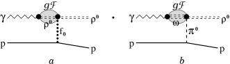
Figure 1: $t$–pole amplitude generated by meson exchanges.

Figure 2: Microscopic mechanism for the $\rho f_{0}\gamma$ and $\rho\pi\gamma$ couplings.

Figure 3: Tensor meson contribution to the vector meson electroproduction in VMD and TMD models.

Figure 4: Amplitudes of tensor meson decay into $\pi\pi$ in VMD and TMD models.

where $f_{\rho}=g_{\rho\pi\pi}=g_{\scriptscriptstyle V}$, $g_{f_{2}{\scriptscriptstyle VV}}=g_{f_{2}\pi\pi}=g_{\scriptscriptstyle T}$. The diagrams in Figs. 4 and 4 illustrate these conditions.

Tensor meson exchange contributions are described by the amplitude

$$T_{f_{2}}(s,s^{\prime},\lambda,\lambda_{\rho}) = \frac{2eg_{\rho f_{2}\gamma}G_{f_{2}NN}}{m_{\scriptscriptstyle N}(t-M_{f_{2}}^{2})}\,{\cal F}_{\rho f_{2}\gamma}(q^{2},t){\cal F}_{f_{2}NN}(t)$$ (27)

$$\times \overline{u}(p^{\prime},s^{\prime})\Gamma_{f_{2}}u(p,s)\,,$$

where

$$\Gamma_{f_{2}} = ({\epsilon_{{\scriptscriptstyle V}}^{(\lambda_{\rho})}}^{*}\epsilon^{(\lambda)})\biggl{[}\left((p\!+\!p^{\prime})(q\!+\!k^{\prime})\right)(\not\!q\!+\!\not\!k^{\prime})$$

$$+ \frac{2m_{\scriptscriptstyle N}}{3}\biggl{(}(q\!+\!k^{\prime})^{2}-\frac{1}{M_{f_{2}}^{2}}(k\cdot(q\!+\!k^{\prime}))^{2}\biggr{)}\biggr{]}$$

$$+ 2qk^{\prime}\biggl{[}((p\!+\!p^{\prime}){\epsilon_{{\scriptscriptstyle V}}^{(\lambda_{\rho})}}^{*})\not\!\epsilon^{(\lambda)}+((p\!+\!p^{\prime})\epsilon^{(\lambda)})\not{\epsilon_{{\scriptscriptstyle V}}^{(\lambda_{\rho})}}^{*}$$

$$+ \frac{4m_{\scriptscriptstyle N}}{3}\biggl{(}({\epsilon_{{\scriptscriptstyle V}}^{(\lambda_{\rho})}}^{*}\epsilon^{(\lambda)})-\frac{1}{M_{f_{2}}^{2}}({\epsilon_{{\scriptscriptstyle V}}^{(\lambda_{\rho})}}^{*}k)(\epsilon^{(\lambda)}k)\biggr{)}\biggr{]}\,.$$

Here we introduced the vertex form factors ${\cal F}_{\rho f_{2}\gamma}(q^{2},t)$ and ${\cal F}_{f_{2}NN}(t)$. These modify the constants $g_{\rho f_{2}\gamma}$ and $G_{f_{2}NN}$ in analogy with Eqs. (5)– (7) as:

$$g_{\rho f_{2}\gamma} \to g_{\rho f_{2}\gamma}{\cal F}_{\rho f_{2}\gamma}(Q^{2},t)\,,$$

$$G_{f_{2}NN} \to G_{f_{2}NN}{\cal F}_{f_{2}NN}(t)\,.$$ (29)

The values of these constants (see Fig. 4), $g_{\scriptscriptstyle V}$= 5.33 and $g_{\scriptscriptstyle T}$= 5.76, have been obtained using the decay data, $\Gamma_{\rho\to\pi\pi}=$ 150 MeV and $\Gamma_{f_{2}\to\pi\pi}=$ 156.5 MeV pdg , and the expressions:

$$\Gamma_{\rho^{0}\to\pi\pi} = \frac{g_{\scriptscriptstyle V}^{2}}{4\pi}\,\frac{M_{\rho}}{12}\left(1-\frac{4M_{\pi}^{2}}{M_{\rho}^{2}}\right)^{3/2},$$

$$\Gamma_{f_{2}\to\pi\pi} = \frac{g_{\scriptscriptstyle T}^{2}}{4\pi}\,\frac{M_{f}}{20}\left(1-\frac{4M_{\pi}^{2}}{M_{f}^{2}}\right)^{5/2}\,.$$ (30)

Here we suppose ideal mixing between $f_{2}(1270)$ and $f_{2}^{\prime}(1525)$. This means that the coupling of $f_{2}^{\prime}(1525)$ to the $\pi\pi$ channel is suppressed by the Okubo, Zweig and Iizuka rule as observed in experiment pdg . Therefore, in the first approximation one can neglect the contribution of $f_{2}^{\prime}(1525)$ in the electroproduction of $\rho^{0}$.

II.1.4 Axial-vector meson exchange ($V_{5}=f_{1}$, $f_{1}^{\prime}$, $a_{1}$)

Considering the $J^{PC}=1^{++}$ particle $V_{5}$ as a quark-antiquark ${}^{3}P_{1}$ bound state one can write the coupling $1^{++}\to\gamma^{*}(q)V(k^{\prime})$ in a form analogous to the ${}^{3}P_{1}\to\gamma^{*}\gamma^{*}$ coupling calculated in the quark model (see, e.g. cahn ):

$${\cal M}(1^{++}\to\gamma^{*}V)={\epsilon_{{\scriptscriptstyle V}\nu}^{(\lambda_{\rho})}}^{*}\!\Gamma^{\alpha,\mu\nu}_{{\scriptscriptstyle V}_{5}}\,\epsilon_{\mu}^{(\lambda)}\epsilon_{{\scriptscriptstyle V}_{5}\alpha},$$

$$\Gamma^{\alpha,\mu\nu}_{{\scriptscriptstyle V}_{5}}=eg_{\rho{\scriptscriptstyle V}_{5}\gamma}\varepsilon^{\mu\nu\alpha\beta}\frac{{k^{\prime}}^{2}q_{\beta}-q^{2}k^{\prime}_{\beta}}{M^{2}},\quad q^{\mu}\epsilon^{(\lambda)}_{\mu}(q)=0$$ (31)

($V=\rho^{0}$ and $\epsilon_{{\scriptscriptstyle V}_{5}\alpha}$ is the polarization vector of $V_{5}$). Here it is implied that the radial derivative $R_{q\bar{q}}^{\prime}(0)$ of the $q\bar{q}$ wave function is included to the constant $g_{\rho{\scriptscriptstyle V}_{5}\gamma}$ and the coupling can be further modified by a form factor.

Starting with this analogy we introduce the interaction Lagrangian

$${\cal L}_{\rho{\scriptscriptstyle V}_{5}\gamma}(x)=e\frac{g_{\rho{\scriptscriptstyle V}_{5}\gamma}}{M_{\rho}^{2}}\varepsilon^{\mu\nu\alpha\beta}V_{5\,\alpha}(\partial_{\beta}A_{\mu}\square\rho_{\nu}\\ -\partial_{\beta}\rho_{\nu}(g_{\mu\mu^{\prime}}\square-\partial_{\mu}\partial_{\mu^{\prime}})A^{\mu^{\prime}})$$ (32)

$${\cal L}_{{\scriptscriptstyle V}_{5}{\scriptscriptstyle NN}}(x)=g_{{\scriptscriptstyle V}_{5}{\scriptscriptstyle NN}}\,\overline{N}(x)\gamma^{\alpha}\gamma^{5}N(x)V_{5\,\alpha}(x),$$ (33)

and write down the $t$–pole axial-vector meson contribution to the electroproduction amplitude modified by form factors:

$$T_{V_{5}}(s,s^{\prime},\lambda,\lambda_{\rho})=-eg_{\rho{\scriptscriptstyle V}_{5}\gamma}g_{{\scriptscriptstyle V}_{5}{\scriptscriptstyle NN}}{\cal F}_{\rho{\scriptscriptstyle V}_{5}\gamma}(q^{2},t){\cal F}_{{\scriptscriptstyle V}_{5}{\scriptscriptstyle NN}}(t)$$ (34)

$$\times \varepsilon^{\mu\nu\alpha\beta}\left(q_{\nu}-\frac{q^{2}}{M_{\rho}^{2}}k_{\nu}^{\prime}\right)\epsilon^{(\lambda)}_{\mu}\!(q){\epsilon_{{\scriptscriptstyle V}\,\alpha}^{(\lambda_{\rho})}}^{*}\!(k^{\prime})$$

$$\times \frac{g_{\beta\beta^{\prime}}-k_{\beta}k_{\beta^{\prime}}/M_{f}^{2}}{k^{2}-M_{f}^{2}}\overline{u}(p^{\prime},s^{\prime})\gamma^{\beta^{\prime}}\gamma^{5}u(p,s)\,.$$

On this basis the radiative decay $f_{1}\to\gamma\rho$ width is calculated as:

$$\Gamma_{f_{1}\!\to\!\gamma\rho}=\frac{\alpha}{3}\,\frac{g_{\rho f_{1}\gamma}^{2}}{M_{\rho}^{2}}\left(1+\frac{M_{\rho}^{2}}{M_{f_{1}}^{2}}\right)\left(\frac{M_{f_{1}}^{2}-M_{\rho}^{2}}{2M_{f_{1}}}\right)^{3}.$$ (35)

Using the experimental value $\Gamma_{f_{1}\!\to\!\gamma\rho}=1.34\pm 0.32$ MeV pdg we get:

$$g_{\rho f_{1}\gamma}/M_{\rho}=1.901/M_{\rho}=2.45\ {\rm GeV}^{-1},$$

$$g_{\rho f_{1}^{\prime}\gamma}/M_{\rho}=0.582/M_{\rho}=0.748\ {\rm GeV}^{-1}\,.$$ (36)

To get $g_{\rho f_{1}^{\prime}\gamma}$ we have used quark counting kalash3 for the matrix element of the charge operator

$$e_{q}=\sum_{i}\left(\frac{1}{2}\lambda^{(i)}_{3}\!+\!\frac{1}{2\sqrt{3}}\lambda^{(i)}_{8}\right)$$ (37)

in neutral meson–meson transitions of opposite $C$-parity (in our case we deal with the transitions $f_{1}\to\rho^{0}$, $f_{1}^{\prime}\to\rho^{0}$ and $a_{1}\to\rho^{0}$). The dependence of the matrix element on the isospin part of the meson ($f_{n}$ or $a_{n}$) wave function is described by the simple relations kalash3 :

$$\langle f_{n}(I\!=\!0)|e_{q}|a_{n}(I\!=\!1)\rangle=1,$$

$$\langle f_{n}(I\!=\!1)|e_{q}|f_{n}(I\!=\!1)\rangle=\frac{1}{3},$$

$$\langle a_{n}(I\!=\!0)|e_{q}|a_{n}(I\!=\!0)\rangle=\frac{1}{3}.$$ (38)

The final results for the $f_{1}(1285)$ and $f_{1}^{\prime}(1410)$ mesons

$$\langle\rho^{0}|e_{q}|f_{1}^{\prime}\rangle/\langle\rho^{0}|e_{q}|f_{1}\rangle=\sin\epsilon\,/\cos\epsilon\,,\\ g_{\rho f_{1}^{\prime}\gamma}=g_{\rho f_{1}\gamma}\tan\epsilon\qquad$$ (39)

only depend on the mixing angle $\epsilon\approx$ 17^∘ bolt relating nonstrange and strange components in the initial meson (the final meson is the isovector $\rho^{0}=(\bar{u}u-\bar{d}d)/\sqrt{2}$) with

$$f_{1}(1285) = \cos\epsilon\frac{\bar{u}u+\bar{d}d}{\sqrt{2}}-\sin\epsilon\,\bar{s}s,$$

$$f_{1}(1410) = \sin\epsilon\frac{\bar{u}u+\bar{d}d}{\sqrt{2}}+\cos\epsilon\,\bar{s}s.$$ (40)

For the axial-vector isovector meson $a_{1}(1260)$ the corresponding coupling in the electromagnetic transition $a_{1}+\gamma\to\rho^{0}$ can be expressed through the constant $g_{\rho f_{1}\gamma}$ also using relations (38): $g_{\rho a_{1}\gamma}=\frac{1}{3}g_{\rho f_{1}\gamma}$. This is also fulfilled for any type of $f_{n}(a_{n})$ meson considered here and we accept

$$g_{\rho a_{n}\gamma}=\frac{1}{3}g_{\rho f_{n}\gamma},\quad n=J=0,\,1,\,2.$$ (41)

In Ref. kirch1 an estimate for the couplings of the $f_{1}(1285)$ and $f_{1}^{\prime}(1410)$ mesons to nucleons was obtained using the hypothesis of partial conservation of the axial-vector current, i.e. in analogy to the VMD model, which in this case is extended to neutral axial-vector mesons. According to Ref. kirch1 $|g_{f_{1}{\scriptscriptstyle NN}}|=$ 1.46 and $|g_{f_{1}^{\prime}{\scriptscriptstyle NN}}|=$ 10.5. If the neutral axial-vector current is only connected to the strange component in the nucleon kirch1 ; elis then, following (40), it follows that these couplings have different signs and we use the values

$$g_{f_{1}{\scriptscriptstyle NN}}=-1.46,\quad g_{f_{1}^{\prime}{\scriptscriptstyle NN}}=10.5\,.$$ (42)

II.2 Form factors

Finally in this section we make a few comments concerning the vertex form factors ${\cal F}_{\rho{\scriptscriptstyle M}\gamma}$ and ${\cal F}_{\scriptscriptstyle MNN}$ showing up in expression for ${\cal N}_{\scriptscriptstyle M}$ (see Table III). In the calculations we use a common monopole form factor describing the dependence on the virtuality of the (absorbed) particle in the case that the other two are on the mass shell:

$${\cal F}_{\gamma M\rho^{0}}(Q^{2},t\!=\!M_{\scriptscriptstyle M}^{2})=\frac{\Lambda_{q}^{2}}{\Lambda_{q}^{2}+Q^{2}},\\ {\cal F}_{{\scriptscriptstyle MNN}}(t)=\frac{\Lambda_{t}^{2}}{\Lambda_{t}^{2}-t},\quad\Lambda_{t}=\Lambda_{q}=M_{\rho}.$$ (43)

For the upper vertex in the diagrams of Fig.4 this form factor is the propagator of the virtual vector meson in the VMD. The same is also true for the form factors in the upper vertex of the analogous diagram of Fig.4. In the interpretation of the form factor as the Fourier transform of the function $\Phi(y^{2})$ (describing a nonlocal interaction in (7)) the expression of Eq. (43) takes only into account the characteristic scale $\sim\frac{1}{\Lambda}\approx\frac{1}{M_{\rho}}$ of the charge distribution of (any sort) in the hadron (but this is quite sufficient for our purposes). This procedure is also based on a similar description for quasi–elastic knockout of pions on the nucleon neud2 ; faess with similar kinematics. The corresponding magnitude of $\Lambda_{t}$ is correlated with data on $\pi^{+}$ electroproduction huber ; horn ; volmer .

If a vertex in the diagram contains two off–shell particles (as is the case for the upper vertex in the diagrams of Figs. 4 and 4), then a form factor should depend on both virtualities: $t-M_{M}^{2}$ and $Q^{2}$. In the case of pion exchange in the quasi–elastic knockout ($t\approx$ 0) the virtuality on t is negligible $M_{\pi}^{2}-t\approx$ 0 and the $t$–dependence in the $\gamma\pi\rho$ vertex can be neglected. However, in case of heavy meson exchange $M=f_{0}(a_{0}),f_{1}(a_{1}),f_{2}(a_{2})$ we cannot neglect the dependence on the virtuality $t-M_{\scriptscriptstyle M}^{2}$ for typical values of the momentum transfer squared $t\approx t_{min}$ in quasi–elastic knockout. Therefore we use for the $\gamma M\rho$ form factor a more complicated parametrization:

$${\cal F}_{\gamma M\rho^{0}}(Q^{2},t) = \frac{\Lambda_{q}^{2}}{\Lambda_{q}^{2}+Q^{2}}\,\frac{\Lambda_{0}^{2}}{\Lambda_{0}^{2}+M_{\scriptscriptstyle M}^{2}-t},$$

$$M_{\scriptscriptstyle M} = M_{f_{0}(a_{0})},\,M_{f_{1}(a_{1})}.$$ (44)

Here the second factor is normalized to 1 for $t=M_{\scriptscriptstyle M}^{2}$ — in correspondence with the normalization of the coupling $\gamma M\rho^{0}$ for the observable decay widths chosen in Eqs. (8) - (12), (30) and (35) - (36). We use in the form factor (44) the same value for the cutoff $\Lambda^{2}_{0}=$ 1.2 GeV${}^{2}/c^{2}$ as in Ref. faess . There we showed that such a parametrization is successful to describe data on the electroproduction of pions huber ; horn ; volmer in the framework of an analogous $t$-pole mechanism with the off–shell $\gamma\rho\pi$ coupling.

In the literature the $t$–dependence of the form factor (44) is usually represented in the form $\frac{\tilde{\Lambda}_{0}^{2}-M_{M}^{2}}{\tilde{\Lambda}_{0}^{2}-t}$ with approximately the same value for $\tilde{\Lambda}_{0}\approx$ 1.2–1.5 GeV$/c$. For a relatively small value of the meson mass $M_{\scriptscriptstyle M}\lesssim$ 1 GeV in expression (44) both parametrizations lead to approximately the same results in the considered region $t\sim$ 0. For more massive mesons $M_{\scriptscriptstyle M}\gtrsim$ 1.3–1.5 GeV the value of $\tilde{\Lambda}_{0}$ will depend on the meson mass. To avoid the introduction of new free parameters we use the parametrization (44) for all the $f_{0}(a_{0})$ and $f_{1}(a_{1})$ mesons. Only in the case of the $f_{2}$ meson we keep the standard parametrization (for the value of $\Lambda_{f_{2}}=$ 1.4 GeV$/c$),

$${\cal F}_{\gamma f_{2}\rho^{0}}(Q^{2},t) = \frac{\Lambda_{q}^{2}}{\Lambda_{q}^{2}+Q^{2}}\,\frac{\Lambda_{f_{2}}^{2}-M_{f_{2}}^{2}}{\Lambda_{f_{2}}^{2}-t},$$

$${\cal F}_{f_{2}{\scriptscriptstyle NN}}(t) = \frac{\Lambda_{f_{2}}^{2}-M_{f_{2}}^{2}}{\Lambda_{f_{2}}^{2}-t}\,,$$ (45)

which was already used by other authors (see e.g. Ref. oh and references therein).

III Electroproduction cross section: transverse and longitudinal parts

Recent experiments of the CLAS clashad ; clasmor ; clasphi and $F_{\pi}$ huber ; horn ; volmer Collaborations at JLAB on meson electroproduction in the quasi–elastic region allow in principle to separate individual meson exchange contributions. Therefore the corresponding electromagnetic and strong vertex form factors can be measured directly. In particular, in the CLAS experiments clashad ; clasmor ; huber ; horn ; volmer the differential cross section of meson electroproduction is separated in longitudinal ($L$), transverse ($T$) and mixed ($TT$, $LT$) parts as

$$\frac{d^{4}\sigma}{dW^{2}dQ^{2}dtd\varphi_{\scriptscriptstyle M^{\prime}}} = \Gamma\left\{\varepsilon\frac{d\sigma_{\scriptscriptstyle L}}{dt}+\frac{d\sigma_{\scriptscriptstyle T}}{dt}+\varepsilon\frac{d\sigma_{\scriptscriptstyle TT}}{dt}\cos 2\varphi_{\scriptscriptstyle M^{\prime}}\right.$$ (46)

$$+ \left.\sqrt{2\varepsilon(1+\varepsilon)}\frac{d\sigma_{\scriptscriptstyle LT}}{dt}\cos\varphi_{\scriptscriptstyle M^{\prime}}\right\}$$

by varying $\varepsilon$ and $\phi_{\scriptscriptstyle M^{\prime}}$ (via the Rosenbluth separation).

In Eq. (46) $W^{2}$ is the square of the invariant mass with $W^{2}=s=(q+p)^{2}=(k^{\prime}+p^{\prime})^{2}$; $p$ and $p^{\prime}$ are the 4-momenta of the target and recoil nucleon respectively, $k^{\prime}$ is the 4-momentum of the produced meson $M^{\prime}$ and $q$ is the 4-momentum of the virtual photon $q=(q_{0},\textbf{q})$ (see Fig.. 4) with $Q^{2}=-q^{2}$; $t=(p^{\prime}-p)^{2}=(k^{\prime}-q)^{2}=k^{2}$ ($k$ being the 4-momentum of a virtual meson $M$); $\phi_{\scriptscriptstyle M^{\prime}}$ is the angle between the electron scattering plane and the plane spanned by the $(\textbf{k}^{\prime},\textbf{p}^{\prime})$ momenta; the value of $\Gamma=\frac{1}{(4\pi)^{2}}\frac{W^{2}-m_{\scriptscriptstyle N}^{2}}{Q^{2}E_{e}^{2}m_{\scriptscriptstyle N}^{2}}\frac{1}{1-\varepsilon}$ is the virtual photon flux. Here $E_{e}$ is the initial electron energy and $\varepsilon=\left[1+\frac{2\vec{q}^{2}}{Q^{2}}tan^{2}\frac{\theta_{e}}{2}\right]^{-1}$ characterizes the degree of longitudinal polarization of the virtual photon ($\theta_{e}$ is the angle between the momenta of the incident and scattered electrons).

This separation permits to determine the contributions of $\pi$ and $\rho$ meson poles in the cross section of pion electroproduction ($M^{\prime}=\pi^{+}$) faess . In the reaction $p(e,e^{\prime}\rho^{0})p$ the Rosenbluth separation (46) ($M^{\prime}=\rho^{0}$) also increases the chances (in comparison to older less precise data cassel ) to determine the contribution e.g. of the pion pole (see below).

In this section we derive and present the formula for the individual contribution of each meson exchange considered to the longitudinal and transverse part of the cross section (also including the interference terms) using the previously shown amplitudes with a fixed photon polarization $\lambda=$ 0,$\,\pm\,$1.

We start from the full amplitude as a sum of $t$-pole contributions of isoscalar ($f_{n}$) and isovector ($a_{n}$) mesons

$$T(s,s^{\prime},\lambda,\lambda_{\rho})=\sum_{f_{n},a_{n}}(T_{S}+T_{S_{5}}+T_{V_{5}}+T_{T}),$$ (47)

containing the expressions (3), (13), (27) and (34) obtained in the previous section. The original expression for the $t$-pole amplitude $T_{\scriptscriptstyle M}$ corresponding to the exchange of meson $M=S,\,S_{5},\,V_{5},\,T$ is written in general form as

$$T_{\scriptscriptstyle M}(s,s^{\prime},\lambda,\lambda_{\rho}) = {\epsilon^{(\lambda_{\rho})}_{\nu}(k^{\prime})}^{*}\Gamma_{\scriptscriptstyle M}^{\varkappa,\mu\nu}\epsilon^{(\lambda)}_{\mu}(q)\,\,G_{\scriptscriptstyle M}^{\varkappa,\varkappa^{\prime}}(k)$$ (48)

$$\times \overline{u}(p^{\prime}\!,s^{\prime})\Gamma_{\scriptscriptstyle M}^{\varkappa^{\prime}}u(p,s)\,,$$

where $\Gamma_{\scriptscriptstyle M}^{\varkappa,\mu\nu}$ and $\Gamma_{\scriptscriptstyle M}^{\varkappa^{\prime}}$ are expressions for the $\rho M\gamma$ and $MNN$ vertices respectively (see Table II) and $G_{\scriptscriptstyle M}^{\varkappa,\varkappa^{\prime}}(k)$ is the meson propagator. Here it is understood that the index $\varkappa$ encodes the Lorentz indices of the exchanged meson $M$, i.e. $\varkappa=\alpha$ for $M=V_{5}$ (see Eq. (31)), $\varkappa=\alpha\beta$ for $M=T$, while the $\varkappa$ is omitted in the case of $M=S,S_{5}$.

After averaging and summing the probability $|T|^{2}$ over all polarizations (excluding the polarization $\lambda$ of the initial photon) with

$$\overline{|T^{(\lambda)}|^{2}}=\frac{1}{2}\sum_{s,s^{\prime},\lambda_{\rho}}T(s,s^{\prime},\lambda,\lambda_{\rho})T^{*}(s,s^{\prime},\lambda,\lambda_{\rho})$$ (49)

the separate components of the differential cross section in the Rosenbluth formula are reduced to the form:

$$\frac{d\sigma_{\scriptscriptstyle L}}{dt} = {\cal N}\frac{1}{4\pi}\overline{|T^{(\lambda\!=\!0)}|^{2}},$$

$$\frac{d\sigma_{\scriptscriptstyle T}}{dt} = {\cal N}\frac{1}{2}\!\sum_{\lambda\!=\pm 1}\!\frac{1}{4\pi}\overline{|T^{(\lambda)}|^{2}}\,,$$

$$\frac{d\sigma_{\scriptscriptstyle TT}}{dt} = {\cal N}\biggl{\{}-\,\frac{1}{2}\!\sum_{\lambda\!=\pm 1}\frac{1}{4\pi}\overline{T^{(\lambda)}{T^{(\!-\!\lambda)}}^{\ast}}\biggr{\}}\,,$$ (50)

$$\frac{d\sigma_{\scriptscriptstyle LT}}{dt} = {\cal N}\biggl{\{}-\,\frac{1}{2}\!\sum_{\lambda\!=\pm 1}\!\lambda\biggl{(}\frac{\overline{T^{(0)}{T^{(\lambda)}}^{\ast}}+\overline{T^{(\lambda)}{T^{(0)}}^{\ast}}}{4\pi\sqrt{2}}\biggr{)}\!\biggr{\}}\,.$$

Here we introduce the standard constant

$${\cal N}=\left[2m_{\scriptscriptstyle N}Q\sqrt{1+\left(\frac{W^{2}-m_{N}^{2}+Q^{2}}{2m_{N}Q}\right)^{2}}(W^{2}-m_{\scriptscriptstyle N}^{2})\right]^{-1}$$

corresponding to the normalization of the cross section to unit flow of virtual photons.

The individual meson $M=f_{n},\,a_{n}$ contributions to the cross section (50) can be presented in a general form — in the form of products of the polarization vectors $\epsilon^{(\lambda)}_{\mu}{\epsilon^{(\lambda)}}^{*}_{\mu^{\prime}}$ with five independent tensors: $k^{\mu}k^{\mu^{\prime}}$, $p^{\mu}p^{\mu^{\prime}}$, $p^{\mu}k^{\mu^{\prime}}+k^{\mu}p^{\mu^{\prime}}$, $g^{\mu\mu^{\prime}}$ and $\varepsilon^{\mu\nu\alpha\beta}\varepsilon^{\mu^{\prime}\nu^{\prime}\alpha^{\prime}\beta^{\prime}}q_{\nu}q_{\nu^{\prime}}k_{\alpha}k_{\alpha^{\prime}}p_{\beta}p_{\beta^{\prime}}$ (tensors of the form $q^{\mu}k^{\mu^{\prime}}$, $q^{\mu}p^{\mu^{\prime}}$, etc. can be omitted because of the condition $q^{\mu}\epsilon^{(\lambda)}_{\mu}=$ 0). In the lab frame with $p^{\mu}=\{m_{\scriptscriptstyle N},0,0,0\}$ the latter tensor, after contraction with $\epsilon^{(\lambda)}_{\mu}{\epsilon^{(\lambda)}_{\mu^{\prime}}}^{*}$, is transformed into the mixed product of 3-vectors:

$$\left\{\varepsilon^{\mu\nu\alpha\beta}\varepsilon^{\mu^{\prime}\nu^{\prime}\alpha^{\prime}\beta^{\prime}}\epsilon^{(\lambda)}_{\mu}{\epsilon^{(\lambda)}_{\mu^{\prime}}}^{*}q_{\nu}q_{\nu^{\prime}}k_{\alpha}k_{\alpha^{\prime}}p_{\beta}p_{\beta^{\prime}}\right\}_{\rm lab.}$$ (51)

$$= \lambda^{2}m_{N}^{2}([{\bf q}\times{\bf k}]\cdot{\bm{\epsilon}}^{(\lambda)})([{\bf q}\times{\bf k}]\cdot{{\bm{\epsilon}}^{(\lambda)}}^{*}).$$

Using the tensor decomposition we obtain the following expression for the individual contribution of meson $M$:

$$\overline{|T^{(\lambda)}_{\scriptscriptstyle M}|^{2}}\equiv\frac{1}{2}\sum_{ss^{\prime}}\sum_{\lambda_{\rho}}|T_{\scriptscriptstyle M}(s,s^{\prime},\lambda,\lambda_{\rho})|^{2}$$

$$={\cal N}^{2}_{\scriptscriptstyle M}\biggl{\{}A_{\scriptscriptstyle M}(\epsilon^{(\lambda)}{\epsilon^{(\lambda)}}^{*})+B_{\scriptscriptstyle M}\frac{1}{m_{\scriptscriptstyle N}^{2}}\,(k\epsilon^{(\lambda)})(k{\epsilon^{(\lambda)}}^{*})$$

$$+C_{\scriptscriptstyle M}\frac{1}{m_{\scriptscriptstyle N}^{2}}(p\epsilon^{(\lambda)})(p{\epsilon^{(\lambda)}}^{*})$$

$$+D_{\scriptscriptstyle M}\frac{1}{m_{\scriptscriptstyle N}^{2}}[(p\epsilon^{(\lambda)})(k{\epsilon^{(\lambda)}}^{*})+(k\epsilon^{(\lambda)})(p{\epsilon^{(\lambda)}}^{*})]$$

$$+E_{\scriptscriptstyle M}\frac{1}{m_{\scriptscriptstyle N}^{4}}[{\bf k}\!\times\!{\bf q}]\!\cdot\!{\bm{\epsilon}}^{(\lambda)}\,[{\bf k}\!\times\!{\bf q}]\!\cdot\!{{\bm{\epsilon}}^{(\lambda)}}^{*}\biggr{\}}\,,$$ (52)

where the coefficients $A_{\scriptscriptstyle M}$, $B_{\scriptscriptstyle M}$, $C_{\scriptscriptstyle M}$, $D_{\scriptscriptstyle M}$ and $E_{\scriptscriptstyle M}$ are functions of three independent invariants $t=k^{2}$, $Q^{2}=-q_{\mu}^{2}$ and $s=(p+q)^{2}=W^{2}$. The full expressions are given in Table III and in the Appendix.

We use dimensionless invariant variables

$$\xi_{s} \equiv \frac{pq}{m_{\scriptscriptstyle N}Q}=\frac{W^{2}-m_{\scriptscriptstyle N}^{2}+Q^{2}}{2m_{\scriptscriptstyle N}Q},$$

$$\xi_{t} \equiv \frac{kq}{m_{\scriptscriptstyle N}Q}=\frac{-t+M_{\rho}^{2}+Q^{2}}{2m_{\scriptscriptstyle N}Q},\,\,\,\eta=\frac{-t}{4m_{\scriptscriptstyle N}^{2}},$$ (53)

in terms of which the coefficients $A_{\scriptscriptstyle M}$, $B_{\scriptscriptstyle M}$, $C_{\scriptscriptstyle M}$ and $D_{\scriptscriptstyle M}$ can be expressed in the simplest form. Parameter $\xi_{s}$ has a simple physical meaning because it is proportional to the inverse of the Bjorken variable $x_{\scriptscriptstyle B}=\frac{Q^{2}}{2pq}=\frac{Q}{2m_{\scriptscriptstyle N}\xi_{s}}$ (here the parameter $\xi_{t}$ has an analogous meaning in the $t$ channel for the virtual meson $M$). The factor ${\cal N}_{\scriptscriptstyle M}$, given in the last line of Table III, depends on the coupling constants, form factors and the meson propagator.

The interference terms have the same parametrization as the diagonal terms:

$$\overline{T^{(\lambda)}_{\scriptscriptstyle M}{T^{(\lambda)}_{{\scriptscriptstyle M}^{\prime}}}^{*}+T^{(\lambda)}_{{\scriptscriptstyle M}^{\prime}}{T^{(\lambda)}_{\scriptscriptstyle M}}^{*}}$$ (54)

$$\equiv \frac{1}{2}\sum_{ss^{\prime}}\sum_{\lambda_{\rho}}\biggl{[}T_{\scriptscriptstyle M}(s,s^{\prime},\lambda,\lambda_{\rho})\,{T_{{\scriptscriptstyle M}^{\prime}}}^{*}(s,s^{\prime},\lambda,\lambda_{\rho})$$

$$+ T_{{\scriptscriptstyle M}^{\prime}}(s,s^{\prime},\lambda,\lambda_{\rho})\,{T_{\scriptscriptstyle M}}^{*}(s,s^{\prime},\lambda,\lambda_{\rho})\biggr{]}={\cal N}_{\scriptscriptstyle M}{\cal N}_{{\scriptscriptstyle M}^{\prime}}$$

$$\times \!\!\!\biggl{\{}A_{{\scriptscriptstyle MM}^{\prime}}\,(\epsilon^{(\lambda)}{\epsilon^{(\lambda)}}^{*})+B_{{\scriptscriptstyle MM}^{\prime}}\frac{1}{m_{\scriptscriptstyle N}^{2}}(k\epsilon^{(\lambda)})(k{\epsilon^{(\lambda)}}^{*})$$

$$+ C_{{\scriptscriptstyle MM}^{\prime}}\frac{1}{m_{N}^{2}}(p\epsilon^{(\lambda)})(p{\epsilon^{(\lambda)}}^{*})$$

$$+ D_{{\scriptscriptstyle MM}^{\prime}}\frac{1}{m_{N}^{2}}[(p\epsilon^{(\lambda)})(k{\epsilon^{(\lambda)}}^{*})+(k\epsilon^{(\lambda)})(p{\epsilon^{(\lambda)}}^{*})]$$

$$+ E_{{\scriptscriptstyle MM}^{\prime}}\frac{1}{m_{\scriptscriptstyle N}^{4}}[{\bf k}\!\times\!{\bf q}]\!\cdot\!{\bm{\epsilon}}^{(\lambda)}\,\,[{\bf k}\!\times\!{\bf q}]\!\cdot\!{{\bm{\epsilon}}^{(\lambda)}}^{*}\biggr{\}}$$

and vanish for mesons of opposite parity after averaging over the polarizations $\lambda_{\rho},s,s^{\prime}$. We therefore consider only the two nontrivial contributions for $MM^{\prime}=ST$ and $MM^{\prime}=S_{5}V_{5}$. The corresponding coefficients $A,B,C,D$ and $E$ are given in Table IV.

Such a form of the final results has to simplify the calculation of $\sigma_{\scriptscriptstyle L(T)}$ — one only substitutes the following expressions into the r.h.s. of Eqs. (52) and (54):

1) For $\sigma_{\scriptscriptstyle L}$ ($\lambda=\,$0)

$$(\epsilon^{(\lambda\!=\!0)}\epsilon^{(\lambda\!=\!0)})=1,$$

$$\frac{1}{m_{\scriptscriptstyle N}^{2}}(k\epsilon^{(\lambda\!=\!0)})(k\epsilon^{(\lambda\!=\!0)\,\ast})=\frac{(-2\eta+\xi_{s}\xi_{t})^{2}}{1+\xi_{s}^{2}}$$

$$=(\xi_{t}^{2}-4\eta)+\frac{{\bf k}_{\rm lab}^{2}}{m_{\scriptscriptstyle N}^{2}}\,\sin^{2}\theta_{k}^{\rm lab},$$

$$\frac{1}{m_{\scriptscriptstyle N}^{2}}(p\epsilon^{(\lambda\!=\!0)})(p\epsilon^{(\lambda\!=\!0)\,\ast})=(1+\xi_{s}^{2}),$$

$$\frac{1}{m_{\scriptscriptstyle N}^{2}}\left[(p\epsilon^{(\lambda\!=\!0)})(k\epsilon^{(\lambda\!=\!0)\,\ast})+(p\epsilon^{(\lambda\!=\!0)\,\ast})(k\epsilon^{(\lambda\!=\!0)})\right]$$

$$=2(-2\eta+\xi_{s}\xi_{t}),$$

$$\frac{1}{m_{N}^{4}}([{\bf q}\times{\bf k}]\cdot{\bm{\epsilon}}^{(\lambda\!=\!0)})([{\bf q}\times{\bf k}]\cdot{{\bm{\epsilon}}^{(\lambda\!=\!0)}}^{*})=0\,.$$ (55)

2) For $\sigma_{\scriptscriptstyle T}$ ($\lambda=\pm$1)

$$\frac{1}{2}\sum_{\lambda=\pm 1}(\epsilon^{(\lambda)}\epsilon^{(\lambda)\,\ast})=-1,$$

$$\frac{1}{2}\sum_{\lambda=\pm 1}\frac{1}{m_{\scriptscriptstyle N}^{2}}(k\epsilon^{(\lambda)})(k\epsilon^{(\lambda)\,\ast})=\frac{{\bf k}_{\rm lab}^{2}}{2m_{\scriptscriptstyle N}^{2}}\,\sin^{2}\theta_{k}^{\rm lab},$$

$$\frac{1}{2}\sum_{\lambda=\pm 1}\frac{1}{m_{\scriptscriptstyle N}^{2}}(p\epsilon^{(\lambda)})(p\epsilon^{(\lambda)\,\ast})=0\,,$$

$$\frac{1}{2}\sum_{\lambda=\pm 1}\!\frac{1}{m_{\scriptscriptstyle N}^{2}}\left[(p\epsilon^{(\lambda)})(k\epsilon^{(\lambda)\,\ast})+(p\epsilon^{(\lambda)\,\ast})(k\epsilon^{(\lambda)})\right]=0\,,$$

$$\frac{1}{2}\sum_{\lambda=\pm 1}\frac{1}{m_{N}^{4}}([{\bf q}\times{\bf k}]\cdot{\bm{\epsilon}}^{(\lambda)})([{\bf q}\times{\bf k}]\cdot{{\bm{\epsilon}}^{(\lambda)}}^{*})$$

$$=(1+\xi_{s}^{2})\frac{Q^{2}}{m_{\scriptscriptstyle N}^{2}}\frac{{\bf k}_{\rm lab}^{2}}{2m_{\scriptscriptstyle N}^{2}}\,\sin^{2}\theta_{k}^{\rm lab}.$$ (56)

Here we use the lab frame (${\bf p}=\,$0) with the $z$ axis parallel to the photon momentum ${\bf q}$. Then the square of the 3-momentum ${\bf k}$ and the energy $k_{0}$ of the virtual meson $M$ have the forms: ${\bf k}^{2}=4m_{N}^{2}\eta(1+\eta)$ and $k_{0}=\frac{t}{2m_{N}}=-2m_{N}\eta$. The polar angle $\theta_{M}=\theta_{k}^{\rm lab}$ of the virtual meson 3-momentum is only used as a variable in Eqs. (55) - (56). It is expressed by values of the dimensionless parameters $\xi_{s}$, $\xi_{t}$ and $\eta$ as

$$\frac{{\bf k}^{2}}{m_{\scriptscriptstyle N}^{2}}\sin^{2}\theta_{k}^{\rm lab} = \frac{4\eta(1+\eta+\xi_{s}^{2}-\xi_{s}\xi_{t})-\xi_{t}^{2}}{1+\xi_{s}^{2}},$$

$$\frac{|{\bf k}|}{m_{\scriptscriptstyle N}}\cos\theta_{k}^{\rm lab} = \,-\,\frac{(\xi_{t}+2\eta\xi_{s})}{\sqrt{1+\xi_{s}^{2}}}.$$ (57)

The momentum ${\bf k}^{\prime}$ and the polar angle $\theta^{\prime}_{\rho}$ of the emitted $\rho^{0}$ meson can be related to the variables ${\bf k}$ and $\theta_{k}^{lab}$ using the following relations:

$${\bf k^{\prime}}^{2}\sin^{2}\theta^{\,\prime}_{\rho} = {\bf k}^{2}\sin^{2}\theta_{k}^{\rm lab},$$

$$|{\bf k^{\prime}}|\cos\theta^{\prime}_{\rho} = |{\bf q}|+|{\bf k}|\cos\theta_{k}^{\rm lab},$$ (58)

where it is understood that in the lab frame $|{\bf q}|=Q\sqrt{1+\xi_{s}^{2}}$, $q_{0}=Q\xi_{s}$, $k_{0}^{\prime}=Q\xi_{s}-2m_{\scriptscriptstyle N}\eta$ and ${\bf k^{\prime}}^{2}={k_{0}^{\prime}}^{2}-M_{\rho}^{2}$.

IV Results and discussion

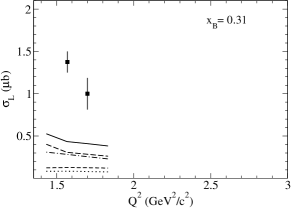
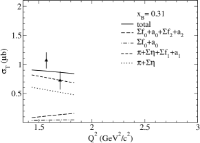
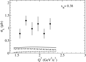
Figure 5: Longitudinal (left panel) and transverse (right panel) cross sections $\sigma_{\scriptscriptstyle L}$ and $\sigma_{\scriptscriptstyle T}$ of $\rho^{0}$ electroproduction as functions of $Q^{2}$. The sum of exchange contributions of all mesons listed in Table 1 is shown by solid lines. The sum of scalar meson contributions (dashed-dotted lines) is calculated with a common value of ${g_{\rho f_{0}\gamma}}$=0.25. The sum of contributions of scalar and tensor mesons is shown by long-dashed lines. The sum of pseudoscalar and pseudovector meson contributions is shown by short-dashed lines (the dotted lines show the pseudoscalar meson contributions). Experimental values are the recent CLAS data clashad .

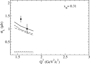
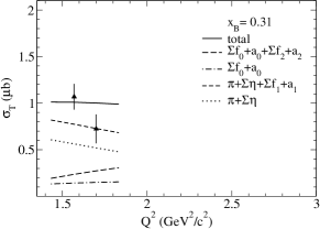
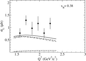
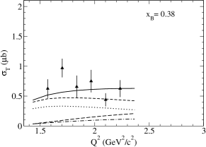
Figure 6: The same results as in Fig. 5 but with an enhanced $\rho f_{0}\gamma$ coupling (${g_{\rho f_{0}\gamma}}$= 1.3) for the two scalar mesons $f_{0}(1370)$ and $f_{0}(1500)$ (and for $a_{0}(1450)$ we use the common rule (41): $g_{\rho a_{0}\gamma}=\frac{1}{3}g_{\rho f_{0}\gamma}$).

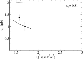
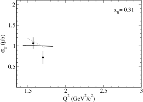
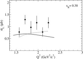
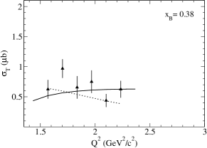
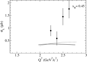
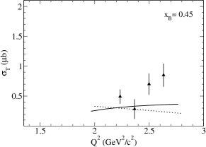
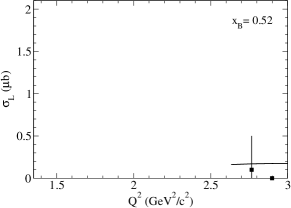
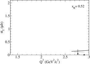
Figure 7: Longitudinal (left panel) and transverse (right panel) cross sections of $\rho^{0}$ electroproduction. The last CLAS data clashad for $x_{\scriptscriptstyle B}=$ 0.31, 0.38, 0.45 and 0.52 are shown in comparison to the theoretical curves. Solid lines correspond to the quasielastic knockout mechanism in which we take into account the full sum of exchange diagrams for intermediate mesons listed in Table 1. The results clashad obtained on the basis of a Regge model of Refs. laget1 ; laget2 ; laget3 ; cano are also shown for comparison (dotted lines).

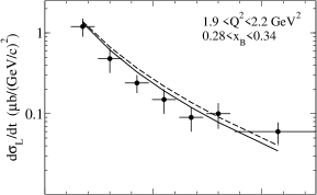
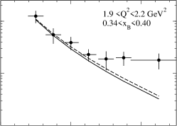
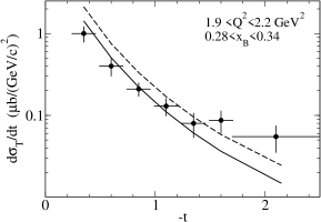
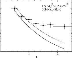
Figure 8: Differential cross sections $d\sigma_{\scriptscriptstyle L}/dt$ (top panel) and $d\sigma_{\scriptscriptstyle T}/dt$ (bottom panel) averaged over intervals 0.28 $<\,x_{\scriptscriptstyle B}\,<$ 0.34 (left) and 0.34 $<\,x_{\scriptscriptstyle B}\,<$ 0.40 (right) at 1.9 $<\,Q^{2}\,<$ 2.2 GeV${}^{2}/c^{2}$ calculated for the same values of ${g_{\rho f_{0}\gamma}}$ as used in Figs. 6 and 7. Comparison with the latest CLAS data clasmor for the respective experimental bins: the solid and dashed lines represent the results of calculations for the cases of destructive and constructive interference between contributions of pseudoscalar ($S_{5}$) and pseudovector ($V_{5}$) mesons respectively (the destructive interference corresponds to the inverse sign of expressions in the last column of Table IV).

Results for the cross sections $\sigma_{\scriptscriptstyle L(T)}$ of $\rho^{0}$ electroproduction in comparison with the data of the CLAS Collaboration clashad are presented in Fig. 5 — separately for transverse (right side) $\sigma_{\scriptscriptstyle T}$ and for longitudinal (left side) $\sigma_{\scriptscriptstyle L}$ parts. For $W\gtrsim$ 2 GeV (i.e. at $x_{\scriptscriptstyle B}=$ 0.31 and 0.38 in the CLAS kinematics) the underlying mechanism of quasi–elastic meson knockout (quark spin–flip in the $M1$ transitions $\gamma_{T}^{*}+\pi^{0}(\eta,\eta^{\prime})\to\rho^{0}$ and change of internal orbital momentum in the $E1$ transitions $\gamma_{T}^{*}+f_{n}(a_{n})\to\rho^{0},\,n=0.1.2$) summed over all meson exchange contributions [see Table I and solid curves in Figs.5-8] is in agreement with the data on $\sigma_{\scriptscriptstyle T}(Q^{2},W)$. However, there is no such agreement for $\sigma_{\scriptscriptstyle L}$. As seen from Fig. 5 for $\sigma_{\scriptscriptstyle T}$ the pion exchange contribution is enhanced due to the interference with the exchanged contributions of other pseudoscalar ($S_{5}=\eta,\eta^{\prime}$) and axial-vector ($V_{5}=f_{1},f_{1}^{\prime},a_{1}$) mesons (curves with short–dashed lines in Figs. 5, 6 and 8) while it is suppressed in $\sigma_{\scriptscriptstyle L}$. It seems that a full explanation of the large value of $\sigma_{\scriptscriptstyle L}$ is based on another reaction mechanism.

We therefore conclude that the mechanism of quasi–elastic meson knockout from the nucleon cloud (with the conversion $M_{5}\to\rho^{0}$) is only weakly realized in the longitudinal cross section. At the same time, electroproduction through scalar $f_{0}$ meson exchange could be connected to another – diffractive – mechanism (see Fig. 4$a$). It seems that in this case the couplings $\rho f_{0}\gamma$ for different $f_{0}$ mesons must be such that their total contribution to the longitudinal part $\sigma_{\scriptscriptstyle L}$ is equivalent to the contribution of the diffractive mechanism. However, as seen from the results displayed in Fig. 5 the total contribution of five $f_{0}$ mesons, further enhanced because of interference with the other mesons $f_{2},a_{0},a_{2}$ of positive parity (curves with long–dashed lines in Fig. 5), is not enough to reproduce the data on $\sigma_{\scriptscriptstyle L}$.

The mismatch of theory with data on $\sigma_{\scriptscriptstyle L}$ is perhaps connected with the fact that for all five $f_{0}$ mesons we use a universal $\rho f_{0}\gamma$ constant $g_{\rho f_{0}\gamma}$ justified only for the radiative decay widths of the lightest scalars: $f_{0}(980)\to\rho^{0}+\gamma$ and $\rho^{0}\to\sigma+\gamma$. The value used here $g_{\rho f_{0}\gamma}=$ 0.25 corresponds to a typical scale of electromagnetic interactions of the $f_{0}$ meson interpreted as a weakly bound molecular $K\bar{K}$ state (in case of $f_{0}(980)$) lyub ; kalash1 or as coupled channel state $\pi\bar{\pi}+q\bar{q}$ with a dominant $\pi\bar{\pi}$ component (in case of the $\sigma=f_{0}(600)$) sigma . Then there must be further scalar states with the $q\bar{q}$ component as the dominant one. In many studies (see, e.g. kalash2 ; kalash3 ; lyub ; torn ; giac ) the heavy scalar mesons $f_{0}(1370)$, $f_{0}(1500)$ and $f_{0}(1710)$ are interpreted as either $q\bar{q}$ ${}^{3}P_{0}$ states or as a mixed state including an additional glueball $G_{\scriptscriptstyle J},\,J=0$ with mass $\sim$ 1.7 GeV according to lattice calculations  glu .

In the classification of the scalar mesons we follow the $SU(3)_{\scriptscriptstyle F}\times O(3)$ scheme of Table I. We adopt the view that the lowest scalar nonet [$\sigma(600)$, $f_{0}(980)$, $a_{0}(980)$, $\kappa(800)$] is described by four-quark(antiquark) $S$-wave configurations $q^{2}\bar{q}^{2}$ which are strongly coupled to the open 2$\pi$, 2$K$ and $\pi K$ channels. For the lowest-lying ${}^{3}P_{0}$ nonet of the $q\bar{q}$ system we use use the scalar states with their masses close to the averaged mass of the other ${}^{3}P_{J=1,2}$ nonets [i.e. to the masses of $f_{1}(1285)$, $f_{1}^{\prime}(1420)$, $f_{2}(1270)$, $f^{\prime}_{2}(1525)$, …, etc.]. Since the ${}^{3}P_{0}$ nonet can accomodate only two isoscalar-scalar $f_{0}$ configurations only two of the three observed resonances, $f_{0}(1370)$, $f_{0}(1500)$ and $f_{0}(1710)$, can be described as quarkonium states. In this case we follow the view giac that these $f_{0}$ states result from the mixing of two scalar-isoscalar $q\bar{q}$ states and an additional isosingulet glueball configuration predicted to reside in this mass regime. It should be noted that our final results for the $\sigma_{L}$ and $d\sigma_{L}/dt$ cross sections are not very sensitive to the detailed mixing scheme residing in this $f_{0}$ sector. Out of the three mesons $f_{0}(1370)$, $f_{0}(1500)$ and $f_{0}(1710)$ we may take any two and treat them in the meson exchange diagrams as if they were quarkonium states. Here, for simplicity, we take the two lowest scalars $f_{0}(1370)$ and $f_{0}(1500)$.

An estimate of the radiative decays of ${}^{3}P_{0}$ quarkonia states done in Refs. kalash1 ; kalash2 shows that the decay width $f_{0}\to\rho^{0}+\gamma$ is rather large with $\Gamma_{f_{0}\to\rho\gamma}=$ 125 KeV assuming a mass of $M_{f_{0}}=$ 0.98 GeV. This means that the coupling constant should have the value $g_{\rho f_{0}\gamma}=$ 1.3, i.e. about five times larger than the value used in the calculations. Starting with this alternative estimate of the coupling constant we recalculated the cross sections $\sigma_{\scriptscriptstyle L}$ and $\sigma_{\scriptscriptstyle T}$ substituting for the cases of $f_{0}(1370)$ and $f_{0}(1500)$ the value $g_{\rho f_{0}\gamma}=$ 1.3 instead of $g_{\rho f_{0}\gamma}=$ 0.25. Here we suppose that the true quarkonia states lie above $\sim$ 1.2 - 1.3 GeV (and thus $f_{0}(980)$ is not a ${}^{3}P_{0}$ quarkonium state), but the behavior of the quarkonia wave function at the origin $R_{\bar{q}q}(r\to 0)$ (which defines the value of $g_{\rho f_{0}\gamma}$) does not change significantly if the mass of the $q\bar{q}$ system used in calculation of the $f_{0}\to\rho_{0}\gamma$ branching will increase from 0.98 GeV to 1.4 – 1.5 GeV.

In Fig. 6 we present the results of this recalculation (the notations are the same as in Fig. 5). The influence of the change of couplings on $\sigma_{\scriptscriptstyle T}$ is negligible consistent with a relatively small contribution of $f_{0}$ exchanges to $\sigma_{\scriptscriptstyle T}$. At the same time the longitudinal cross section $\sigma_{\scriptscriptstyle L}$ is increased considerably and now theoretical curves shown in Fig. 6 are in good agreement with the data clashad within experimental errors.

Recall that the CLAS data at $x_{\scriptscriptstyle B}=$ 0.31 and 0.38 correspond to invariant energies $W$ mostly above the resonance region ($W\cong$ 2 – 2.2 GeV). At lower energies (i.e. at $x_{\scriptscriptstyle B}=$ 0.45 and 0.52 in the CLAS data) theoretical predictions failed to explain the data (Fig. 7). It is possible that the enhancements of the cross sections observed in the region $W\cong$ 1.95 – 2 GeV (this region corresponds to $Q^{2}\cong$ 2.4 - 2.6 GeV${}^{2}/c^{2}$ at fixed $x_{\scriptscriptstyle B}=$ 0.45 in Fig. 7) are consistent with some high-mass baryon resonances. A similar enhancement is also seen in $\sigma_{\scriptscriptstyle T}$ at $x_{\scriptscriptstyle B}=$ 0.38 near $Q^{2}\cong$ 1.7 – 1.8 GeV${}^{2}/c^{2}$ (i.e. near $W\approx$ 1.95 GeV), but unfortunately the experimental uncertainties (especially for $\sigma_{\scriptscriptstyle L}$) are too large in this region. It is interesting to note that our theoretical curves represented in Fig. 7 for all the kinematical region of the CLAS experiment are well correlated (with only one exception for $\sigma_{\scriptscriptstyle L}$ at $x_{\scriptscriptstyle B}=$ 0.31) with the theoretical curves of Ref. clashad obtained on the basis of a Regge model laget1 ; laget2 ; laget3 ; cano .

The new published CLAS data at electron beam energy $E_{e}=$ 5.754 GeV with full information on differential cross sections clasmor allow a more detailed test of our results. In the region of quasi–elastic knockout $|t-t_{min}|\lesssim$ (0.2 - 0.3) GeV${}^{2}/c^{2}$ these results can be considered as predictions and can be used in the analysis of differential cross sections. In Fig.. 8 we show the results for $d\sigma_{\scriptscriptstyle T}(t,W,Q^{2})/dt$ and $d\sigma_{\scriptscriptstyle L}(t,W,Q^{2})/dt$ calculated in the kinematics above the resonance region ($W=$ 2 – 2.4 GeV, $Q^{2}=$ 1.9 – 2.2 GeV${}^{2}/c^{2}$) using enhanced values for $g_{\rho f_{0}\gamma}$ as done for the satisfactory description of $\sigma_{\scriptscriptstyle L,T}$ (Figs. 6 – 7). The transverse cross section $d\sigma_{\scriptscriptstyle T}/dt$ largely depends on the sign of the interference term between pseudoscalar- and pseudovector-meson exchange contributions (the last column of Table IV), and thus we show in Fig. 8 two cases: destructive (solid lines) and constructive (dashed lines) interference of the $S_{5}$ and $V_{5}$ contributions. As can be seen from Fig. 8 the variant with destructive interference correlates well with the CLAS data on both $d\sigma_{\scriptscriptstyle L}/dt$ and $d\sigma_{\scriptscriptstyle T}/dt$ at small $|t|$ close to the quasi–elastic knockout region. For larger values of $|t|\gtrsim$ 1 GeV our prediction underestimates the data, but this deviation may not greatly change the integrated cross sections $\sigma_{\scriptscriptstyle L/T}$. For this reason, our model predictions, originally fitted to the old CLAS data on the integrated cross sections $\sigma_{\scriptscriptstyle L/T}$, also succeed in a satisfactory description of the new data on $d\sigma_{\scriptscriptstyle L/T}/dt$ clasmor .

The full analysis of the new CLAS data clasmor will be presented in its own right in a separate forthcoming paper. The analysis of this new high-precision experimental information in terms of the above model could clarify the role of scalar mesons in the $\rho^{0}$ electroproduction and, finally, could give definite constraints on the free parameters of the effective Lagrangians: coupling constants and form factors.

We also should comment on the possible role of the “non-correlated” two-pion exchange mechanism not considered here. The explicit contribution of the three-pion box diagram to the $\rho^{0}$ photoproduction was studied in Ref. oh (note that the meson exchange parameters used in Ref. oh are practically the same as in the present model). The calculations performed for values of $E_{\gamma}=$ 2.8, 3.28, 3.55 and 3.82 GeV shown that the contribution of this mechanism to the differential cross section becomes comparable to other contributions only for the very forward and backward angles, e.g. for $|t|\lesssim$ 0.1 – 0.2 GeV${}^{2}/c^{2}$. Recall that the threshold value of $t=t^{0}_{min}$ for the $\rho$ photoproduction is very small ($|t^{0}_{min}|\approx$ 0) when compared to the electroproduction threshold value $t^{Q}_{min}$ at $Q^{2}\gtrsim$ 1.5 – 2 GeV${}^{2}/c^{2}$ (e.g., values of $|t^{Q}_{min}|\gtrsim$ 0.2 – 0.4 GeV${}^{2}/c^{2}$ are characteristic of the CLAS kinematics as can be seen from Fig. 8). Based on the results of Ref. oh we therefore think that the non-correlated two-pion exchange does not significantly change our results at $|t|\gtrsim$ 0.2 – 0.4 obtained for the CLAS kinematics with $|t^{Q}_{min}|\gtrsim$ 0.2 – 0.4 GeV${}^{2}/c^{2}$. But we also plan to perform an exact evaluation of the $2\pi$ contribution to $d\sigma_{\scriptscriptstyle L/T}/dt$ in a full analysis of the new CLAS data.

Appendix A Coefficients $A_{T}$,$B_{T}$,$C_{T}$ ,$D_{T}$

The coefficients $A,\,B,\,C,\,D$ and $E$ in Eqs.(52) and (54) are polynomials in $Q$, $t$ and $W$. In particular, the coefficients $A_{\scriptscriptstyle T}$,$B_{\scriptscriptstyle T}$,$C_{\scriptscriptstyle T}$ and $D_{\scriptscriptstyle T}$ which are rather lengthy and not shown in Table III can be written in the form:

$$A_{\scriptscriptstyle T} = \sum_{n=-2}^{4}\left(\frac{Q}{m_{\scriptscriptstyle N}}\right)^{n}a_{n}(\eta,\xi_{s},\xi_{t}),$$

$$B_{\scriptscriptstyle T} = \sum_{n=-2}^{4}\left(\frac{Q}{m_{\scriptscriptstyle N}}\right)^{n}b_{n}(\eta,\xi_{s},\xi_{t}),\,\dots\,,$$ (59)

where the coefficients $a_{n}$, $b_{n},\,\dots$ are polynomials in three dimensionsless variables:

$$\eta=\frac{-t}{4m_{\scriptscriptstyle N}^{2}},\quad\xi_{s} = \frac{pq}{m_{\scriptscriptstyle N}Q}=\frac{Q}{2m_{\scriptscriptstyle N}x_{\scriptscriptstyle B}},$$

$$\xi_{t} = \frac{kq}{m_{\scriptscriptstyle N}Q}=\frac{Q}{2m_{\scriptscriptstyle N}}+\frac{M_{\rho}^{2}-t}{2m_{\scriptscriptstyle N}Q}.$$ (60)

Here we use the standard designation for Bjorken’s variable $x_{\scriptscriptstyle B}=\frac{Q^{2}}{2pq}$ and introduce relative values $\mu_{\rho}=\frac{m_{\scriptscriptstyle N}}{M_{\rho}}$ and $\mu_{f}=\frac{m_{\scriptscriptstyle N}}{M_{f}}$ to simplify formulas. In terms of these variables the polynomials $a_{n}$, $b_{n}$,$c_{n}$ and $d_{n}$ for $n=$ -2, -1, $\dots$, 4 take the form:

$$a_{-2} = -\frac{64}{9}\eta^{2}(\eta+1)\left(4\eta\mu_{f}^{2}+1\right){}^{2},$$

$$b_{-2} = \frac{64}{9}\mu_{\rho}^{2}\,\eta^{2}(\eta+1)\left(4\eta\mu_{f}^{2}+1\right)^{2},$$

$$c_{-2} = 0,$$

$$d_{-2} = 0;$$ (61)

$$a_{-1} = \frac{256}{9}\eta\left(8\eta^{2}(\eta+1)\mu_{f}^{4}+6\eta(\eta+1)\mu_{f}^{2}+\eta+1\right)\xi_{t},$$

$$b_{-1} = -\frac{32}{9}\xi_{t}\eta\left(4\eta\mu_{f}^{2}+1\right)\left\{4\left[8\eta(\eta+1)\mu_{\rho}^{2}+\eta+1\right]\mu_{f}^{2}+8(\eta+1)\mu_{\rho}^{2}-3\right\},$$

$$c_{-1} = \frac{128}{3}\eta\left(4\eta\mu_{f}^{2}+1\right)\xi_{t},$$

$$d_{-1} = -\frac{64}{3}\eta\left(4\eta\mu_{f}^{2}+1\right)\xi_{t};$$ (62)

$$a_{0} = -\frac{512}{3}\mu_{f}^{4}\xi_{t}^{2}\eta^{2}(\eta+1)-\frac{128}{9}\mu_{f}^{2}\eta\left[-12\eta\xi_{s}(\xi_{s}-\xi_{t})+\xi_{t}^{2}(6\eta+9)+8\eta(\eta+1)\right]$$

$$- \frac{16}{9}\left(-24\eta\xi_{s}(\xi_{s}-\xi_{t})+\xi_{t}^{2}\left(16+\eta-9\eta^{2}\right)+16\eta(\eta+1)\right),$$

$$b_{0} = \frac{256}{9}\mu_{f}^{4}\eta(\eta+1)\left[4\eta\left(5\xi_{t}^{2}+2\eta\right)\mu_{\rho}^{2}+3\xi_{t}^{2}+2\eta\right]$$

$$+ \frac{128}{9}\mu_{f}^{2}\left\{-2\eta^{2}-\xi_{t}^{2}\eta+6\mu_{\rho}^{2}\eta\left[-2\eta\xi_{s}^{2}+3\eta\xi_{t}\xi_{s}+(2\eta+3)\xi_{t}^{2}+2\eta(\eta+1)\right]+\eta+2\xi_{t}^{2}\right\}$$

$$+ \frac{4}{9}\left\{9\eta\xi_{t}^{2}-75\xi_{t}^{2}-24\eta+4\mu_{\rho}^{2}\left[-24\eta\xi_{s}^{2}+36\eta\xi_{t}\xi_{s}+\left(-9\eta^{2}+4\eta+16\right)\xi_{t}^{2}+16\eta(\eta+1)\right]\right\},$$

$$c_{0} = -\frac{64}{3}\left(8\eta\left(\xi_{t}^{2}+\eta\right)\mu_{f}^{2}+\left(3\eta^{2}\mu_{\rho}^{2}+7\right)\xi_{t}^{2}+2\eta\right),$$

$$d_{0} = \frac{128}{3}\mu_{f}^{2}\eta\left[-\mu_{\rho}^{2}\eta\xi_{t}(2\xi_{s}-\xi_{t})+2\left(\xi_{t}^{2}+\eta\right)\right]+\frac{32}{3}\left[7\xi_{t}^{2}+2\eta+\eta\mu_{\rho}^{2}\xi_{t}\left(-2\xi_{s}+3\eta\xi_{t}+\xi_{t}\right)\right];$$ (63)

$$a_{1} = \frac{512}{9}\mu_{f}^{4}\xi_{t}^{3}\eta(\eta+1)+\frac{128}{9}\mu_{f}^{2}\xi_{t}\left[-12\eta\xi_{s}^{2}+12\eta\xi_{t}\xi_{s}-(\eta-2)\xi_{t}^{2}+8\eta(\eta+1)\right]$$

$$+ \frac{32}{9}\xi_{t}\left[-6\xi_{t}^{2}-24\xi_{s}(\xi_{s}-\xi_{t})+(\eta+1)(16-9\eta)\right],$$

$$b_{1} = -\frac{128}{9}\mu_{f}^{4}\xi_{t}\left[4\mu_{\rho}^{2}\eta(\eta+1)\left(4\xi_{t}^{2}+9\eta\right)+(\eta+1)\left(\xi_{t}^{2}+8\eta\right)\right]$$

$$- \frac{64}{9}\mu_{f}^{2}\left\{2\mu_{\rho}^{2}\left[6\eta\xi_{s}\left(6\xi_{t}^{2}+\eta\right)-24\eta\xi_{s}^{2}\xi_{t}+(4-8\eta)\xi_{t}^{3}+\eta(22\eta+25)\xi_{t}\right]+\xi_{t}\left(-6\xi_{s}^{2}+6\xi_{t}\xi_{s}-3\xi_{t}^{2}+2\eta+8\right)\right\}$$

$$- \frac{8}{9}\mu_{\rho}^{2}\left\{\xi_{t}\left[-36\eta^{2}-3(3\eta+16)\xi_{t}^{2}+52\eta+64-96\xi_{s}^{2}\right]+24\xi_{s}\left(6\xi_{t}^{2}+\eta\right)\right\}-\frac{8}{3}\xi_{t}\left(12\xi_{s}^{2}+3\eta-6\xi_{s}\xi_{t}-25\right),$$

$$c_{1} = \frac{128}{3}\mu_{f}^{2}\xi_{t}\left(\xi_{t}^{2}+4\eta\right)+32\mu_{\rho}^{2}\xi_{t}\eta\left(\xi_{t}^{2}+4\eta\right)+\frac{32}{3}\xi_{t}\left(-12\xi_{s}^{2}-3\xi_{t}^{2}+12\xi_{s}\xi_{t}+28\right),$$

$$d_{1} = \frac{128}{3}\mu_{f}^{2}\mu_{\rho}^{2}(2\xi_{s}-\xi_{t})\eta\left(2\xi_{t}^{2}+\eta\right)-\frac{16}{3}\mu_{\rho}^{2}\xi_{t}\left[(3\eta+4)\xi_{t}^{2}+2\eta(6\eta+1)\right]+\frac{64}{3}\mu_{\rho}^{2}\xi_{s}\left(2\xi_{t}^{2}+\eta\right)$$ (64)

$$- \frac{8}{3}\xi_{t}\left[8\left(\xi_{t}^{2}+4\eta\right)\mu_{f}^{2}-24\xi_{s}^{2}-3\xi_{t}^{2}+18\xi_{s}\xi_{t}+56\right];$$

$$a_{2} = -\frac{64}{9}\mu_{f}^{4}\xi_{t}^{4}(\eta+1)+\frac{32}{9}\mu_{f}^{2}\xi_{t}^{2}\left\{3\left[\xi_{t}^{2}+4\xi_{s}(\xi_{s}-\xi_{t})\right]-8(\eta+1)\right\}-4\mu_{\rho}^{2}\eta\xi_{t}^{2}\left[\xi_{t}^{2}+4\xi_{s}(\xi_{s}-\xi_{t})\right]$$

$$- \frac{16}{3}(2\xi_{s}-\xi_{t})^{2}\left[3\xi_{s}(\xi_{s}-\xi_{t})+3\eta-4\right]-\frac{4}{9}\left(-36\eta^{2}+28\eta+64\right),$$

$$b_{2} = \frac{128}{9}\mu_{f}^{4}(\eta+1)\left[2\mu_{\rho}^{2}\left(\xi_{t}^{4}+8\eta\xi_{t}^{2}+4\eta^{2}\right)+\xi_{t}^{2}+2\eta\right]$$

$$+ \frac{64}{9}\mu_{f}^{2}\left\{2\mu_{\rho}^{2}\left[-3\left(2\xi_{s}^{2}-\xi_{t}^{2}\right)\left(\xi_{t}^{2}+2\eta\right)+8\eta(\eta+1)+\xi_{s}\left(9\xi_{t}^{3}+30\eta\xi_{t}\right)\right]-6\xi_{s}^{2}-3\xi_{t}^{2}+4\eta+6\xi_{s}\xi_{t}+4\right\}$$

$$+ \frac{4}{3}\mu_{\rho}^{2}\xi_{s}^{2}\left(48\xi_{s}^{2}-144\xi_{s}\xi_{t}+129\xi_{t}^{2}+48\eta-64\right)$$

$$+ \frac{4}{9}\mu_{\rho}^{2}\left\{-12\xi_{s}\xi_{t}\left(9\xi_{t}^{2}+18\eta-32\right)+4\left[-9\eta^{2}+9(\eta-4)\xi_{t}^{2}+16(\eta+1)\right]\right\}+\frac{4}{3}\left(24\xi_{s}^{2}+3\eta-12\xi_{s}\xi_{t}-25\right),$$

$$c_{2} = -\frac{128}{3}\mu_{f}^{2}\xi_{t}^{2}-\frac{4}{3}\mu_{\rho}^{2}\left[-9\xi_{t}^{4}+48\xi_{s}\xi_{t}^{3}+48\left(\eta-\xi_{s}^{2}\right)\xi_{t}^{2}+48\eta^{2}\right]-\frac{32}{3}\left(-12\xi_{s}^{2}+12\xi_{t}\xi_{s}-3\xi_{t}^{2}+14\right),$$

$$d_{2} = -\frac{64}{3}\mu_{f}^{2}\mu_{\rho}^{2}\xi_{t}\left[-\xi_{t}^{3}+2\xi_{s}\left(\xi_{t}^{2}+6\eta\right)-6\eta\xi_{t}\right]+\frac{64}{3}\mu_{f}^{2}\xi_{t}^{2}+\frac{4}{3}\left(-48\xi_{s}^{2}-6\xi_{t}^{2}+36\xi_{s}\xi_{t}+56\right)$$ (65)

$$+ \frac{4}{3}\mu_{\rho}^{2}\left[48\xi_{t}\xi_{s}^{3}-96\xi_{t}^{2}\xi_{s}^{2}+\xi_{t}\xi_{s}\left(51\xi_{t}^{2}+24\eta-64\right)-6\xi_{t}^{4}+4(3\eta+8)\xi_{t}^{2}+24\eta^{2}\right];$$

$$a_{3} = 8\eta\mu_{\rho}^{2}\xi_{t}\left(\xi_{t}-2\xi_{s}\right){}^{2},$$

$$b_{3} = -\frac{256}{9}\mu_{f}^{4}\mu_{\rho}^{2}(\eta+1)\xi_{t}\left(\xi_{t}^{2}+2\eta\right)-\frac{64}{3}\mu_{f}^{2}\mu_{\rho}^{2}\xi_{s}\left(-2\xi_{s}\xi_{t}+5\xi_{t}^{2}+4\eta\right)+\frac{128}{9}\mu_{f}^{2}\mu_{\rho}^{2}\xi_{t}\left(3\xi_{t}^{2}+\eta-2\right)$$

$$- \frac{24}{9}\mu_{\rho}^{2}\xi_{s}\left(-24\xi_{s}^{2}+39\xi_{t}\xi_{s}-15\xi_{t}^{2}-12\eta+16\right)-\frac{8}{9}\mu_{\rho}^{2}\xi_{t}\left(9\eta-24\right),$$

$$c_{3} = 8\mu_{\rho}^{2}\xi_{t}\left(-16\xi_{s}^{2}+16\xi_{t}\xi_{s}-3\xi_{t}^{2}+4\eta\right),$$

$$d_{3} = \frac{32}{3}\mu_{f}^{2}\mu_{\rho}^{2}(2\xi_{s}-\xi_{t})\left(3\xi_{t}^{2}+4\eta\right)-\frac{32}{3}\mu_{\rho}^{2}\xi_{s}\left(6\xi_{s}^{2}-15\xi_{t}\xi_{s}-9\xi_{t}^{2}-3\eta+4\right)-\frac{4}{3}\mu_{\rho}^{2}\xi_{t}\left(-9\xi_{t}^{2}+16\right);$$ (66)

$$a_{4} = -4\eta\mu_{\rho}^{2}\left(\xi_{t}-2\xi_{s}\right){}^{2},$$

$$b_{4} = \frac{64}{9}\mu_{f}^{4}\mu_{\rho}^{2}\xi_{t}^{2}(1+\eta)+\frac{32}{3}\mu_{f}^{2}\mu_{\rho}^{2}\xi_{t}(2\xi_{s}-\xi_{t})+4\mu_{\rho}^{2}\xi_{s}(3\xi_{s}-2\xi_{t}),$$

$$c_{4} = 4\mu_{\rho}^{2}\left(16\xi_{s}^{2}-16\xi_{t}\xi_{s}+3\xi_{t}^{2}\right),$$

$$d_{4} = -\frac{32}{3}\mu_{f}^{2}\mu_{\rho}^{2}\xi_{t}(2\xi_{s}-\xi_{t})-4\mu_{\rho}^{2}\left(8\xi_{s}^{2}-7\xi_{t}\xi_{s}+\xi_{t}^{2}\right).$$ (67)

Table I. $SU(3)_{F}\times O(3)$ classification of neutral mesons contributing to the electroproduction of $\rho^{0}$ (the octet-singlet mixing is omitted for simplicity). Quark model (QM) and hadronic molecular (HM) states usually used for description of meson properties are also shown (including a possible scalar glueball $G_{0}$).

$I^{G}(J^{PC})$	QM (${}^{2S+1}L_{J}$) or HM	$SU(3)$ octet states	$SU(3)$ singlet states
$0^{+}(0^{-+})$	${}^{1}\!S_{0}\qquad\quad$	$\eta(540)$	$\eta^{\prime}(958)$
$1^{-}(0^{-+})$	${}^{1}\!S_{0}\qquad\quad$	$\pi(140)$
$0^{+}(0^{++})$	$\qquad\quad K\bar{K},\,2\pi$	$f_{0}(980)$	$f_{0}(600)\equiv\sigma$
$0^{+}(0^{++})$	${}^{3}\!P_{0}\qquad\quad$	$f_{0}(1370)$	$f_{0}(1500)$
$0^{+}(0^{++})$	$\qquad\quad(G_{0})$		$f_{0}(1710)$
$0^{+}(1^{++})$	${}^{3}\!P_{1}\qquad\quad$	$f_{1}(1285)$	$f_{1}^{\prime}(1420)$
$0^{+}(2^{++})$	${}^{3}\!P_{2}\qquad\quad$	$f_{2}(1270)$	$f_{2}^{\prime}(1525)$
$1^{-}(0^{++})$	$\qquad\quad K\bar{K}$	$a_{0}(980)$
$1^{-}(0^{++})$	${}^{3}\!P_{0}\qquad\quad$	$a_{0}(1450)$
$1^{-}(1^{++})$	${}^{3}\!P_{1}\qquad\quad$	$a_{1}(1260)$
$1^{-}(2^{++})$	${}^{3}\!P_{2}\qquad\quad$	$a_{2}(1320)$

Table II. Expressions for the $\rho M\gamma$ and $MNN$ vertices

$M$	$S_{5}\,(\eta,\pi^{0})$	$V_{5}\,(f_{1},a_{1})$	$S\,(f_{0},a_{0})$	$T\,(f_{2},a_{2})$
$\Gamma^{\varkappa,\mu\nu}_{\scriptscriptstyle M}$	$\mbox{-}eg_{\rho{\scriptscriptstyle M}\gamma}\varepsilon^{\mu\nu\alpha\beta}\frac{q_{\alpha}{k^{\prime}}_{\!\!\beta}}{M_{\rho}}\!$	-$eg_{\rho{\scriptscriptstyle M}\gamma}\varepsilon^{\mu\nu\alpha\beta}\frac{{k^{\prime}}^{2}q_{\beta}-q^{2}{k^{\prime}}_{\!\!\beta}}{M_{\rho}^{2}}$	$eg_{\rho{\scriptscriptstyle M}\gamma}\frac{qk^{\prime}}{M_{\rho}}\left(\!g^{\mu\nu}\!-\!\frac{q^{\mu}{k^{\prime}}^{\nu}}{qk^{\prime}}\!\right)$	$\!eg_{\rho{\scriptscriptstyle M}\gamma}\frac{1}{M_{\scriptscriptstyle T}}\!\left[g^{\mu\nu}(q\!+\!k^{\prime})^{\alpha}(q\!+\!k^{\prime})^{\beta}\right.\!$
				$\!\mbox{-}g^{\mu\alpha}\!{k^{\prime}}^{\nu}\!(q\!+\!k^{\prime})^{\beta}\!-\!g^{\mu\beta}{k^{\prime}}^{\nu}\!(q\!+\!k^{\prime})^{\alpha}\!$
				$\!\mbox{-}g^{\nu\alpha}q^{\mu}(q\!+\!k^{\prime})^{\beta}\!-\!g^{\nu\beta}q^{\mu}(q\!+\!k^{\prime})^{\alpha}\!$
				$\left.+2qk^{\prime}(g^{\nu\alpha}g^{\mu\beta}\!+\!g^{\nu\beta}g^{\mu\alpha})\right]$
$\Gamma_{\scriptscriptstyle M}^{\varkappa}$	$\frac{g_{\scriptscriptstyle MNN}}{2m_{N}}\!\!\not\!k\gamma^{5}$	$g_{\scriptscriptstyle MNN}\gamma^{\alpha}\gamma^{5}$	$g_{\scriptscriptstyle MNN}$	$\frac{g_{\scriptscriptstyle MNN}}{m_{N}}[(p\!+\!p^{\prime})^{\alpha}\gamma^{\beta}\!+\!(p\!+\!p^{\prime})^{\beta}\gamma^{\alpha}]$

Table III. Coefficients $A_{\scriptscriptstyle M}$, $B_{\scriptscriptstyle M}$, $C_{\scriptscriptstyle M}$, $D_{\scriptscriptstyle M}$ and $E_{\scriptscriptstyle M}$ of Eq. (52)

$M$	$S_{5}\,(\eta,\pi^{0})$	$V_{5}\,(f_{1},a_{1})$	$S\,(f_{0},a_{0})$	$T(f_{2},a_{2}\!)\!$
$A_{\scriptscriptstyle M}$	$-\eta\left(\xi_{t}^{2}\!-4\eta\right)\!$	$2-\xi_{s}^{2}+\xi_{s}\xi_{t}-(\xi_{t}^{2}-4\eta)\frac{m_{N}^{2}}{M_{\rho}^{2}}\left[\frac{m_{N}^{2}}{Q^{2}}(\!1+\eta)+\frac{2M_{\rho}^{2}}{M_{V5}^{2}}\left(1+2\eta\frac{m_{N}^{2}}{M_{V5}^{2}}\right)\right]$	$(1+\eta)\!\left(\!\frac{M_{\rho}^{2}}{m_{N}^{2}}-\xi_{t}^{2}+4\eta\!\right)\!\!$	${}^{*})$
		$+z^{2}(1+\eta)\left[\frac{4m_{N}^{2}}{Q^{2}}\eta-(\xi_{t}^{2}-4\eta)\frac{m_{N}^{2}}{M_{\rho}^{2}}\right]+z\frac{2m_{N}}{Q}\left[2\eta\xi_{s}-(1+2\eta)\xi_{t}\right]$
$B_{\scriptscriptstyle M}$	$\eta$	$\frac{m_{N}^{2}}{M_{\rho}^{2}}\!\left[\frac{m_{N}^{2}}{Q^{2}}(1+\eta)+\frac{2M_{\rho}^{2}}{M_{\scriptscriptstyle V5}^{2}}\left(1+\!2\eta\frac{m_{N}^{2}}{M_{\scriptscriptstyle V5}^{2}}\right)\right]+z^{2}\!\left[\frac{m_{N}^{2}}{Q^{2}}(1+\!2\eta)+\frac{m_{N}^{2}}{M_{\rho}^{2}}(1+\eta)\right]\!$	$1+\eta$	${}^{*})$
$C_{\scriptscriptstyle M}$	$0$	$1+z^{2}\frac{4m_{N}^{2}}{Q^{2}}\eta-z\frac{2m_{N}}{Q}\xi_{t}$	$0$	${}^{*})$
$D_{\scriptscriptstyle M}$	$0$	$-\frac{1}{2}-z^{2}\,\frac{2m_{N}^{2}}{Q^{2}}\eta+z\frac{m_{\scriptscriptstyle N}}{Q}\xi_{s}$	$0$	${}^{*})$
$E_{\scriptscriptstyle M}$	$0$	$\frac{m_{N}^{4}}{M_{\rho}^{2}Q^{2}}(1+z^{2})$	$0$	$0$
$\widetilde{g}_{\rho{\scriptscriptstyle M}\gamma}\!$	$\frac{m_{\scriptscriptstyle N}}{M_{\rho}}g_{\rho{{\scriptscriptstyle S}_{5}}\gamma}$	$\frac{Q^{2}}{zM_{\rho}^{2}}g_{\rho{{\scriptscriptstyle V}_{5}}\gamma}\,,\quad z=\frac{Q^{2}}{M_{\rho}^{2}+Q^{2}}$	$\frac{m_{\scriptscriptstyle N}}{M_{\rho}}g_{\rho{\scriptscriptstyle S}\gamma}$	$\frac{m_{\scriptscriptstyle N}}{M_{\scriptscriptstyle T}}g_{\rho{\scriptscriptstyle T}\gamma}$
${\cal N}_{\scriptscriptstyle M}$	$\,\,e\widetilde{g}_{\rho{\scriptscriptstyle M}\gamma}g_{\scriptscriptstyle MNN}{\cal F}_{\rho{\scriptscriptstyle M}\gamma}(Q^{2},t){\cal F}_{\scriptscriptstyle MNN}(t)\,2m_{\scriptscriptstyle N}Q/(M_{\scriptscriptstyle M}^{2}-t)$

${}^{*})$ see $A_{\scriptscriptstyle T}$,$B_{\scriptscriptstyle T}$, $C_{\scriptscriptstyle T}$ and $D_{\scriptscriptstyle T}$ in Appendix

Table IV. $A_{{\scriptscriptstyle MM}^{\prime}}$, $B_{{\scriptscriptstyle MM}^{\prime}}$, $C_{{\scriptscriptstyle MM}^{\prime}}$, $D_{{\scriptscriptstyle MM}^{\prime}}$ and $E_{{\scriptscriptstyle MM}^{\prime}}$ of Eq. (54)

$MM^{\prime}$	$ST$	$S_{5}V_{5}$
$A_{{\scriptscriptstyle MM}^{\prime}}$	$-8\left(\frac{Q}{m_{N}}\!-\!\xi_{t}\right)\!\left\{\frac{Q}{m_{N}}(2\xi_{s}\!-\!\xi_{t})^{2}-\frac{4}{3}(1\!+\!\eta)\left[2\left(\frac{Q}{m_{N}}\!-\!\xi_{t}\right)\right.\right.$
	$\left.\left.+\eta\frac{m_{N}}{Q}+\frac{m_{N}^{2}}{M_{\scriptscriptstyle T}^{2}}\frac{Q}{m_{N}}\left(\xi_{t}\!-\!2\eta\frac{m_{N}}{Q}\right)^{2}\right]\right\}$	$-(\xi_{t}^{2}\!-\!4\eta)\left(1\!+\frac{4m_{\scriptscriptstyle N}^{2}}{M_{\scriptscriptstyle V5}^{2}}\!\eta\right)$
$B_{{\scriptscriptstyle MM}^{\prime}}$	$-8\left(\frac{Q}{m_{N}}\!-\!\xi_{t}\right)\left[\xi_{s}-2\frac{Q}{m_{N}}+\frac{4}{3}(1\!+\!\eta)\frac{m_{N}^{2}}{M_{\scriptscriptstyle T}^{2}}\right]$	$1\!+\frac{4m_{\scriptscriptstyle N}^{2}}{M_{\scriptscriptstyle V5}^{2}}\!\eta$
$C_{{\scriptscriptstyle MM}^{\prime}}$	$32\left(\frac{Q}{m_{N}}\!-\!\xi_{t}\right)^{2}$	$0$
$D_{{\scriptscriptstyle MM}^{\prime}}$	$8\left(\frac{Q}{m_{N}}\!-\!\xi_{t}\right)\left[2\xi_{s}+\xi_{t}-2\frac{Q}{m_{N}}\right]$	$0$
$E_{{\scriptscriptstyle MM}^{\prime}}$	$0$	$0$

References

- (1) C. Hadjidakis et al. (CLAS Collaboration), Phys. Lett. B 605, 256 (2005).
- (2) S. A. Morrow et al. (CLAS Collaboration), Eur. Phys. J. A 39, 5 (2009).
- (3) M. Battaglieri et al. (CLAS Collaboration), Phys. Rev. Lett. 87, 172002 (2001); M. Battaglieri et al. (CLAS Collaboration), Phys. Rev. Lett. 90, 022002 (2003).
- (4) G. M. Huber et al. (Jefferson Lab. Collab.), Phys. Rev. C 78, 045203 (2008).
- (5) T. Horn et al. (Jefferson Lab. Collab.), Phys. Rev. Lett. 97, 192001 (2006).
- (6) J. Volmer et al. (Jefferson Lab. Collab.), Phys. Rev. Lett. 86, 1713 (2001)
-
(7)
A. Faessler, T. Gutsche, V. E. Lyubovitskij and
I. T. Obukhovsky, Phys. Rev. C 76, 025213 (2007). - (8) D. G. Cassel et al., Phys. Rev. D 24, 2787 (1981).
- (9) B. Renner, Nucl. Phys. B 30, 634 (1971); B. Renner, Phys. Lett. B 33, 599 (1970).
- (10) Y. S. Oh and T. S. H. Lee, Phys. Rev. C 69, 025201 (2004).
- (11) M. Guidal and S. Morrow, Proceedings of the International Workshop Exclusive reactions at high momentum transfer, Jefferson Labaratory, Newport-News, Virginia, USA, May 21-24 2007 (World Scientific, 2008) ISBN 9812796940, arXiv:0711.3743 [hep-ph].
- (12) M. M. Kaskulov, K. Gallmeister and U. Mosel, Phys. Rev. D 78, 114022 (2008); M. M. Kaskulov and U. Mosel, Phys. Rev. C 80, 028202 (2009).
- (13) J. M. Laget and R. Mendez-Galain, Nucl. Phys. A 581, 397 (1995).
- (14) M. Guidal, J. M. Laget and M. Vanderhaeghen, Nucl. Phys. A 627, 645 (1997).
-
(15)
J. M. Laget,
Phys. Rev. D 70, 054023 (2004);
J. M. Laget, Phys. Lett. B 489, 313 (2000); J. M. Laget, Nucl. Phys. A 699, 184c (2002). - (16) F. Cano and J. M. Laget, Phys. Lett. B 551, 317 (2003) [Erratum-ibid. B 571, 250 (2003)].
- (17) A. Donnachie and P. V. Landshoff, Nucl. Phys. B 244, 322 (1984); A. Donnachie and P. V. Landshoff, arXiv:0803.0686 [hep-ph].
- (18) I. T. Obukhovsky, D. Fedorov, A. Faessler, T. Gutsche and V. E. Lyubovitskij, Phys. Lett. B 634, 220 (2006).
- (19) V. G. Neudatchin, I. T. Obukhovsky, L. L. Sviridova and N. P. Yudin, Nucl. Phys. A 739, 124 (2004).
- (20) M. N. Achasov et al. (SND Collab.), Phys. Lett. B 537, 201 (2002).
- (21) C. Amsler et al. [Particle Data Group], Phys. Lett. B 667, 1 (2008).
- (22) Yu. Kalashnikova, A. E. Kudryavtsev, A. V. Nefediev, J. Haidenbauer and C. Hanhart, Phys. Rev. C 73, 045203 (2006).
- (23) F. E. Close, A. Donnachie and Yu. S. Kalashnikova, Phys. Rev. D 67, 074031 (2003).
- (24) B. Friman and M. Soyeur, Nucl. Phys. A 600, 477 (1996).
-
(25)
L. S. Kisslinger,
Nucl. Phys. A 629, 30c (1998);
L. S. Kisslinger and W. H. Ma, Phys. Lett. B 485, 367 (2000); L. S. Kisslinger and M. B. Johnson, Phys. Lett. B 523, 127 (2001). - (26) G. V. Efimov and M. A. Ivanov, The Quark Confinement Model of Hadrons, (IOP Publishing, Bristol Philadelphia, 1993).
- (27) M. A. Ivanov, M. P. Locher and V. E. Lyubovitskij, Few Body Syst. 21, 131 (1996); M. A. Ivanov, V. E. Lyubovitskij, J. G. Körner and P. Kroll, Phys. Rev. D 56, 348 (1997) [arXiv:hep-ph/9612463].
- (28) A. Faessler, T. Gutsche, M. A. Ivanov, V. E. Lyubovitskij and P. Wang, Phys. Rev. D 68, 014011 (2003).
- (29) T. Branz, T. Gutsche and V. E. Lyubovitskij, Eur. Phys. J. A 37, 303 (2008).
- (30) M. Kirchbach and L. Tiator, Nucl. Phys. A 604, 385 (1996).
- (31) A. I. Titov, T. S. Lee, H. Toki and O. Streltsova, Phys. Rev. C 60, 035205 (1999).
- (32) T. Hatsuda, Nucl. Phys. B 329, 376 (1990).
- (33) R. N. Cahn, Phys. Rev. D 35, 3342 (1987).
- (34) F. E. Close, A. Donnachie and Yu. S. Kalashnikova, Phys. Rev. D 65, 092003 (2002).
- (35) T. Bolton et al., Phys. Lett. B 278, 495 (1992).
- (36) M. Kirchbach and D. O. Riska, Nucl. Phys. A 594, 419 (1995); M. Kirchbach, L. Tiator, S. Neumeier and S. Kamalov, arXiv:nucl-th/9609021.
- (37) J. R. Ellis and M. Karliner, Phys. Lett. B 313, 131 (1993).
- (38) J. P. Santoro et al. (CLAS Collaboration), Phys. Rev. C 78, 025210 (2008).
- (39) E. van Beveren, T. A. Rijken, K. Metzger, C. Dullemond, G. Rupp and J. E. Ribeiro, Z. Phys. C 30, 615 (1986); E. van Beveren and G. Rupp, Eur. Phys. J. A 31, 468 (2007).
- (40) N. A. Tornqvist and M. Roos, Phys. Rev. Lett. 76, 1575 (1996).
-
(41)
F. Giacosa, T. Gutsche, V. E. Lyubovitskij and
A. Faessler, Phys. Rev. D 72, 094006 (2005). - (42) Y. Chen et al., Phys. Rev. D 73, 014516 (2006); J. Sexton, A. Vaccarino and D. Weingarten, Nucl. Phys. Proc. Suppl. 47, 128 (1996).