Quintessence with quadratic coupling to dark matter

Abstract

We introduce a new form of coupling between dark energy and dark matter that is quadratic in their energy densities. Then we investigate the background dynamics when dark energy is in the form of exponential quintessence. The three types of quadratic coupling all admit late-time accelerating critical points, but these are not scaling solutions. We also show that two types of coupling allow for a suitable matter era at early times and acceleration at late times, while the third type of coupling does not admit a suitable matter era.

I Introduction

Cosmological observations strongly suggest that the expansion rate of the universe is accelerating and that matter in the universe is dominated by non-baryonic cold dark matter (see e.g. Dunkley et al. (2008)). However, what exactly causes this acceleration is not well understood, and one of the main challenges of modern cosmology is to understand the nature of this mysterious dark energy. The existence of some form of dark matter is long known, as implied by the flattened galactic rotation curves observed by Zwicky as early as 1933. Several experiments have been carried out (see, for example Collaboration (2009)) in search of candidate dark matter particles. The fact that dark matter only interacts weakly with standard matter means that it is difficult to detect such particles directly. Neither dark energy nor dark matter have been detected directly. Only the total dark sector energy-momentum tensor is known from its combined gravitational effect. In order to separate the two components, we have to assume a model for them. It is possible that these components interact with each other, while not being coupled to standard model particles. Such a possibility can lead to new approaches to the coincidence problem (“how do dark matter and dark energy attain the same order-of-magnitude value at the right time to allow for the observed large-scale structure?”). It can also produce interesting new features in large-scale structure, such as a large-scale gravitational bias Amendola and Tocchini-Valentini (2002) and a violation of the weak equivalence principle by dark matter on cosmological scales Koyama et al. (2009).

In this paper we study a class of cosmological models with interactions in the dark sector. Various models of the coupling between dark energy and dark matter have been proposed and investigated (see, e.g. Wetterich (1995); Amendola (1999); Billyard and Coley (2000); Zimdahl and Pavon (2001); Farrar and Peebles (2004); Chimento et al. (2003); Olivares et al. (2005); Sadjadi and Alimohammadi (2006); Guo et al. (2007); Kim et al. (2007); Boehmer et al. (2008); He and Wang (2008); Chen et al. (2008); Quartin et al. (2008); Pereira and Jesus (2009); Quercellini et al. (2008); Valiviita et al. (2008)). We consider only the background dynamics – for cosmological perturbations of coupled dark energy models, see e.g. Amendola et al. (2003); Koivisto (2005); Olivares et al. (2006); Mainini and Bonometto (2007); Bean et al. (2008a); Valiviita et al. (2008); Vergani et al. (2008); Pettorino and Baccigalupi (2008); Schaefer (2008); Schaefer et al. (2008); La Vacca and Colombo (2008); He et al. (2009a); Bean et al. (2008b); Corasaniti (2008); Chongchitnan (2009); Jackson et al. (2009); Gavela et al. (2009); La Vacca et al. (2009); He et al. (2009b); Caldera-Cabral et al. (2009a); He et al. (2009c); Koyama et al. (2009); Valiviita et al. (2009); Majerotto et al. (2009).

There is no fundamental theory that selects a specific coupling in the dark sector, and therefore any coupling model will necessarily be phenomenological, although some models will have more physical justification than others. Here we analyse the background dynamics for a new model of coupling. This model improves the one previously introduced in Boehmer et al. (2008); Valiviita et al. (2008), which was motivated by simple models of inflaton decay during reheating and of curvaton decay to radiation.

The background description of a coupled model with quintessence dark energy density $\rho_{\varphi}$ and dark matter density $\rho_{c}$ is given by the energy balance equations

$$\dot{\rho}_{c} =-3H\rho_{c}+Q_{c}\,,$$ (1)

$$\dot{\rho}_{\varphi} =-3H(1+w_{\varphi})\rho_{\varphi}+Q_{\varphi}\,,\qquad Q_{\varphi}=-Q_{c}:=Q\,.$$ (2)

Here $Q_{A}$ is the rate of energy transfer to species $A$. It follows that

$$Q~{}\left\{\begin{array}[]{l}>0\\ <0\end{array}\right.\quad\Rightarrow\quad\mbox{energy transfer is}~{}\left\{\begin{array}[]{l}\mbox{dark matter $\to$ dark energy}\\ \mbox{dark energy $\to$ dark matter}\end{array}\right.$$ (3)

The dark energy equation of state parameter is

$$w_{\varphi}:=\frac{p_{\varphi}}{\rho_{\varphi}}=\frac{\frac{1}{2}\dot{\varphi}^{2}-V(\varphi)}{\frac{1}{2}\dot{\varphi}^{2}+V(\varphi)}\,.$$ (4)

The modified Klein-Gordon equation follows from Eq. (2) as

$$\ddot{\varphi}+3H\dot{\varphi}+\frac{dV}{d\varphi}=\frac{Q}{\dot{\varphi}}\,.$$ (5)

For quintessence with an exponential potential,

$$V(\varphi)=V_{0}\exp\left(-\kappa\lambda\varphi\right)\,,\qquad\kappa^{2}:=8\pi G\,,$$ (6)

where $\lambda$ is a dimensionless parameter and $V_{0}>0$. We neglect the radiation and therefore the evolution equations are

$$\dot{\rho}_{b} =-3H\rho_{b}\,,$$ (7)

$$\dot{H} =-\frac{\kappa^{2}}{2}\left[\rho_{c}+\rho_{b}+\dot{\varphi}^{2}\right]\,,$$ (8)

where baryons $\rho_{b}$ are not coupled to the dark sector. The Friedman constraint is

$$H^{2}=\frac{\kappa^{2}}{3}\left(\rho_{c}+\rho_{b}+\rho_{\varphi}\right).$$ (9)

We define effective equation of state parameters for the dark components which describe the equivalent uncoupled model in the background: $\dot{\rho}_{c}+3H(1+w_{c,\text{eff}})\rho_{c}=0$, $\dot{\rho}_{\varphi}+3H(1+w_{\varphi,\text{eff}})\rho_{\varphi}=0$. By Eqs. (1) and (2),

$$w_{c,\text{eff}}=\frac{Q}{3H\rho_{c}}\,,\qquad w_{\varphi,\text{eff}}=w_{\varphi}-\frac{Q}{3H\rho_{\varphi}}\,.$$ (10)

II New model of dark sector coupling

In Boehmer et al. (2008); Valiviita et al. (2008) a model of the form

$$Q=\Gamma\rho_{c},$$ (11)

was introduced, with $\Gamma$ constant. The motivation for this form of interaction is that, for $\Gamma>0$, the same $Q$ is used for simple models of: (1) the decay of an inflaton field to radiation during reheating Turner (1983), (2) the decay of dark matter into radiation Cen (2000), (3) the decay of a curvaton field into radiation Malik et al. (2003), (4) the decay of super-heavy dark matter particles into a scalar field Ziaeepour (2004).

We consider this coupling to be better motivated than alternatives of the form $Q=\alpha H\rho_{c}$ – which are designed for mathematical simplicity, since they lead to the same number of dimensions of the phase space (two) as the uncoupled case. The coupling in Eq. (11) is not designed for mathematical simplicity, but is chosen as a physically simple form of decay law. It leads to a three-dimensional phase space. This new phase can be compactified Boehmer et al. (2008), as in the two-dimensional case, but great care is required in analysing the stability properties of the resulting dynamical system. The stability matrix contains singular eigenvalues as one approaches the critical points. In Boehmer et al. (2008) we developed the required machinery to overcome these problems and were able to present a complete phase space analysis. Our techniques are readily applicable to more general couplings.

Simple decay laws of the form in Eq. (11) fail to reflect the feature that interactions are typically determined by both energy densities. We therefore consider the natural first extension Eq. (11) to a quadratic form

$$Q=\mathcal{A}\rho_{\varphi}^{2}+\mathcal{B}\rho_{c}^{2}+\mathcal{C}\rho_{c}\rho_{\varphi}\,,$$ (12)

where $\mathcal{A}$, $\mathcal{B}$ and $\mathcal{C}$ are coupling constants. We define dimensionless coupling constants as

$$\alpha=\mathcal{A}{H_{0}}\,,~{}~{}\beta=\mathcal{B}{H_{0}}\,,~{}~{}\gamma=\mathcal{C}{H_{0}}\,.$$ (13)

The Friedman constraint (9) in dimensionless form becomes

$$\Omega_{c}+\Omega_{\varphi}=1\,,\qquad\Omega:=\frac{\kappa^{2}\rho}{3H^{2}}\,,$$ (14)

where we neglect the baryons, and the total equation of state parameter is given by

$$\dot{\rho}_{\text{tot}}+3H(1+w_{\text{tot}})\rho_{\text{tot}}=0\,,$$ (15)

$$w_{\text{tot}}:=\frac{p_{\text{tot}}}{\rho_{\text{tot}}}=\frac{p_{\varphi}}{\rho_{\varphi}+\rho_{c}}=w_{\varphi}\Omega_{\varphi}\,.$$ (16)

The condition for acceleration is $w_{\text{tot}}<-1/3$. A phantom field with $w_{\varphi}<-1$ violates the dominant energy condition, $\rho\geq|p|$. We therefore assume that $w_{\varphi}>-1$, thereby excluding phantom models with negative kinetic energy.

We introduce the dimensionless variables $x,y$, as in the uncoupled case Copeland et al. (1998), where

$$x^{2}:=\frac{\kappa^{2}\dot{\varphi}^{2}}{{6}H^{2}}\,,\qquad y^{2}:=\frac{\kappa^{2}{V}}{{3}H^{2}}\,.$$ (17)

Then $y\geq 0$ because of the positivity of the potential energy, and Eq. (14) implies that

$$0\leq\Omega_{\varphi}=x^{2}+y^{2}\leq 1\,.$$ (18)

In the new variables, the equation of state parameters are

$$w_{\varphi}=\frac{x^{2}-y^{2}}{x^{2}+y^{2}}\,,\qquad w_{\text{tot}}=x^{2}-y^{2}\,.$$ (19)

The Hubble evolution equation may be written as

$$\frac{\dot{H}}{H^{2}}=-\frac{3}{2}(1+x^{2}-y^{2})\,.$$ (20)

As already indicated, it turns out that the resulting evolution equations do not allow a two-dimensional representation of this model, since we cannot eliminate $H$ from the energy balance equations (1) and (2), using only the variables $x(N),y(N)$, where we use $N=\log(a)$ as the independent variable. Equation (20) must therefore be incorporated into the dynamical system. We do this via a new variable $z$, chosen so as to maintain compactness of the phase space

$$z=\frac{H_{0}}{H+H_{0}}\,.$$ (21)

Thus $0\leq z\leq 1$, and the compactified phase space now corresponds to a half-cylinder of unit height and radius Boehmer et al. (2008). The top of this half-cylinder is defined by $z=1$ and it turns out that the equations become singular as $z\to 1$. Therefore, care is required in order to analyse the resulting dynamical system.

It is evident that the quadratic and higher-order couplings can be treated in a similar fashion, for instance one could consider a coupling of the form $Q=\mu\rho_{\varphi}^{3}\rho_{c}$. The most general model is of the form

$$Q=\sum\limits_{m,n}q_{mn}\rho_{c}^{m}\rho_{\varphi}^{n}\,,$$ (22)

where $m,n$ are non-negative integers. The matrix $q_{mn}$ is arbitrary except for the condition $q_{00}=0$. Note that $q_{mn}$ has no a priori symmetry properties and is not necessarily a square matrix. The linear model in Eq. (11) was extended to the most general linear model, $Q=-(\Gamma_{c}\rho_{c}+\Gamma_{\phi}\rho_{\phi})$ in Caldera-Cabral et al. (2009b). The linear and quadratic models lead to

$$(q)_{mn}=\begin{pmatrix}0&\Gamma_{\phi}\\ \Gamma_{c}&0\end{pmatrix},~{}~{}~{}(q)_{mn}=\begin{pmatrix}0&0&\mathcal{A}\\ 0&\mathcal{C}&0\\ \mathcal{B}&0&0\end{pmatrix}.$$ (23)

III Dynamical analysis

In this section we analyse the three particular cases when two of the interaction terms are equal to zero. Two of these models allow for a standard matter era, but the model with $\mathcal{A}=\mathcal{C}=0$ does not allow it. Then we combine the models $\mathcal{A}$ and $\mathcal{C}$ and analyse the composite model.

III.1 Model $\mathcal{A}$: coupling $Q=\frac{\alpha}{H_{0}}\rho_{\varphi}^{2}$

The system of autonomous differential equations is

$$x^{\prime} =-3x+\lambda\frac{\sqrt{6}}{2}\,y^{2}+\frac{3}{2}x(1+x^{2}-y^{2})+\alpha\,\frac{3(1-z)(x^{2}+y^{2})^{2}}{2xz}\,,$$ (24)

$$y^{\prime} =-\lambda\frac{\sqrt{6}}{2}\,xy+\frac{3}{2}y(1+x^{2}-y^{2})\,,$$ (25)

$$z^{\prime} =\frac{3}{2}z(1-z)(1+x^{2}-y^{2})\,.$$ (26)

The critical points, defined by $x^{\prime}=0,y^{\prime}=0$ and $z^{\prime}=0$, and the eigenvalues of the stability matrix are given in Table 1. In Table 2 we characterize the critical points and give the effective equation of state for the late-time attractor.

Point	$x_{*}$	$y_{*}$	$z_{*}$	Eigenvalues
A	$0$	$0$	$0$	$-\frac{3}{2}\,,\frac{3}{2}\,,\frac{3}{2}$
D	$0$	$0$	$1$	$-\frac{3}{2}\,,-\frac{3}{2}\,,\frac{3}{2}$
E±	$\pm 1$	$0$	$1$	$-3\,,3\,,3\mp\sqrt{\frac{3}{2}}\lambda$
F	$\sqrt{\frac{3}{2}}\frac{1}{\lambda}$	$\sqrt{\frac{3}{2}}\frac{1}{\lambda}$	1	$-\frac{3}{2}\,,-\frac{3}{4\lambda}(\lambda\pm\sqrt{24-7\lambda^{2}})$
G	$\frac{\lambda}{\sqrt{6}}$	$\sqrt{1-\frac{\lambda^{2}}{6}}$	1	$-\frac{\lambda^{2}}{2}\,,-3+\frac{\lambda^{2}}{2}\,,-3+\lambda^{2}$

Table 1: Critical points and associated eigenvalues for coupling model $\mathcal{A}$.

Point	Stable?	$\Omega_{\phi}$	$w_{T}$	Acceleration?	Existence
A	Saddle node	0	0	No	$\forall\,\lambda,\,\alpha$
D	Saddle node	0	0	No	$\forall\,\lambda,\,\alpha$
E±	Saddle node	1	1	No	$\forall\,\lambda,\,\alpha$
F	Stable focus for $\lambda^{2}>\frac{24}{7}$	$\frac{3}{\lambda^{2}}$	0	No	$\lambda^{2}>3$
	Stable node for $3<\lambda^{2}<\frac{24}{7}$
G	Saddle node for $\lambda^{2}>3$	1	$\frac{\lambda^{2}}{3}-1$	$\lambda^{2}<2$	$\lambda^{2}<6$
	Stable node for $\lambda^{2}<3$

Table 2: The properties of the critical points for model $\mathcal{A}$.

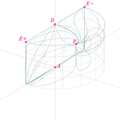
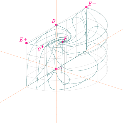
Figure 1: Phase-space trajectories for model $\mathcal{A}$. The left plot shows the stable node G, with $\lambda=1.2$ and $\alpha=10^{-3}$. The right plot shows the stable focus F with $\lambda=2.3$ and $\alpha=10^{-3}$

This model depicts an evolution of the universe in good agreement with the observations for certain values of the parameters $\lambda,\alpha$. Saddle point A corresponds to the standard matter dominated universe with $a(t)\propto t^{2/3}$; its instability allows for the existence of trajectories escaping from it and ending at an attractor, which exists for adequate values of the parameters. However, the attractor (or late time stage of the universe) will only represent an accelerated scenario for a flat enough potential, specifically when $\lambda^{2}<2$. In this case the attractor is completely dark energy dominated, point G. If the potential is not flat enough, the attractor, point F, is a scaling solution, in which the fraction of dark energy is the dominant one.

One way to understand this behaviour is by looking at the relative strength of the coupling, $f$, in the CDM balance equation,

$$f:=\frac{|Q|}{H\rho_{c}}\,.$$ (27)

In the matter era, $H^{2}={\rho_{c}}/{3},$ we have

$$f\sim\rho_{\phi}^{2}/\rho_{c}^{3/2},$$ (28)

which is decreasing into the past. Thus the coupling is weaker in the past and this allows a near-standard matter era. It is important to note that the dynamical behaviour of the standard matter point A and the accelerated critical solution G does not depend on the sign of the coupling parameter $\alpha$.

III.2 Model $\mathcal{B}$: coupling $Q=\frac{\beta}{H_{0}}\rho_{c}^{2}$

The autonomous system is

$$x^{\prime} =-3x+\lambda\frac{\sqrt{6}}{2}\,y^{2}+\frac{3}{2}x(1+x^{2}-y^{2})+\beta\,\frac{3(1-z)(1-x^{2}-y^{2})^{2}}{2xz}\,,$$ (29)

$$y^{\prime} =-\lambda\frac{\sqrt{6}}{2}\,xy+\frac{3}{2}y(1+x^{2}-y^{2})\,,$$ (30)

$$z^{\prime} =\frac{3}{2}z(1-z)(1+x^{2}-y^{2})\,.$$ (31)

The critical points and their stability properties are summarized in Tables 3 and 4 respectively.

Point	$x_{*}$	$y_{*}$	$z_{*}$	Eigenvalues	$w_{tot}$
B±	$\pm 1$	$0$	$0$	$3\,,3\,,3\mp\sqrt{\frac{3}{2}}\lambda$	1
C	$\frac{\lambda}{\sqrt{6}}$	$\sqrt{1-\frac{\lambda^{2}}{6}}$	0	$\frac{\lambda^{2}}{2}\,,\frac{\lambda^{2}}{2}-3\,,\lambda^{2}-3$	$\frac{\lambda^{2}}{3}-1$
D	$0$	$0$	$1$	$-\frac{3}{2}\,,-\frac{3}{2}\,,\frac{3}{2}$	0
E±	$\pm 1$	$0$	$1$	$-3\,,3\,,3\mp\sqrt{\frac{3}{2}}\lambda$	1
F	$\sqrt{\frac{3}{2}}\frac{1}{\lambda}$	$\sqrt{\frac{3}{2}}\frac{1}{\lambda}$	1	$-\frac{3}{2}\,,-\frac{3}{4\lambda}(\lambda\pm\sqrt{24-7\lambda^{2}})$	0
G	$\frac{\lambda}{\sqrt{6}}$	$\sqrt{1-\frac{\lambda^{2}}{6}}$	1	$-\frac{\lambda^{2}}{2}\,,-3+\frac{\lambda^{2}}{2}\,,-3+\lambda^{2}$	$\frac{\lambda^{2}}{3}-1$

Table 3: Critical points and associated eigenvalues for coupling model $\mathcal{B}$.

Point	Stable?	$\Omega_{\phi}$	$w_{T}$	Acceleration?	Existence
B+	Saddle node for $\lambda>\sqrt{6}$	1	1	No	$\forall\,\lambda,\,\beta$
	Unstable node for $\lambda<\sqrt{6}$
B-	Unstable node for $\lambda>-\sqrt{6}$	1	1	No	$\forall\,\lambda,\,\beta$
	Saddle node for $\lambda<-\sqrt{6}$
C	Saddle node	1	$\frac{\lambda^{2}}{3}-1$	$\lambda^{2}<2$	$\lambda^{2}<6$
D	Saddle node	0	0	No	$\forall\,\lambda,\,\beta$
E±	Saddle node	1	1	No	$\forall\,\lambda,\,\beta$
F	Stable focus for $\lambda^{2}>\frac{24}{7}$	$\frac{3}{\lambda^{2}}$	0	No	$\lambda^{2}>3$
	Stable node for $3<\lambda^{2}<\frac{24}{7}$
G	Saddle node for $\lambda^{2}>3$	1	$\frac{\lambda^{2}}{3}-1$	$\lambda^{2}<2$	$\lambda^{2}<6$
	Stable node for $\lambda^{2}<3$

Table 4: The properties of the critical points for model $\mathcal{B}$.

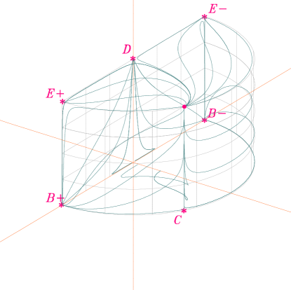
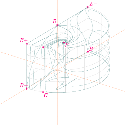
Figure 2: Phase-space trajectories for model $\mathcal{B}$. The left plot shows the stable node G, with $\lambda=1.2$ and $\beta=10^{-3}$. The right plot shows the stable focus F with $\lambda=2.3$ and $\beta=10^{-3}$.

This model does not have a unstable standard matter solution, so it cannot depict an evolution from an early dust-like scenario. However, there is a solution in which the dark energy can mimic such behaviour for $\lambda^{2}=3$. This is saddle point C, but the $\lambda$ value allowing for that point to act like matter prevents the existence of an accelerated solution at late times. Regarding the late-time attractor we meet again the same situation as before, a scaling but dark energy dominated non accelerated solutions for excessively shallow potentials, and an accelerated completely dark energy dominated scenario in the opposite case. The relative strength of the coupling Eq. (27) for this model is

$$f\sim H\,,$$ (32)

and is increasing to the past. Since the coupling gets stronger at early times we cannot get a standard matter era. The direction of the energy exchange does not affect this conclusion.

III.3 Model $\mathcal{C}$: coupling $Q=\frac{\gamma}{H_{0}}\rho_{c}\rho_{\varphi}$

In this case,

$$x^{\prime} =-3x+\lambda\frac{\sqrt{6}}{2}\,y^{2}+\frac{3}{2}x(1+x^{2}-y^{2})+\gamma\,\frac{3(1-z)(1-x^{2}-y^{2})(x^{2}+y^{2})}{2xz}\,,$$ (33)

$$y^{\prime} =-\lambda\frac{\sqrt{6}}{2}\,xy+\frac{3}{2}y(1+x^{2}-y^{2})\,,$$ (34)

$$z^{\prime} =\frac{3}{2}z(1-z)(1+x^{2}-y^{2})\,,$$ (35)

and we summarize the critical points and stability in Tables 5 and 6.

Point	$x_{*}$	$y_{*}$	$z_{*}$	Eigenvalues	$w_{tot}$
A	$0$	$0$	$0$	$\frac{3}{2}\,,\frac{3}{2}\,,\operatorname{{\mathrm{s}gn}}(\gamma)\infty$	0
B±	$\pm 1$	0	0	$3\,,3\mp\sqrt{\frac{3}{2}}\lambda\,,-\operatorname{{\mathrm{s}gn}}(\gamma)\infty$	1
C	$\frac{\lambda}{\sqrt{6}}$	$\sqrt{1-\frac{\lambda^{2}}{6}}$	0	$\frac{\lambda^{2}}{2}\,,\frac{\lambda^{2}}{2}-3\,,-\operatorname{{\mathrm{s}gn}}(\gamma)\infty$	1
D	0	0	1	$-\frac{3}{2}\,,-\frac{3}{2}\,,\frac{3}{2}$	0
E±	$\pm 1$	0	1	$-3\,,3\,,3\mp\sqrt{\frac{3}{2}}\lambda$	1
F	$\sqrt{\frac{3}{2}}\frac{1}{\lambda}$	$\sqrt{\frac{3}{2}}\frac{1}{\lambda}$	1	$-\frac{3}{2}\,,-\frac{3}{4\lambda}(\lambda\pm\sqrt{24-7\lambda^{2}})$	0
G	$\frac{\lambda}{\sqrt{6}}$	$\sqrt{1-\frac{\lambda^{2}}{6}}$	1	$-\frac{\lambda^{2}}{2}\,,-3+\frac{\lambda^{2}}{2}\,,-3+\lambda^{2}$	$\frac{\lambda^{2}}{2}-1$

Table 5: Critical points and associated eigenvalues for coupling model $\mathcal{C}$.

Point	Stable?	$\Omega_{\phi}$	$w_{T}$	Acceleration?	Existence
A	Unstable node for $\gamma>0$	0	0	No	$\forall\,\lambda,\,\gamma$
	Saddle node for $\gamma<0$
B+	Unstable node for$\lambda<\sqrt{6}$ and $\gamma<0$	1	1	No	$\forall\,\lambda,\,\gamma$
	Saddle otherwise
B-	Unstable node for $\lambda>-\sqrt{6}$ and $\gamma<0$	1	1	No	$\forall\,\lambda,\,\gamma$
	Saddle otherwise
C	Saddle node	1	$\frac{\lambda^{2}}{3}-1$	$\lambda^{2}<2$	$\lambda^{2}<6$
D	Saddle node	0	0	No	$\forall\,\lambda,\,\beta$
E±	Saddle node	1	1	No	$\forall\,\lambda,\,\beta$
F	Stable focus for $\lambda^{2}>\frac{24}{7}$	$\frac{3}{\lambda^{2}}$	0	No	$\lambda^{2}>3$
	Stable node for $3<\lambda^{2}<\frac{24}{7}$
G	Saddle node for $\lambda^{2}>3$	1	$\frac{\lambda^{2}}{3}-1$	$\lambda^{2}<2$	$\lambda^{2}<6$
	Stable node for $\lambda^{2}<3$

Table 6: The properties of the critical points for model $\mathcal{C}$.

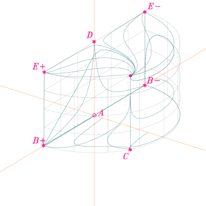
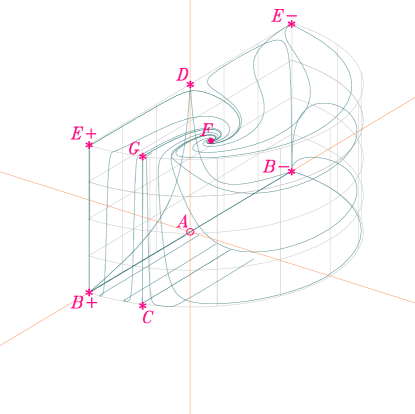
Figure 3: Phase-space trajectories for model $\mathcal{C}$. The left plot shows the stable node G, with $\lambda=1.2$ and $\gamma=10^{-3}$. The right plot shows the stable focus F with $\lambda=2.3$ and $\gamma=10^{-3}$.

This model has interesting properties. First of all, a standard matter represented by the unstable point $A$ exists. In particular when $\gamma>0$, the instability of the point is generic, as it is occurs in all directions; whereas for $\gamma<0$ the point becomes a saddle. Secondly, an accelerated attractor exists for adequate values of the parameters. The two possible late-time attractors as in the other two cases are found again, and the same conditions as in those cases operate in connection with the kinematical features of the scenario they represent, if $\lambda$ is not small enough, acceleration will not be possible and in addition dark energy will not dominate completely.

The coupling strength for this model, Eq. (27) is decreasing into the past as

$$f\sim{\rho_{\phi}}^{2}/\rho_{c}^{1/2}\,.$$ (36)

III.4 Superposition of couplings

When we combine the different coupling models together, we expect only those critical points to be present which are critical points of each individual model. Since we want to describe the evolution of a universe that includes a standard matter era and evolves towards a stable accelerating solution, we must choose the combination of models $\mathcal{A}$ and $\mathcal{C}$, since those are the ones that allow for a standard matter era. Therefore we consider the composite model defined by the coupling

$$Q=\frac{\alpha}{H_{0}}\rho_{\varphi}^{2}+\frac{\gamma}{H_{0}}\rho_{c}\rho_{\varphi}\,.$$ (37)

We note that the two couplings are decoupled in the sense that there are no cross coupling terms in the dynamical system.

The resulting system of autonomous differential equations reads

$$x^{\prime} =-3x+\lambda\frac{\sqrt{6}}{2}\,y^{2}+\frac{3}{2}x(1+x^{2}-y^{2})+\alpha\,\frac{3(1-z)(x^{2}+y^{2})^{2}}{2xz}+\gamma\,\frac{3(1-z)(1-x^{2}-y^{2})(x^{2}+y^{2})}{2xz}\,,$$ (38)

$$y^{\prime} =-\lambda\frac{\sqrt{6}}{2}\,xy+\frac{3}{2}y(1+x^{2}-y^{2})\,,$$ (39)

$$z^{\prime} =\frac{3}{2}z(1-z)(1+x^{2}-y^{2})\,.$$ (40)

The critical points and their stability are listed in Tables 7 and 8.

Point	$x_{*}$	$y_{*}$	$z_{*}$	Eigenvalues	$w_{tot}$
A	$0$	$0$	$0$	sgn$(\gamma)\infty\,,\frac{3}{2}\,,\frac{3}{2}$	0
D	$0$	$0$	$1$	$-\frac{3}{2}\,,-\frac{3}{2}\,,\frac{3}{2}$	0
$\mathrm{E}_{\pm}$	$\pm 1$	$0$	$1$	$-3\,,3\,,3\mp\sqrt{\frac{3}{2}}\lambda$	1
F	$\frac{1}{\lambda}\sqrt{\frac{3}{2}}$	$\frac{1}{\lambda}\sqrt{\frac{3}{2}}$	$1$	$-\frac{3}{2}\,,-\frac{3}{4\lambda}(\lambda\pm\sqrt{24-7\lambda^{2}})$	0
G	$\frac{\lambda}{\sqrt{6}}$	$\sqrt{1-\frac{\lambda^{2}}{6}}$	$1$	$-\frac{\lambda^{2}}{2}\,,-3+\frac{\lambda^{2}}{2}\,,\lambda^{2}-3$	$\frac{\lambda^{2}}{2}-1$

Table 7: Critical points and associated eigenvalues for the superposition of couplings for model $\mathcal{A}$ and model $\mathcal{C}$.

Point	Stable?	$\Omega_{\phi}$	$w_{T}$	Acceleration?	Existence
A	Unstable node for $\gamma>0$	0	0	No	$\forall\,\lambda,\,\alpha,\,\beta,\gamma$
	Saddle node for $\gamma<0$
D	Saddle node	0	0	No	$\forall\,\lambda,\,\alpha,\,\beta,\gamma$
E±	Saddle node	1	1	No	$\forall\,\lambda,\,\alpha,\,\beta,\,\gamma$
F	Stable focus for $\lambda^{2}>\frac{24}{7}$	$\frac{3}{\lambda^{2}}$	0	No	$\lambda^{2}>3$
	Stable node for $3<\lambda^{2}<\frac{24}{7}$
G	Saddle node for $\lambda^{2}>3$	1	$\frac{\lambda^{2}}{3}-1$	$\lambda^{2}<2$	$\lambda^{2}<6$
	Stable node for $\lambda^{2}<3$

Table 8: The properties of the critical points for the superposition of couplings.

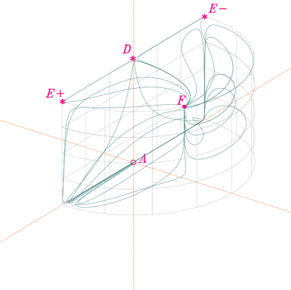
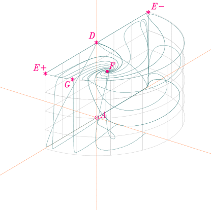
Figure 4: Phase-space trajectories for the superposition of couplings. The left plot shows the stable node G, with $\lambda=1.2$ and $\alpha=2\gamma=2\times 10^{-3}$. The right plot shows the stable focus F with $\lambda=2.3$ and $\alpha=2\gamma=2\times 10^{-3}$.

Points A and D correspond to the standard matter era and point G is the accelerated attractor for $\lambda^{2}<2$.

IV Conclusions

We have made a comprehensive analysis of the background dynamics for a new class of models with quadratic dark sector coupling, which are a simple physically-motivated generalization of the linear coupling couplings with constant rates of energy transfer, given in Boehmer et al. (2008); Valiviita et al. (2008); Caldera-Cabral et al. (2009b). The two species which interact are dark matter and quintessence with an exponential self-interaction potential.

Of the three different terms in the general quadratic coupling, we found that the term $Q=\mathcal{B}\rho_{c}^{2}$ leads to a universe without a standard matter era, whereas the other two terms, $Q=\mathcal{A}\rho_{\varphi}^{2}$ and $Q=\mathcal{C}\rho_{c}\rho_{\varphi}^{2}$, do admit a standard matter era and an evolution that connects this to a late-time attractor. This attractor is accelerated provide the potential is flat enough. The models we have analysed provide us with the following partial answers. These features are valid for both signs of $\mathcal{A}$ or $\mathcal{C}$, i.e the evolution is not affected by the direction of the energy transfer. But in the $\mathcal{C}>0$ case the instability of the matter era is more generic; so there is in a way more room for a transition from the matter era to the accelerated attractor. In other words, in theses case there are less restrictions on the initial conditions for this desired transition between asymptotic states to occur.

The critical point for late-time acceleration, G, is not a scaling solution, since

$$\Omega_{c*}=0\,,\qquad\Omega_{\varphi*}=1\,.$$ (41)

This is similar to the asymptotic behaviour of the standard $\Lambda$CDM model. Thus the quadratic models do not produce a constant non-zero and finite ratio $\Omega_{c*}/\Omega_{\phi*}$, and therefore do not address the coincidence problem in this sense. The linear coupling $Q=\Gamma\rho_{c}$ leads the same critical point G; this accelerated solution is an attractor when $\Gamma>0$, i.e when dark matter is decaying into dark energy.

The quadratic models which admit a viable background evolution can be compared to observations in order to constrain the parameters $\alpha$ and $\gamma$. This will require an investigation of the cosmological perturbations in these models.