The Planck Satellite: Status & Perspectives

Planck was successfully launched on May 14th, 2009, from the Kourou space port, in French Guyana. After recalling the objectives that we set out - back in 1996 - to fulfill with this project, I recall some of the technological breakthroughs which needed to be made and report on the exciting scientific outlook of the project in light of the knowledge we now have of the actual performances of the two on-board instruments. I also include one of our more recent results even though it was not yet available at the time of the conference.

The measurement goals of Planck may be stated rather simply: to build an experiment able to perform the “ultimate” measurement of the primary CMB temperature anisotropies, which requires:

• full sky coverage and a good enough angular resolution in order to completely mine all scales at which the Cosmic Microwave background (CMB) primary anisotropies contain information (${\lower 2.15277pt\hbox{$\;\buildrel>\over{\sim}\;$}}5$ minutes of arc)

• a final sensitivity essentially limited by the ability to remove the astrophysical foregrounds, implying a large frequency coverage from 30 GHz to 1 THz (provided by the two instruments: HFI and LFI), with sensitivity at each of the 9 survey frequencies in line with the role of each map in determining the CMB properties .

For the measurement of the polarisation of the CMB anisotropies, Planck goal was “only” to get the best polarisation performances with the technology available at the design time

This is on these simple but ambitious goals and the proposed way of reaching them that, after 3 years of preparatory work, the project was selected by the European Space Agency (ESA), as the $3^{rd}$ Medium size mission of its Horizon 2000+ program. This selection occurred in march 1996, i.e. contemporaneously with that of WMAP by NASA, which rather proposed reaching earlier less ambitious goals with already existing technology.

Table 1: Summary of Planck performance goals for the required 14 months of routine operations, which allows nearly all detectors to map the entire sky twice. Requirements on sensitivity are simply two times worse than the stated goals. Central band frequencies, $\nu$, are in Gigahertz, the FWHM angular sizes are in arc minute, and the (sky-averaged) sensitivities $c^{X}_{noise}$, with $X=T,Q$ or $U$, are expressed in $\mu\mathrm{K.deg}$; this number indicates the rms detector noise, expressed as a equivalent temperature fluctuation in $\mu\mathrm{K}$, whcih is expected once it is averaged in a pixel of 1 degree of linear size).

	LFI goals			HFI goals
$\nu$ [GHz]	30	44	70	100	143	217	353	545	857
FWHM [arcmin]	33	24	14	9.5	7.1	5.0	5.0	5.0	5.0
$c^{T}_{noise}$ [$\mu\mathrm{K.deg}$]	3.0	3.0	3.0	1.1	1.4	2.2	6.8	-	-
$c^{QorU}_{noise}$ [$\mu\mathrm{K.deg}$]	4.5	4.6	4.6	1.8	1.4	2.4	7.3

Table 1 summarises the main performance goals of Planck, expressed for instance as the average detector noise within a square patch of 1 degree of linear size, $c_{noise}$, for the 14 months baseline duration of the mission, which would allow covering twice all the sky by nearly all the detectors. It is interesting to note that if we take the noise performance figure for the average of the central CMB frequencies (the 100-143-217 GHz HFI  channels, assuming all the other channels are devoted to foregrounds removal), one finds $0.5\ \mathrm{\mu K.deg}$ in temperature and $1\ \mathrm{\mu K.deg}$ for the Q & U Stokes parameters. The magnitude of this step forward, if achieved, may be judged by comparing with the WMAP sensitivity which is given in Table 2. The aggregate sensitivity of the WMAP 60 & 90 GHz channels is $\sim 10.8\ \mathrm{\mu K.deg}$ in a year, which would imply about $(10.8/.5)^{2}\sim$ 460 years of operations to reach the baseline Planck sensitivity. In other words, the error bars from noise in the angular power spectrum should be at least hundred times smaller for Planck than for WMAP(with an even larger difference at smaller scales which will be much better known from Planck  thanks to the twice higher angular resolution of HFI).

Table 2: Summary of WMAP in-flight performance per full year of operations. Same units than in Table 1.

WMAP (in flight)
$\nu$ [GHz]	23	33	41	61	94
FWHM [arc min]	49.2	37.2	29.4	19.8	12.6
$c^{T}_{noise}$ [$\mu\mathrm{K.deg}$]	12.6	12.9	13.3	15.6	15.0

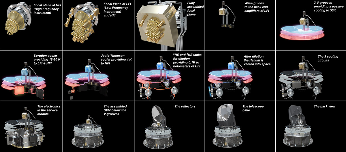
Figure 1: Planck build-up from the inside out. Going from left to right, one sees on the top row (t1) the HFI instrument with its 52 detector horns poking out of it’s outer shell at 4 K. (t2) HFI is surrounded by the 11 larger horns from LFI. HFI and LFI together form (t3) the focal plane assembly from which (t4) the electrical signal departs (though a bunch of wave guides for the LFI and a harness of wires for HFI) to connect to the warm electronics parts of the detection chain which are located within the service module at $\sim$ 300 K. (t5) The (top) cold and warm (bottom) parts are separated by three thermally isolating V-grooves which allow radiating to space heat from the spacecraft sideways and quite efficiently. The third (top) V-grooves operating temperature is about 40 K. On the middle row, one sees (m1) the beds of the sorption cooler and it’s piping around the V-groove, bringing the overall focal-plane structure to LFI’s operational temperature of $\sim 18$  K. (m2) The back-to-back (to damp the first harmonics of the vibrations) compressors of the 4 K cooler allow bringing HFI outer shell to 4 K, while (m3) isotopes from the He3 tank and the three He4 tanks are brought to the mixing pipes within HFI to cool filters (within the horns) to 1.6 K and the bolometer plate to 0.1 K, before (m4) being released to space. (m5) The passive cooling and the three active stage constitute this complex but powerful cooling chain in space. On the last bottom row, one can also see (b1) some of the electronic boxes in the service module (SVM) which in addition to the warm part of the electronic and cooling chains also contain all “services” needed for transmitting data, reconstructing the spacecraft attitude, powering the whole satellite… The bottom of the SVM is covered with solar panels, while supporting struts begin on its top which allows (b3) positioning the secondary and primary reflectors. The top part is surrounded by a large baffle to shield at best the focal plane from stray-light. The back view (b5) allows distinguishing in the back the supporting structure of the primary mirror, and the wave guides from LFI. The spin axis of Planck (vertical on these plots) is meant to be close to the sun-earth line, with the solar panel near perpendicular to that line and the rotation of the line-of-sight (at 1 rpm) causing the detectors to survey circles on the sky with an opening angle around 85 degrees. Copyright ESA.

We proposed to achieve the ambitious sensitivity goals of Planck with a small number of detectors, limited principally by the photon noise of the background (for the CMB ones), in each frequency band. This implied to achieve several technological feats never achieved in space before (see in particular Lamarre et al. 2003, in New Astronomy Reviews, 47, pp. 1017):

• sensitive & fast bolometers with a Noise Equivalent Power $<2\times 10^{-17}\ \mathrm{W/Hz}^{1/2}$ and time constants typically smaller than about 5 milliseconds (which thus requires cooling them down to $\sim 100$ mK, and build them with a very low heat capacity & charged particles sensitivity)

• total power read out electronics with very low noise, $<6\ \mathrm{nV/Hz}^{1/2}$ from 10 mHz (1 rpm) to 100 Hz (i.e. from the largest to the smallest angular scales to measure at the Planck scanning speed)

• excellent temperature stability, from 10 mHz to 100 Hz (cf. Lamarre et al. 04), such that the induced variation be a small fraction of the detector temporal noise:

  • better than $10\ \mathrm{\mu K/Hz}^{1/2}$ for the 4K box (assuming 30% emissivity)

  • better than $30\ \mathrm{\mu K/Hz}^{1/2}$ on the 1.6K filter plate (assuming a 20% emissivity)

  • better than $20\ \mathrm{nK/Hz}^{1/2}$ for the detector plate (a damping factor $\sim 5000$ needed)

• very low noise HEMT amplifiers (therefore cooled to 20 K) & very stable cold reference loads (at 4 K)

In addition, Planck requires:

• a low emissivity telescope with very low side lobes (i.e. strongly under-illuminated)

• no windows, and minimum warm surfaces between the detectors and the telescope

• a quite complex cryogenic cooling chain (cf. figure 1) which begins by reaching $\sim 40K$ via passive cooling, by radiating about 2 Watts to space, followed by three active stages, at 20 K, 4 K, and 0.1 K:

  • 20 K for the LFI, with a large cooling power, $\sim 0.7$ Watts (provided by $H_{2}$ Joule-Thomson sorption pumps developed by JPL, USA)

  • 4 K, 1.6 K and 100 mK for the HFI (the 15 milli-Watts cooling power at 4K is provided by mechanical pumps provided by the RAL, UK, in order to perform a Joule-Thomson expansion of He; the 1.6K stage has a pre-cooling power of about 0.5 milli-Watts, thanks to another Joule-Thomson expansion, while the final dilution fridge of He³ & He⁴, from a French collaboration between Air Liquide, the CRTBT, can deal with 0.2 micro-Watts at 0.1 K).

  • a thermal architecture optimised to damp thermal fluctuations (active+passive)

Furthermore, a tight control of vibrations is needed, in particular since the dilution cooler does not tolerate micro-vibrations at sub-mg level. And as little as $7\times 10^{10}$ He atoms accumulated on the dilution heat exchanger (an He pressure typically at the $1\times 10^{-10}$ mb level) would be too much.

These top-level design goals have now been turned into real instruments, which went through several qualification models. Before delivering the actual flight model of both instruments to industry for integration with the satellite, both instrumental consortia organised extensive calibrations campaigns starting at the individual components levels, then at the sub-systems levels (e.g. individual photometric pixels), then at instrument level. For HFI, the detector-level tests were done mainly at JPL in the USA, and the pixel level tests were performed in Cardiff in the UK, while the flight instrument calibration was performed at the Institut d’Astrophysique Spatiale in Orsay, France from April till the end of July 2006. During that period, we obtained in particular 19 days of scientific data at normal operating conditions. We could then confirm that HFI satisfies all our requirements, and for the most part actually reaches or exceeds the more ambitious design goals, in particular concerning the sensitivity, and speed of the bolometers, the very low noise of the read out electronics and the overall thermal stability. In addition, the total optical efficiency has been verified to be satisfactory, optical cross-talk appears negligible, as well as the Current cross-talk and the cross-talk in intensity is weak. Main beams are well-defined and are quite well described by the models, polarisation measurements confirm expectations, etc. The LFI instrument also went through detailed testing around the same time and it does reach most of its ambitious requirements.

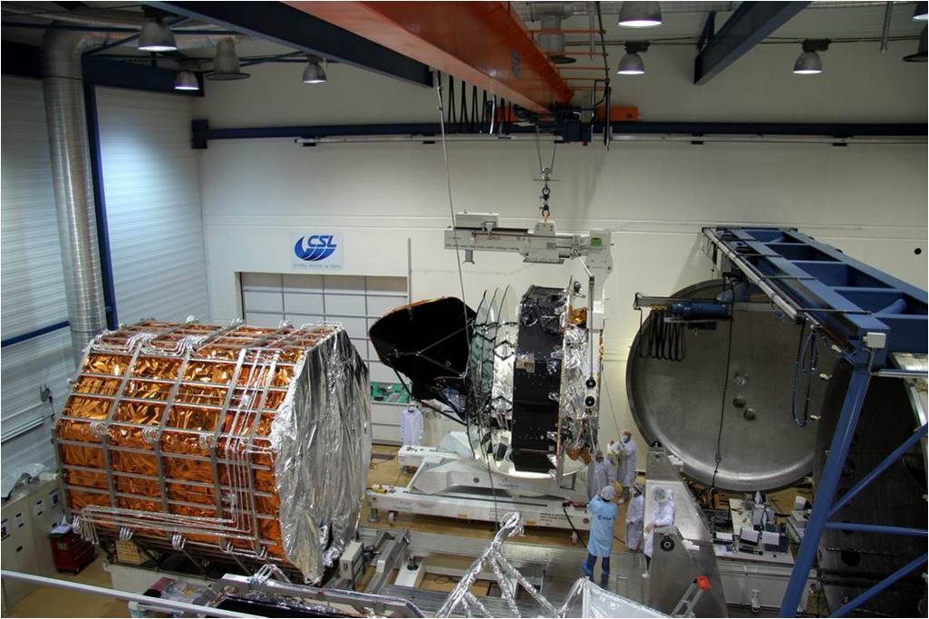
Figure 2: Planck on May 2008, hanging outside the vacuum cryogenic chamber at CSL before completing it’s first and last full thermal vacuum test. Copyright ESA.

The integration of the LFI and HFI instruments was performed at Thales premises in Cannes in November 2006 and within a year, by December 2007, the full satellite was ready for vibration testing. Planck was then flown from Cannes to ESA’s ESTEC centre (in Noordwijk, Holland) where among other things it went through load balancing on April 7th, before travelling again to the “Centre Spatial de Liéges” (CSL) in april 2008. Figure 2 is a picture of Planck hanging outside the vacuum cryogenic chamber at CSL, before the start of the first (and last) full thermal test with all elements of the cryogenic chain present and operating. This ultimate system-level (ground) test demonstrated in particular the following:

• the dilution system can work with the minimal Helium 3 and 4 flux, which should allow 30 months of survey duration (nominal duration being 14 months!)

• the extremely demanding temperature stability required (at 1/5 of the detection noise) has been verified

• bolometers sensitivities in flight conditions are indeed centered around the goal, as shown in figure 3.

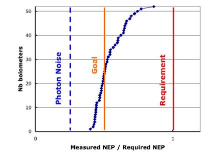
Figure 3: Measured values of the Noise Equivalent Power of HFI detectors during the ground test in flight conditions at CSL on May 2008. One sees that the median value is at the goal level.

Planck was then shipped to Kourou, and after a few more nerve –wracking delays, we finally lost sight of Planck for ever (when it was covered by the SYLDA support system on the top of which laid Herschel for a joint launch). Launch was on May 14th, and it was essentially perfect. After separating from Herschel, Planck was set in rotation and started its to the L2 Lagrange point of the sun-earth system, at 1.5 million kilometres away from earth, i.e. about 1% further away from the sun than the earth. The final injection in the L2 orbit was at the end of June, shortly after the end of the Blois meeting (see figure 4-a), at the same time than the cooling sequence ended successfully. Indeed, figure 4-b shows how the various thermal stages reached their operating temperature, cooling of coarse from the outside-in, and closely following the predicted pattern.

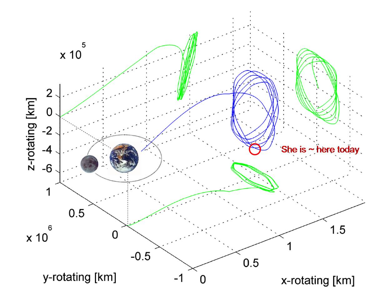
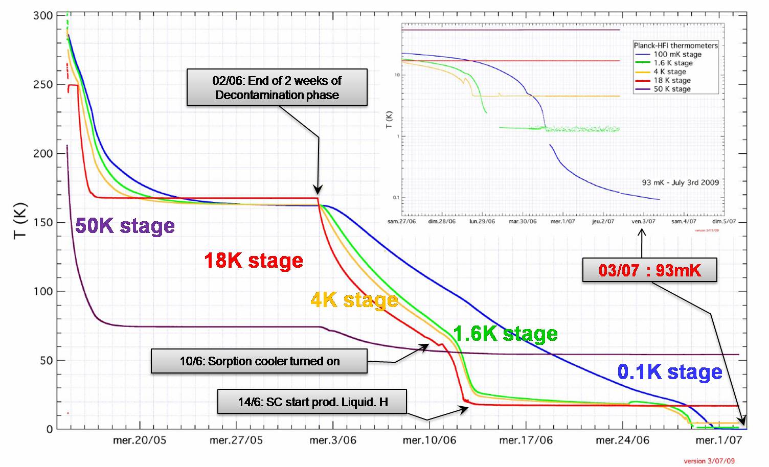
Figure 4: a) Spacecraft trajectory to and on the L2 orbit. b) Cooling sequence of Planck, showing the various stages reaching in turn their operational temperature, till the dilution plate actually reached 93 mK on July 3rd. Credit ESA and HFI consortium

Once at L2, a calibration and performance verification phase was conducted till mid-august, to insure that all system are working properly and that instrumental parameters are all set at best. From August 13th to 27th, we conducted a “First Light Survey” (FLS) in normal operational mode for an ultimate verification of parameters and of the long-term stability of the experiment. We found the data quality to be excellent, and the Data processing Centre pipelines could be operated as hoped to produce the first images. Figure 5 (extracted from the Press release we made on September 17th) illustrates the FLS coverage by showing an image generated from the data acquired from a single 100GHz detector of HFI superimposed to an image of the optical sky by Axel Mellinger. We also released (see the press release in English at ESA’s site http://sci.esa.int/science-e/www/object/index.cfm?fobjectid=45543 and in French at http://public.planck.fr/actualiteFLS.php) a comparison of a high latitude field whose emission ought to be dominated by the CMB (shown by a small white square in the figure) as observed by an HFI and LFI detector. They demonstrate an excellent similarity while the two instruments are using quite different technologies. Nine images at all the frequencies covered by Planck of a Galaxy crossing area (indicated by the large white square of the figure) provide visual evidence to the richness of the dataset that Planck shall deliver, allowing very broad scientific studies outreaching its primary cosmological goals. Indeed an important part of Planck long term legacy will be the unique set of maps of the millimetric and sub-millimetric polarised full sky.

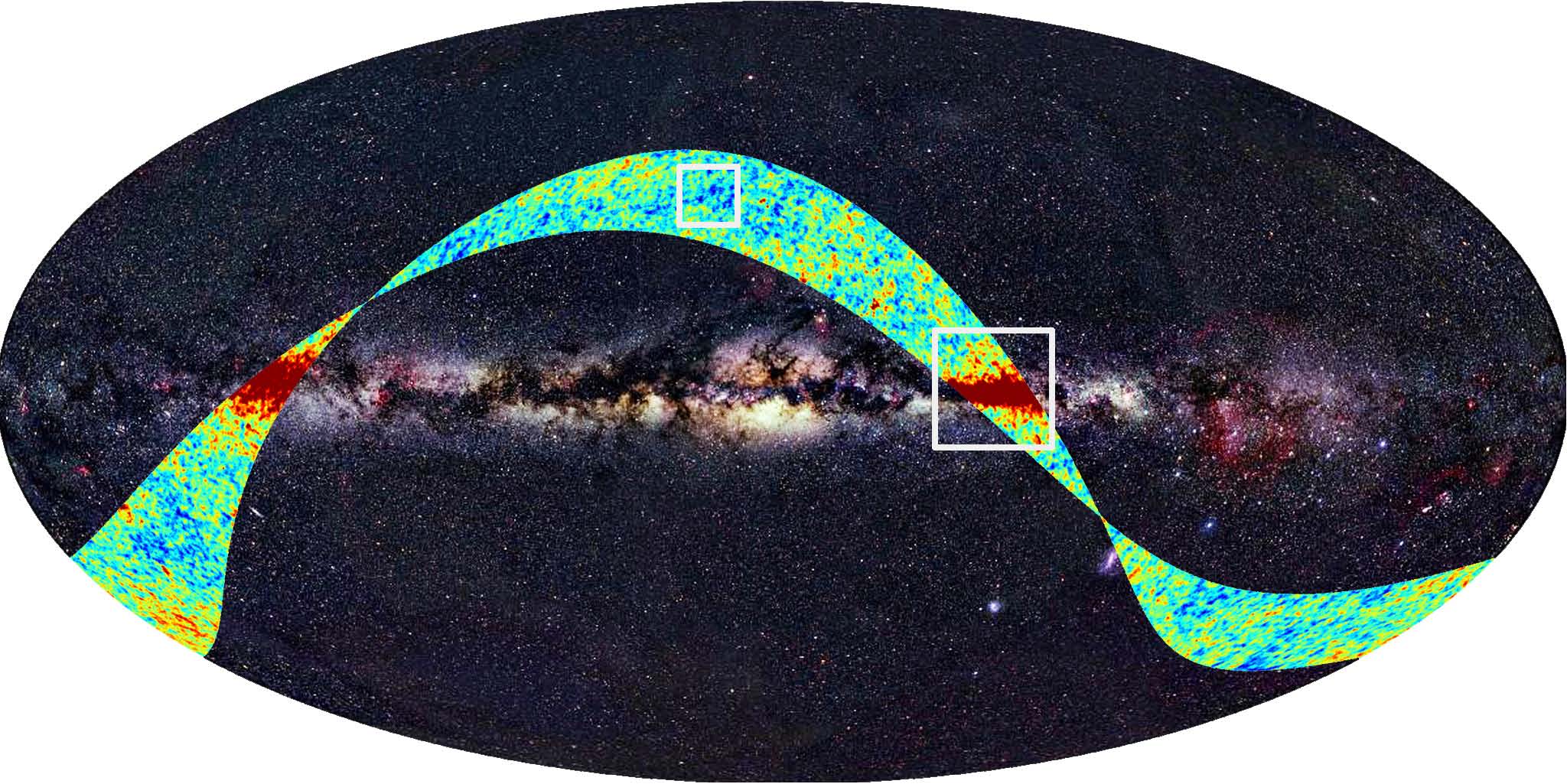
Figure 5: Sky coverage during Planck First Light Survey (FLS). Planck measures a ring of about 1 degree per day (for a full rotation around the sun in a year), yielding this $\sim 15$ degree strip during the two weeks of the FLS. The detector image shown in Galactic coordinates is superimposed to a background image where the Galactic plane is clearly visible. Credit ESA and HFI & LFI consortia.

With the success of the FLS, the normal survey operations have now started. We should therefore be in a position to deliver in December 2010, as planned, an “Early Release Point Source Catalogue” based on a rapid analysis of the first coverage of the sky which will be issued in time to allow the astrophysical community at large to propose follow-ups by Herschel during its expected cryogenic life. A first public release based on the data from the nominal 14 months mission is slated for december 2012. The release should contain the clean calibrated time-ordered data of each detector, the nine full sky maps at the six frequencies covered by HFI and the three ones by LFI, possibly supplemented by polarisation maps, as well as maps of identified astrophysical components (CMB, Galactic Emissions, Extragalactic sources catalogue), some ancillary information (e.g. on beams, spectral transmission, etc), accompanied by about 50 scientific papers describing the mission, how the “products” were obtained, validated, and the results of a first pass of scientific exploitation by the Planck collaboration itself, encompassing in particular the implications of the measured statistical properties of the CMB. Our anticipation from the measured Helium consumption in flight is that the mission duration will exceed the nominal duration of 14 months, and we plan a further release, about a year later on the basis of the extra data which might allow covering as much as five times in total the entire sky. In addition to an improved sensitivity, this extra duration will foremost allow greater data redundancy and therefore a tighter control of all systematic effect which can be searched for with a longer baseline. This should allow us detecting the gravitational wave stochastic background predicted in one interesting class of inflationary models, providing the long thought after “smoking gun” of inflation, or otherwise put meaningful constraints on the viable inflation models remaining.

In conclusion, Planck is now in normal operation & performances are as expected or better.
This gives us confidence that the scientific program of Planck can be carried through as anticipated. The dataset should in particular allow addressing many key cosmological questions, including the existence of a primordial gravitational wave background, or that of highly revealing deviations from the current minimal model, where the primordial fluctuation can be purely Gaussian, adiabatic, scale-free, in a strictly flat spatial geometry with a dark energy component describable as a pure cosmological constant, and (cosmologically) negligible neutrinos masses.

A rather complete overview of the scientific Program of Planck can be found in the so-called “Blue Book” which was issued in 2004. It can be downloaded from
http://www.planck.fr/IMG/pdf/Planck_book.pdf.
In addition, we submitted a series of pre-launch papers (all with a title starting with “Planck pre-launch status:”) giving many details of the design and tests of the mission, the instruments, and some of their components.