The 400d Galaxy Cluster Survey Weak Lensing Programme:
I: MMT/Megacam Analysis of CL0030+2618 at $z\!=\!0.50$

Abstract

Context. Cosmological structure formation offers insights on all of the universe’s components: baryonic matter, dark matter, and, notably, dark energy. The mass function of galaxy clusters at high redshifts is a particularly useful probe to learn about the history of structure formation and constrain cosmological parameters.

Aims. We aim at deriving reliable masses for a high-redshift, high-luminosity sample of clusters of galaxies selected from the 400d survey of X-ray selected clusters. Weak gravitational lensing allows a comparison of the mass estimates derived from X-rays, forming an independent test. Here, we will focus on a particular object, CL0030+2618 at $z\!=\!0.50$.

Methods. Using deep imaging in three passbands with the Megacam instrument at MMT, we show that Megacam is well-suited for measuring gravitational shear, i.e. the shapes of faint galaxies. A catalogue of background galaxies is constructed by analysing photometric properties of galaxies in the $g^{\prime}r^{\prime}i^{\prime}$ bands.

Results. We detect the weak lensing signal of CL0030+2618 at $5.8\sigma$ significance, using the aperture mass technique. Furthermore, we find significant tangential alignment of galaxies out to $\sim\!10\arcmin$ or $>\!2\leavevmode\nobreak\ r_{200}$ distance from the cluster centre. The weak lensing centre of CL0030+2618 agrees with several X-ray measurements and the position of the brightest cluster galaxy. Finally, we infer a weak lensing virial mass of $M_{200}\!=\!7.2^{+3.6+2.3}_{-2.9-2.5}\times 10^{14}\mathrm{M}_{\sun}$ for CL0030+2618.

Conclusions. Despite complications by a tentative foreground galaxy group in the line of sight, the X-ray and weak lensing estimates for CL0030+2618 are in remarkable agreement.

1 Introduction

The mass function $n(M,z)$ of galaxy clusters is a sensitive probe to both cosmic expansion and evolution of structure by gravitational collapse (cf. e.g., Rosati et al. 2002; Voit 2005; Schuecker 2005). Therefore, mass functions derived from statistically well-understood cluster samples can be and are frequently used to determine cosmological parameters like $\Omega_{\mathrm{m}}$, the total matter density of the universe in terms of the critical density, and $\sigma_{8}$, the dispersion of the matter density contrast. In addition, measurements of the mass function at different redshifts have the potential to constrain the possible evolution of the dark energy component of the universe (Peacock et al. 2006; Albrecht et al. 2006), expressed by the value and change with time of the equation-of-state parameter

Because the abundance and mass function of clusters are sensitive functions of these cosmological parameters, they have been studied intensively both theoretically (Press & Schechter 1974; Sheth & Tormen 1999; Jenkins et al. 2001; Tinker et al. 2008) and observationally.

Several methods to measure cluster masses have been employed to determine their mass function. Assuming hydrostatic equilibrium of the intracluster medium (ICM), the mass of a cluster can be computed, once its X-ray gas density and temperature profiles are known. If the quality of the X-ray data does not allow the determination of profiles for individual clusters, for instance at high redshift, X-ray scaling relations of the X-ray luminosity ($L_{\mathrm{X}}$–$M_{\mathrm{tot}}$; e.g., Reiprich & Böhringer 2002; Mantz et al. 2008), temperature ($T_{\mathrm{X}}$–$M_{\mathrm{tot}}$), gas mass ($M_{\mathrm{gas}}$–$M_{\mathrm{tot}}$) or $Y_{\mathrm{X}}\!=\!T_{\mathrm{X}}M_{\mathrm{gas}}$ with the total mass are used as proxies (Vikhlinin et al. 2009a). Simultaneously constraining cosmological parameters and X-ray cluster scaling relations, Mantz et al. (2009) found $w_{\mathrm{DE}}\!=\!-1.01\!\pm\!0.20$ for the dark energy equation-of-state parameter, compiling data from a large sample of galaxy clusters.

Weak gravitational lensing provides a completely independent probe of a cluster’s mass, as it is sensitive to baryonic and dark matter alike, not relying on assumptions of the thermodynamic state of the gas. The fact that sources of systematic errors in the lensing and X-ray methods are unrelated opens the possibility to compare and cross-calibrate X-ray and weak lensing masses.

Several studies have been recently undertaken, comparing X-ray and weak lensing cluster observables: Dahle (2006) found the weak lensing mass to scale with X-ray luminosity like $\propto\leavevmode\nobreak\ L_{\mathrm{X}}^{1.04\pm 0.46}$ and constrain a combination of $\Omega_{\mathrm{m}}$ and $\sigma_{8}$. Hoekstra (2007) established a proportionality between the weak lensing mass $M_{\mathrm{wl}}$ within the radius $r_{2500}$ inside which the density exceeds the critical density by a factor $2500$ and $T_{\mathrm{X}}^{\alpha}$, with an exponent $\alpha\!=\!1.34^{+0.30}_{-0.28}$. For the same radius, Mahdavi et al. (2008) quoted a ratio $M_{\mathrm{X}}/M_{\mathrm{wl}}\!=\!1.03\pm 0.07$ along with a decrease towards smaller radii. Directly aiming at the ratio of weak lensing to X-ray mass, Zhang et al. (2008) measured at a radius of $M_{\mathrm{wl}}/M_{\mathrm{X}}\!=\!1.09\!\pm\!0.08$, for a radius $r_{500}$, and later confirmed this value and the trend with radius (Zhang et al. 2010). Corless & King (2009) investigated the role of the mass estimator on the systematics of the weak lensing mass function.

In order to make progress, it is particularly important to determine the masses of more clusters to a high accuracy, especially at high ($z\!>\!0.3$) redshifts. To date, only a few studies have been undertaken in this regime which provides the strongest leverage on structure formation and is thus crucial for tackling the problem of dark energy.

In the redshift range $0.3\!\lesssim\!z\!\lesssim\!0.8$, for two reasons, weak gravitational lensing becomes more advantageous over methods relying on the X-ray emission from the ICM with increasing redshift. First, X-ray temperature profiles are becoming increasingly difficult to determine with cluster redshift. Second, the fraction of clusters undergoing a merger increases with $z$, in accordance with the paradigm of hierarchical structure formation (e.g. Cohn & White 2005), rendering the assumption of hydrostatic equilibrium more problematic at higher $z$.

With this paper, we report the first results of the largest weak lensing follow-up of an X-ray selected cluster sample at high redshifts.

2 Observations

2.1 The 400d Survey and Cosmological Sample

The 400 Square Degree Galaxy Cluster Survey (abbreviated as 400d) comprises all clusters of galaxies detected serendipitously in an analysis of (nearly) all suitable ROSAT PSPC pointings (Burenin et al. 2007).

The survey’s name derives from the total area of $397\degr^{2}$ on the sky covered by these pointings. The sample is flux-limited, using a threshold of $1.4\times 10^{-13}\,\mbox{erg s}^{-1}\,\mbox{cm}^{-2}$ in the $0.5$–$2.0\leavevmode\nobreak\ \mbox{keV}$ band.

The analysis of the ROSAT data is described in detail in Burenin et al. (2007). All clusters in the 400d sample are confirmed by the identification of galaxy overdensities in optical images. Their redshifts have been determined by optical spectroscopy of sample galaxies.

The final 400d catalogue contains 242 objects in the redshift range $0.0032<z<0.888$. In order to be able to accurately constrain the mass function of galaxy clusters at $z\!\approx\!0.5$, specifications of the 400d sample were devised such that the cluster catalogue provides a sample of “typical” clusters in the $0.3<z<0.8$ range.

This work is based on the 400d Cosmological Sample, a carefully selected subsample of high-redshift and X-ray luminous 400d clusters. It has been defined and published in Vikhlinin et al. (2009a, Table 1) and comprises 36 clusters. This cosmological or high-redshift sample is drawn from the 400d catalogue by selecting all clusters both at a redshift $z\!\geq\!0.350$, as given by Burenin et al. (2007), and with a ROSAT luminosity exceeding

$$L_{\mathrm{X,min}}=4.8\times 10^{43}(1+z)^{1.8}\,\mbox{erg s}^{-1}\quad.$$ (1)

Burenin et al. (2007) assume a $\Lambda$CDM cosmology with Hubble parameter $h\!=\!0.72$ and density parameters $\Omega_{\mathrm{m}}\!=\!0.30$ and $\Omega_{\Lambda}\!=\!0.70$ for matter and dark energy, respectively. For consistency, the same cosmology is adopted throughout this paper.

The X-ray luminosity limit in Eq. (1) has been chosen in such a way that it, given an $L_{\mathrm{X}}$-$M_{\mathrm{X}}$-scaling relation valid for low-$z$ clusters, corresponds to a mass of $\approx 10^{14}\mathrm{M}_{\sun}$. This renders our cosmological sample nearly mass-limited.

All clusters in the cosmological sample have been reobserved with Chandra within the framework of the Chandra Cluster Cosmology Project (CCCP) and constraints on cosmological parameters derived from these X-ray data have been published in Vikhlinin et al. (2009a, b).

With this paper, we report first results of a weak lensing follow-up survey of the galaxy clusters in the 400d cosmological sample. Here, we focus on one particular object, CL0030+2618, which, as we will see below, represents an exceptionally interesting case. Also, we demonstrate in detail the methods we use for data reduction and analysis as this is the first weak lensing study using Megacam at MMT.

The cluster CL0030+2618 is listed at a redshift of $z\!=\!0.500$ both in Burenin et al. (2007) (designation BVH 002) as well as in the precursor to the 400d, termed the 160d survey (Vikhlinin et al. 1998) as VMF 001. It was first identified as a cluster of galaxies by Boyle et al. (1997) conducting a spectroscopic follow-up to Rosat observations in the visual wavelength range. These authors assigned the designation CRSS J0030.5+2618 and measured a redshift of $z\!=\!0.516$. Brandt et al. (2000) observed the field of CL0030+2618 with Chandra during its calibration phase, studying faint hard X-ray sources in the vicinity of the cluster. Horner et al. (2008) confirm the redshift of $z\!=\!0.500$ for the cluster with their designation WARP J0030.5+2618 in their X-ray selected survey of ROSAT clusters, but point out a possible contamination of the X-ray signal by a line-of-sight structure at the lower redshift of $z\!\approx\!0.27$.

Additional Chandra observations were conducted as part of the CCCP (Vikhlinin et al. 2009a, b). Its X-ray emission as detected by Rosat is centred at $\alpha_{\mathrm{J}2000}=00^{\mathrm{h}}30^{\mathrm{m}}33^{\mathrm{s}}\!\!.6$, $\delta_{\mathrm{J}2000}=+26^{\circ}18^{\prime}16^{\prime\prime}$. The analysis of Chandra data by Vikhlinin et al. (2009a) results in a luminosity in the $0.5\ldots 2.0\leavevmode\nobreak\ \text{keV}$-band of $L_{\mathrm{X}}\!=\!1.57\times 10^{44}\,\mbox{erg s}^{-1}$ and a ICM temperature of $k_{\mathrm{B}}T_{\mathrm{X}}\!=\!(5.63\pm 1.13)\,\mbox{keV}\,$. CL0030+2618 has been classified as a possibly merging by Vikhlinin et al. (2009a) based on its X-ray morphology.

As CL0030+2618 has not been studied with deep optical imaging before, and there are no observations with large optical telescopes in the major public archives, we present the first such study of this cluster. (The SEGUE observations used in Sect. 3.2.2 for cross-calibration have some overlap with our Megacam imaging south of CL0030+2618, but do not contain the object itself.)

2.2 The Megacam Instrument at MMT

The observations discussed in this work have been obtained using the Megacam 36-chip camera at the 6.5 m MMT telescope, located at Fred Lawrence Whipple Observatory on Mt. Hopkins, Arizona (McLeod et al. 2000, 2006). Megacam is a wide-field imaging instrument with a field-of-view of $\sim\!24\arcmin\times 24\arcmin$, resulting from a mosaic of $4\times 9$ CCDs, each consisting of $2048\times 4608$ pixels which corresponds to a very small pixel size of $0.08\arcsec\,\mbox{px}^{-1}$. Each chip has two read-out circuits and amplifiers, each reading out half a chip (cf. Sect. A.1 in the Appendix). The gaps between the chips measure $6\arcsec$ in the direction corresponding to declination using the default derotation and $33\arcsec$, $5\arcsec$, and $33\arcsec$ in the direction associated with right ascension. We use Megacam in the default $2\times 2$ binning mode.

A system of $u^{\prime}g^{\prime}r^{\prime}i^{\prime}z^{\prime}$ filters, similar to but subtly different from their namesakes in the Sloan Digital Sky Survey (Fukugita et al. 1996) is used for Megacam. The relations between the Megacam and SDSS filter systems are described in detail in Sect. A.5 and visualised in Fig. 18.

None of the previous studies with Megacam (e.g.: Hartman et al. 2008; Walsh et al. 2008) is related to gravitational lensing. Thus, in this paper we will show that Megacam indeed is suitable for weak lensing work.

2.3 Observing Strategy

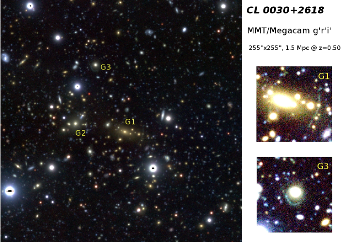
Figure 1: Three-colour composite of CL0030+2618, prepared from the Megacam $g^{\prime}r^{\prime}i^{\prime}$ coadded images. The main image shows a cut-out of the central region of CL0030+2618, with an edge length of $\approx\!255\arcsec$ ($1600\,\mbox{px}$), corresponding to the virial radius of $\approx\!1.5\,\mbox{Mpc}$ at the cluster redshift of $z\!=\!0.50$. North is up and East is to the left. The tentative luminous arcs near the galaxies G1 and G3 (Table LABEL:tab:gal and Sect. 5.4) are emphasized in the two smaller, zoomed ($40\arcsec\times 40\arcsec$) images.

In principle, the small distortions of background sources which we want to measure are achromatic. In practice, however, the optimal passband for weak lensing observations is determined by the signal-to-noise ratio which can be obtained in a given amount of time and depends on seeing and instrumental throughput. To maximise the number of high signal-to-noise, background galaxies whose shapes can be determined reliably for a given exposure time, we choose the $r^{\prime}$-band as the default lensing band. Aiming at a limiting magnitude of $r^{\prime}_{\mathrm{lim}}\!\approx\!26$ for $T_{\mathrm{exp}}\!\approx\!3\,\mbox{h}$, we obtain a sufficient number of high-quality shape sources ($n_{\mathrm{gal}}\!\gtrsim\!15\,\mbox{arcmin}^{-2}$) in the final catalogue.

Lensing effects depend on the relative distances between source and deflector (Bartelmann & Schneider 2001, Chap. 4.3). Ideally, we would like to determine a photometric redshift estimate for each galaxy in our lensing catalogue (e.g.: Benítez 2000; Bolzonella et al. 2000; Wolf et al. 2001; Ilbert et al. 2006; Hildebrandt et al. 2008). However, this is observationally expensive as deep imaging in $\gtrsim\!5$ passbands is necessary to obtain accurate photometric redshifts.

On the other hand, using only one filter (the lensing band) and a simple magnitude cut for a rough separation of background from foreground galaxies needs a minimum of observing time but neglects the galaxies’ intrinsic distribution in magnitude. We are following an intermediary approach here, using three filters from which we construct colour-colour-diagrammes of the detected galaxies and use this information to achieve a more accurate background selection than using the simplistic magnitude cut. This method has successfully been applied to weak-lensing galaxy cluster data by e.g. Clowe & Schneider (2002); Bradač et al. (2005); Kausch et al. (2007). Megacam’s $g^{\prime}$ and $i^{\prime}$ passbands straddle the Balmer break, the most distinctive feature in an elliptical galaxy’s optical spectrum in the redshift range $z\!\approx\!0.5$ in which we are interested. Therefore, we use the $g^{\prime}r^{\prime}i^{\prime}$ filters and resulting colours to identify foreground and cluster objects in our catalogues.

In order to obtain a high level of homogeneity in data quality over the field-of-view despite the gaps between Megacam’s chips, we stack dithered exposures. Our dither pattern consists of $5\!\times\!5$ positions in a square array with $40\arcsec$ distance between neighbouring points, inclined by $10\degr$ with respect to the right ascension axis on which the chips normally are aligned. We find this pattern to be robust against missing frames (exposures which couldn’t be used in the final stack for whatever reason).

2.4 The Data

The data presented in this paper have been collected in five nights distributed over two observing runs on October 6th and 7th, 2004 and October 30th, October 31st, and November 1st of 2005. In these two observing runs, a total of four 400d Cosmological Sample clusters have been observed. In the first phase of data reduction, the so-called run processing, these data have been processed in a consistent fashion. A weak lensing analysis of the three clusters besides CL0030+2618, namely CL0159+0030, CL0230+1836, and CL0809+2811, will be the topic of an upcoming paper in this series. In this work, we make use of part of these data for the photometric calibration of CL0030+2618 images (see Sect. 3.2.1).

In Table 1, we give the exposure times, seeings, and related information for the final image stacks on which we base all further analysis. Fig. 1 shows a three-colour composite image prepared from the stacked Megacam $g^{\prime}r^{\prime}i^{\prime}$ observations of CL0030+2618.

3 Outline of Data Reduction

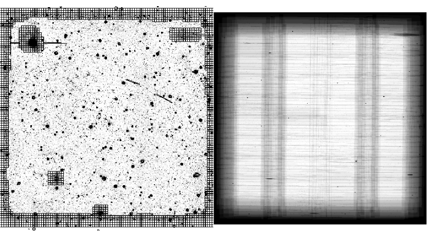
Figure 2: Left: The coadded $r^{\prime}$-band image of CL0030+2618, overlaid with its final masks. The target cluster is located in the frame centre. Small square masks cover regions masked because of their source counts strongly deviating from the average in the field (Sect. 3.1). The elongated masks enclose tracks of slowly moving objects (asteroids) which had to be identified on the image by visual inspection. The small octagonal masks are saturated stars found from the USNO B1 catalogue and manually. Right: The $r^{\prime}$-band weight image of CL0030+2618. Pixels lying in the interior of the chips get significantly higher weights than those which fall into an intra-chip gap in some of the dithered exposures.

Table 1: Specifications of the coadded images for CL0030+2618

Filter	Observation Dates	$T_{\mathrm{exp}}^{\mathrm{fin}}[s]$	Seeing	Calib. Method	$m_{\mathrm{lim}}$
r’	2004-10-06/7	6600	0.82	stellar colours	25.9
g’	2005-10-30/1, 2005-11-01	7950	0.87	SDSS standards	26.8
i’	2005-10-31	5700	1.03	SDSS standards	25.1

The reduction of the data presented in this paper relies on the THELI pipeline originally designed and tested on observations obtained using the Wide-Field Imager (WFI) on ESO’s La Silla 2.2 m telescope (Erben et al. 2005). While the reduction follows the procedure detailed in Erben et al. (2005), some important changes had to be made to adapt the THELI pipeline to work on MMT Megacam data. In the following discussion of the subsequent individual reduction routines, special emphasis has been given to those adaptations arising from the fact that MMT Megacam is a “new” camera with a small field-of-view per chip ($325\arcsec\!\times\!164\arcsec$ instead of $853\arcsec\!\times 379\!\arcsec$ for MegaPrime at CFHT, or a factor $1/6$ in field-of-view), using a larger telescope.

The THELI pipeline distinguishes two stages of data reduction: run processing and set processing. During run processing, the first phase, all frames taken during an observation run in a particular filter are treated in the same way. Run processing comprises the removal of instrumental signatures, e.g. de-biasing and flatfielding. In set processing the data are re-ordered according to their celestial coordinates rather than their date of observation. Astrometric and photometric calibration lead to a resulting “coadded” (stacked) image for each set. In Fig. 2, we present the coadded $r^{\prime}$-band image of CL0030+2618, overlaid with its final masks in the left and its weight image in the right part of the plot.

3.1 Coaddition “Post Production”

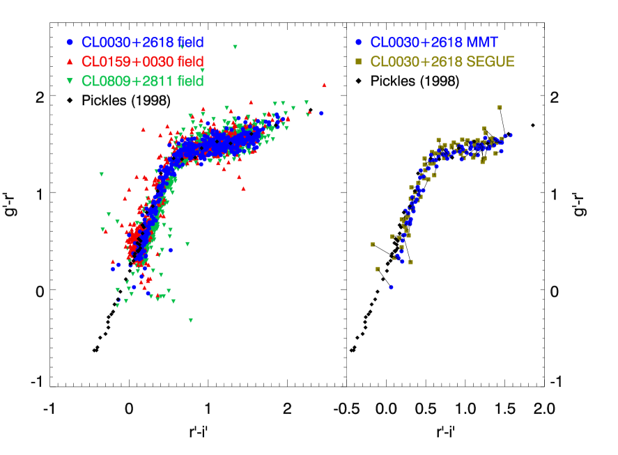
Figure 3: Photometric calibration by stellar colours: Left panel: plotted here are the $g^{\prime}\!-\!r^{\prime}$ vs. $r^{\prime}\!-\!i^{\prime}$ colours of sources identified as stars in three galaxy cluster fields observed with Megacam. For two of these fields, CL0159+0030 (upward triangles) and CL0809+2811 (downward triangles), absolute photometric calibration with SDSS standards could be performed. For CL0030+2618, results for recalibrated $r^{\prime}$-band zeropoints are shown (dots; details see main text) The colours in all three fields agree with the colours of main sequence stars from the Pickles (1998) spectral library (diamonds). Right panel: The $g^{\prime}\!-\!r^{\prime}$ vs. $r^{\prime}\!-\!i^{\prime}$ colours of stars in the Megacam images of CL0030+2618 (dots) which could also be identified in the partially overlapping SEGUE strip (Newberg & Sloan Digital Sky Survey Collaboration 2003) and shown here as squares are both consistent with each other as well as with the Pickles (1998) colours (diamonds). Each pair of measurements of one individual source is connected.

The final stage of the data reduction is to mask problematic regions in the coadded images, applying the methods presented in Dietrich et al. (2007). By subdividing the image into grid cells of a suitable size and counting SExtractor detections within those, we identify regions whose source density strongly deviate from the average as well as those with large gradients in source density. This method not only detects the image’s borders but also masks, effectively, zones of increased background close to bright stars, galaxies or defects.

In a similar fashion, we mask bright and possibly saturated stars which are likely to introduce spurious objects in catalogues created with SExtractor. We place a mask at each position of such sources as drawn from the USNO B1 catalogue. The method in which the size of the mask is scaled according to the star’s magnitude has been described in some detail in Erben et al. (2009). A small number of objects per field which are missing in the USNO B1 catalogue has to be masked manually while masks around catalogue positions where no source can be found have to be removed.

Conforming with Hildebrandt et al. (2005), we compute the limiting magnitudes in the coadded images for a $5\sigma$-detection in a $2\arcsec$ aperture as

$$m_{\mathrm{lim}}\!=\!Z_{f}-2.5\log{(5\sqrt{N_{\mathrm{pix}}}\sigma_{\mathrm{sky}})}$$ (2)

with $Z_{f}$ being the photometric zeropoint in the respective filter $f$, $N_{\mathrm{pix}}$ the number of pixels within the $2\arcsec$ aperture and $\sigma_{\mathrm{sky}}$ the RMS sky-background variation measured from the image.

Obtaining accurate colours for objects from CCD images is not as trivial as it might seem. Next to the photometric calibration (see Sect. 3.2), aperture effects have to be taken into account. Our approach is to measure SExtractor isophotal (ISO) magnitudes from seeing-equalised images in our three bands. We perform a simplistic PSF matching based on the assumption of Gaussian PSFs as it has been described in Hildebrandt et al. (2007): The width of the filter with which to convolve the $k$-th image is given as

$$\sigma_{\mathrm{filter,k}}=\sqrt{\sigma_{\mathrm{worst}}^{2}-\sigma_{\mathrm{k}}^{2}}$$ (3)

with $\sigma_{\mathrm{k}}$ and $\sigma_{\mathrm{worst}}$ being the widths of the best fitting Gaussians to the PSFs measured from the $k$-th and the worst seeing image.

3.2 Photometric Calibration

3.2.1 Calibration Pipeline

The photometric calibration of our data is largely based on the method developed by Hildebrandt et al. (2006) but using AB magnitudes and SDSS-like filters together with the SDSS Data Release Six (Adelman-McCarthy et al. 2008, DR6) as our calibration catalogue.

As mentioned in Sect. 2.4, the CL0030+2618 data we present here have been observed together with three other clusters from the 400d sample. Two of these, CL0159+0030 and CL0809+2811, are situated within the SDSS DR6 footprint. In addition to these, numerous Stetson (2000) standard fields were observed along with the science data of which some provide further SDSS photometry.

The MMT/Megacam filter system is based on the SDSS one but not identical to it (see Fig. 18); the comparison between the systems is detailed in Sect. A.5 in the Appendix. Therefore, relations between instrumental magnitudes and calibrated magnitudes in the SDSS system have to take into account colour terms.

In order to determine the photometric solution, we use SExtractor to draw catalogues from all science and standard frames having SDSS overlap. Using the Hildebrandt et al. (2006) pipeline, we then match these catalogues with a photometric catalogue assembled from the SDSS archives, serving as indirect photometric standards.

The relation between Megacam instrumental magnitudes $m_{\mathrm{inst}}$ and catalogue magnitudes $m_{\mathrm{SDSS}}$ for a filter $f$ can be fitted as a linear function of airmass $a$ and a first-order expansion with respect to the colour index, simultaneously:

$$m_{\mathrm{f,inst}}-m_{\mathrm{f,SDSS}}\!=\!\beta_{\mathrm{f}}(m_{\mathrm{f,SDSS}}-m_{\mathrm{f^{\prime},SDSS}})+\gamma_{\mathrm{f}}a+Z_{\mathrm{f}}$$ (4)

where $m_{\mathrm{f,SDSS}}-m_{\mathrm{f^{\prime},SDSS}}$ is a general colour index w.r.t. another filter $f^{\prime}$, $\beta_{\mathrm{f}}$ the corresponding colour term, and $Z_{\mathrm{f}}$ the photometric zeropoint in which we are mainly interested. For the fit, we select objects of intermediate magnitude which are neither saturated nor show a too large scatter in $m_{\mathrm{inst}}$ given a certain $m_{\mathrm{SDSS}}$. Following the model of Hildebrandt et al. (2006), we account for the variable photometric quality of our data by fitting $\beta_{\mathrm{f}}$, $\gamma_{\mathrm{f}}$, and $Z_{\mathrm{f}}$ simultaneously under the best conditions, fixing $\gamma_{\mathrm{f}}$ in intermediate, and fixing $\gamma_{\mathrm{f}}$ and $\beta_{\mathrm{f}}$ in even poorer conditions. The fixed extinctions and colour terms are set to default values which are discussed in Sect. A.5 in the Appendix.

3.2.2 Colour-Colour-Diagrammes

Comparing the zeropoints for different nights and fields, we conclude that the nights on which the $r^{\prime}$-band observations of CL0030+2618 were performed, were not entirely photometric but show a thin, uniform cirrus. Therefore, an indirect re-calibration method is needed here. To this end, we fitted the position in the $r^{\prime}\!-\!i^{\prime}$ vs. $g^{\prime}\!-\!r^{\prime}$ colour-colour-diagramme of the stars identified in the CL0030+2618 field to those found in two other, fully calibrated, galaxy cluster fields, CL0159+0030 and CL0809+2811.

In the left panel of Fig. 3, we plot the $g^{\prime}\!-\!r^{\prime}$ versus $r^{\prime}\!-\!i^{\prime}$ colours of stars identified in these two fields and compare them to theoretical spectra of main-sequence stars from the Pickles (1998) spectral library to find good agreement between both the two observed sequences and the predicted stellar colours.

As we find reliable absolute photometric calibrations for the $g^{\prime}$- and $i^{\prime}$-bands of CL0030+2618, the location of the stellar main sequence for this field is determined up to a shift along the main diagonal of the $g^{\prime}\!-\!r^{\prime}$ versus $r^{\prime}\!-\!i^{\prime}$ diagramme, corresponding to the $r^{\prime}$ zeropoint. We fix this parameter by shifting the main sequence of CL0030+2618 on top of the other observed main sequences as well as the Pickles (1998) sequence. We go in steps of 0.05 magnitudes, assuming this to be the best accuracy we can reach adopting this rather qualitative method and settle for the best-fitting test value (see Table 1). The dots in Fig. 3 show the best match with the CL0159+0030 and CL0809+2811 stellar colours obtained by the re-calibration of the CL0030+2618 $r^{\prime}$-band.

After the photometric calibration, we became aware of a field observed in the SEGUE project (Newberg & Sloan Digital Sky Survey Collaboration 2003) using the SDSS telescope and filter system which became publicly available along with the Sixth Data Release of SDSS (Adelman-McCarthy et al. 2008) and partially overlaps with the CL0030+2618 Megacam observations. Thus, we are able to directly validate the indirect calibration by comparing the colours of stars in the overlapping region. The right panel of Fig. 3 shows the good agreement between the two independent photometric measurements and the Pickles (1998) templates from which we conclude that our calibration holds to a good quality.

For comparison we also calibrated the CL0030+2618 $r^{\prime}$-band by comparing its source counts to the ones in the CL0159+0030 and CL0809+2811 fields for the same filter, but discard this calibration as we find a discrepancy of the resulting main sequence in $g^{\prime}\!-\!r^{\prime}$ versus $r^{\prime}\!-\!i^{\prime}$ with the theoretical Pickles (1998) models mentioned earlier.

4 The Shear Signal

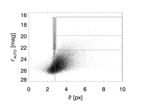
Figure 4: The distribution of sources in the apparent size – magnitude – space. Plotted are the SExtractor magnitudes $r^{\prime}_{\mathrm{AUTO}}$ against the half-light radii $\vartheta$ of all sources in the “reliable” catalogue. The stellar locus is visible prominently and is defined for further analysis by $2.55\leavevmode\nobreak\ \mbox{px}\!<\vartheta\!<\!2.95\leavevmode\nobreak\ \mbox{px}$ and $16.75\leavevmode\nobreak\ \mbox{mag}\!<\!r^{\prime}_{\mathrm{AUTO}}\!<\!22.5\leavevmode\nobreak\ \mbox{mag}$ (the grey shaded area). The sources to the right and lower sides of the thick lines $r^{\prime}_{\mathrm{AUTO}}\!<\!16.75\leavevmode\nobreak\ \mbox{mag}$ and $\vartheta\!>\!2.8\leavevmode\nobreak\ \mbox{px}$ for sources fainter than $22.5\leavevmode\nobreak\ \mbox{mag}$ we treat as unsaturated galaxies. In addition, the magnitude limits $m_{\mathrm{bright}}$ and $m_{\mathrm{faint}}$ defined in Sect. B.2 are given as thin lines for illustrative purposes.

Gravitational lensing leads to a distortion of images of distant sources by tidal gravitational fields of intervening masses. Here, we describe the method to measure this shear while referring to Schneider (2006) for the basic concepts and notation.

4.1 KSB analysis

The analysis of the weak lensing data is based on the Kaiser et al. (1995, KSB) algorithm. The reduction pipeline we use was adapted from the “TS” implementation presented in Heymans et al. (2006) and explored further in Schrabback et al. (2007); Hartlap et al. (2009). Its basic concepts are already outlined in Erben et al. (2001). Thus, in this section, we will focus more on the properties of our data than on the methods themselves since they are well documented in the above references.

The KSB algorithm confronts the problem of reconstructing the shear signal from measured galactic ellipticities; therefore, it has to disentangle the shear $\gamma$ from the intrinsic ellipticities of the galaxies and from PSF effects. The simultaneous effects of shear dilution by the PSF and the superposition of the incoming ellipticity with the anisotropic PSF component can be isolated by tracing the shapes of sources we can identify as stars, bearing neither intrinsic ellipticity nor lensing shear.

The complete correction yielding a direct, and ideally unbiased, estimator $\varepsilon$ of the (reduced) shear $g$ exerted on a galaxy in our catalogue reads:

$$\varepsilon_{\alpha}=\left(\@tens{P}^{\mathrm{g}}\right)^{-1}_{\alpha\beta}\left[e_{\beta}-\@tens{P}^{\mathrm{sm}}_{\beta\gamma}\left(\left(\@tens{P}^{\mathrm{sm*}}\right)^{-1}_{\gamma\delta}e^{*}_{\delta}\right)\right]$$ (5)

Here, small Greek indices denote either of the two components of the complex ellipticity. Quantities with asterisks are measured from stellar sources. The $e_{\beta}$ are the ellipticities of galaxies as measured from the input “shape” image while the $e^{*}_{\delta}$ are the ellipticities of stars tracing the PSF (plotted in the left two panels of Fig. 5). The $2\times 2$ matrices $\@tens{P}^{\mathrm{g}}$ and $\@tens{P}^{\mathrm{sm}}$ give the transformation of ellipticities under the influences of gravitational shear fields and the presence of an (anisotropic) PSF, respectively. See, e.g., Schneider (2006) on how these quantities are determined from higher-order moments of the measured brightness distributions.

4.2 The KSB and Galaxy Shape Catalogues

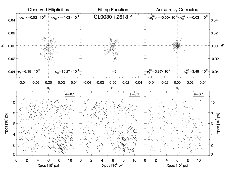
Figure 5: Correction of PSF anisotropy of the CL0030+2618 $r^{\prime}$ band as used in the analysis. The upper panel shows the distribution of the ellipticity components $e_{1,2}$ of the stars identified in the field, together with the numeric values of their dispersions $\sigma_{1,2}\!:=\!\sigma(e_{1,2})$. The “whisker plots” in the lower panel show the size and orientation of PSF anisotropy as they vary as a function of the spatial coordinates $x$ and $y$. On the left, the situation before correction, i.e. the ellipticities as measured in the stars are depicted. The middle two plots give the fit by a global fifth order polynomial in $x$ and $y$. Residuals of this correction are presented in the plots on the right.

Catalogues are created from the images using the SExtractor double detection mode: Sources are identified on the lensing band image in its original seeing. Photometric quantities (fluxes, magnitudes) are determined at these coordinates from the measurement images in the three bands $g^{\prime}r^{\prime}i^{\prime}$ convolved to the worst seeing (found in the $i^{\prime}$-band).

The photometric properties determined from the three bands are merged into one catalogue based on the detection image. From those catalogues problematic sources are removed. Those are sources near the boundaries of the field-of-view or blended with other sources, as well as objects whose flux radii do not fall in the range $\vartheta^{*}\!<\!\vartheta_{\mathrm{g}}\!<\!10\leavevmode\nobreak\ \mbox{px}$, for which KSB works safely, with $\vartheta^{*}$ the angular size of unsaturated stars. For the remaining objects, the shapes can now be determined.

Note that the KSB catalogue presented in Fig. 4 and all catalogues discussed hereafter only contain those objects for which a half-light radius $\vartheta$ could be determined by our implementation of the Erben et al. (2001) method. Objects for which the measurements on the (noisy) data yield negative fluxes, semi major axes, or second-order brightness moments or which lie to close to the image border are removed from the catalogue, reducing its size by $\sim\!3$ %.

Figure 4 shows the distribution of the sources in the “reliable” catalogue in apparent size – magnitude space. The prominent stellar locus enables us to define a sample of stars by $\vartheta^{*}_{\mathrm{min}}\!\!<\!\vartheta\!\!<\!\vartheta^{*}_{\mathrm{max}}$ and $r^{\prime*}_{\mathrm{min}}\!<\!r^{\prime}_{\mathrm{AUTO}}\!<\!r^{\prime*}_{\mathrm{max}}$ with $\vartheta^{*}_{\mathrm{min}}\!\!=\!2.55\leavevmode\nobreak\ \mbox{px}$, $\vartheta^{*}_{\mathrm{max}}\!\!=\!2.95\leavevmode\nobreak\ \mbox{px}$, $r^{\prime*}_{\mathrm{min}}\!\!=\!16.75\leavevmode\nobreak\ \mbox{mag}$, and $r^{\prime*}_{\mathrm{max}}\!\!=\!22.5\leavevmode\nobreak\ \mbox{mag}$ (the shaded area in Fig. 4) from which the PSF anisotropy $e^{*}_{\delta}$ in Eq. (5) is determined.

In the transition to the galaxy shape catalogue, we regard as unsaturated galaxies all objects $r^{\prime}_{\mathrm{AUTO}}\!>\!r^{\prime*}_{\mathrm{min}}$ (i.e. fainter than the brightest unsaturated point sources) and more extended than $\vartheta\!\!>\!\vartheta^{*}_{\mathrm{max}}$ for $r^{\prime}_{\mathrm{AUTO}}\!\!<\!r^{\prime*}_{\mathrm{max}}$ or $\vartheta\!\!>\!2.8\leavevmode\nobreak\ \mbox{px}$ for $r^{\prime}_{\mathrm{AUTO}}\!\!>\!r^{\prime*}_{\mathrm{max}}$, respectively. The latter is justified by the fact that while for bright sources it is easy to distinguish galaxies from point sources, there is a significant population of faint galaxies for which a very small radius is measured by the SExtractor algorithm. Thus, we relax the radius criterion by $5$ % for sources fainter than $r^{\prime*}_{\mathrm{max}}$.

However, we notice that among those small objects there is a population of faint stars, not distinguishable from poorly resolved galaxies using an apparent size – magnitude diagramme alone and resulting in a dilution of the lensing signal compared to a perfect star – galaxy distinction. Our decision to nevertheless include these small sources into our catalogue is based on the resulting higher cluster signal as compared to a more conservative criterion (e.g. $\vartheta/\vartheta^{*}_{\mathrm{max}}\!\leq\!1.10$ for the galaxies fainter than $r^{\prime*}_{\mathrm{max}}$). We call “galaxy shape catalogue” the list of objects that both pass this galaxy selection and the cuts for signal quality discussed in Sect. 4.6. This important catalogue yields the final “lensing catalogue” by means of the background selection discussed in Sect. 4.4.

4.3 PSF Anisotropy of Megacam

Figure 6: The effect of the polynomial correction for the PSF anisotropy on the ellipticities of galaxies averaged in equally populated bins. As a function of the amount of correction $e^{\mathrm{cor}}$ applied to the components $\delta\!=\!1$ (left panels) and $\delta\!=\!2$ (right panels), we show the raw ellipticities before correction in the upper panels and the PSF-corrected ellipticities $\varepsilon$ in the lower panels. The bars in the abscissa and ordinate denote the range of the bin and the standard deviation of the ellipticity in this bin, respectively.

In the KSB pipeline, we fit a model $e^{\mathrm{cor},*}(x,y)$ in the pixel coordinates $x$ and $y$ to the measured ellipticities $e^{*}$ of stars such that the residual anisotropies $e^{\mathrm{ani},*}\!=e^{*}\!-\!e^{\mathrm{cor},*}$ of stellar images should effectively be zero. Figure 5 shows the effect of PSF anisotropy correction: The raw ellipticities of the tracing stars as presented in the left two panels are modelled by a polynomial $e^{\mathrm{cor}}\!=\!\sum_{k=0}^{n}{\sum_{\ell=0}^{n-k}{p_{k\ell}x^{k}y^{\ell}}}$ defined globally over the whole field-of-view. The best-fitting solution for the case $n\!=\!5$ we adopt here is shown in the middle panels of Fig. 5 while the residual ellipticities of the stars $e^{\mathrm{ani}}$ are displayed in the panels to the right.

Simultaneously aiming at reducing both the mean $\langle e^{\mathrm{ani,*}}_{\delta}\rangle$ of the residual ellipticities and their dispersion $\sigma(e^{\mathrm{ani,*}}_{\delta})$ we find that a polynomial order as high as $n\!=\!5$ is necessary to effectively correct for the distinctive quadrupolar pattern in the spatial distribution of the “raw” stellar ellipticities (see lower left and middle panels of Fig. 5). There is no obvious relation between the zones of preferred orientation of the PSF ellipticity in Fig. 5 and the $4\times 9$ chip detector layout of Megacam. See Sect. 4.6 for further details.

For stacking in the lensing band, we select only those frames which show moderate PSF ellipticity in the first place (see Sect. A.4 in the Appendix for details). Thus, we ensure the images used for lensing analysis to be isotropic to a high degree even before any corrections are applied. By stacking images in which the PSF anisotropy is different in magnitude and orientation (cf. Figs. 16 and 17), we further reduce the ellipticity owing to the imaging system. The total amount of PSF anisotropy present in our Megacam data is small: Before correction, we measure $\langle e_{1}\rangle\!=\!1.77\times 10^{-5}$, $\langle e_{2}\rangle\!=\!-4.03\times 10^{-3}$, $\langle|e|\rangle=\!1.10\times 10^{-2}$, and $\sigma(|e|)\!=\!6.19\times 10^{-3}$, reducing after the correction to $\langle e^{\mathrm{ani}}_{1}\rangle\!=\!-5.60\times 10^{-7}$, $\langle e^{\mathrm{ani}}_{2}\rangle\!=\!-2.60\times 10^{-5}$, $\langle|e^{\mathrm{ani}}|\rangle=\!4.34\times 10^{-3}$, and $\sigma(|e^{\mathrm{ani}}|)\!=\!2.90\times 10^{-3}$. Note that the very small averages for the individual components result from partial cancellation of anisotropies from different parts of the field-of-view. Thus, MMT/Megacam shows a similar degree of PSF anisotropy as other instruments from which lensing signals have been measured successfully, e.g. MegaPrime/Megacam on CFHT (Semboloni et al. 2006) or Subaru’s SuprimeCam (Okabe & Umetsu 2008). The latter authors measured, as an RMS average of seven galaxy cluster fields, $\langle e_{1}\rangle\!=\!1.41\times 10^{-2}$, $\langle e_{2}\rangle\!=\!1.63\times 10^{-2}$, and $\sigma(|e|)\!=\!2.32\times 10^{-2}$ before correction with larger values for the anisotropy components but a simpler spatial pattern.

Although we find small-scale changes in the PSF ellipticity which have to be modelled by a polynomial of relatively high order, the more important point is that the PSF anisotropy varies smoothly as a function of the position on the detector surface in every individual exposure, showing a simpler pattern than Fig. 5. (See Fig. 17 for example exposures at both small and large values of overall PSF anisotropy induced by the tracking behaviour of MMT.) Consequently, it can be modelled by a smooth function which is a necessary prerequisite for using the instrument with the current weak lensing analysis pipelines. Thus, we have shown that weak lensing work is feasible using MMT Megacam.

4.4 Selection of lensed background galaxies

Before we proceed with the details of our lensing analysis, we explain how we arrive from the galaxy shape catalogue at the “lensing catalogue” of objects we classify as background galaxies w.r.t. to CL0030+2618. This background selection, as we will call it from now on= is based on their $g^{\prime}r^{\prime}i^{\prime}$ photometry. While unlensed objects remaining in the catalogue dilute the shear signal, rejection of actual background galaxies reduce it as well. Note that a sensible foreground removal is especially important for relatively distant objects like the 400d Cosmology Sample clusters.

We introduce two free parameters in our analysis: the magnitude limit $m_{\mathrm{faint}}$ below which all fainter galaxies are included in the shear catalogue, regardless of their $g^{\prime}\!-\!r^{\prime}$ and $r^{\prime}\!-\!i^{\prime}$ colour indices, and the magnitude $m_{\mathrm{bright}}$ above which all brighter galaxies will be considered foreground objects and discarded. Only in the intermediary interval $m_{\mathrm{bright}}\!<\!r^{\prime}\!<\!m_{\mathrm{faint}}$ the selection of galaxies based on their position in the colour-colour-diagramme will take place. In these terms, a simple magnitude cut would correspond to $m_{\mathrm{bright}}\!=\!m_{\mathrm{faint}}$. We vary these parameters in order to optimise the detection of CL0030+2618 and find $m_{\mathrm{bright}}\!=\!20.0$ and $m_{\mathrm{faint}}\!=\!22.5$. For details of the colour-colour-diagramme method, see Sect. B.2. The photometric cuts reduce the catalogue size by $6.0$ %, leaving us with a lensing catalogue of $N_{\mathrm{cat}}\!=\!14813$ objects, corresponding to a galaxy surface density of $n_{\mathrm{cat}}\!=\!21.2\,\mbox{arcmin}^{-2}$.

4.5 Aperture mass and lensing detection

The weak lensing analysis we conduct is a two-step process. First, we confirm the presence of a cluster signal by constructing aperture mass maps of the field which will provide us with a position for the cluster centre and the corresponding significance. In the second step, building on this position for CL0030+2618, the tangential shear profile can be determined and fitted, leading to the determination of the cluster mass.

More precisely, we use the so-called $S$-statistics, corresponding to the signal-to-noise ratio of the aperture mass estimator which for any given centre $\boldsymbol{\theta}_{\mathrm{c}}$ is a weighted sum over the tangential ellipticities of all lensing catalogue galaxies within a circular aperture of radius $\theta_{\mathrm{out}}$. The estimator can be written analytically as (Schneider 1996):

$$S_{\theta_{\mathrm{out}}}(\boldsymbol{\theta}_{\mathrm{c}})\!=\!\frac{\sqrt{2}}{\sigma_{\varepsilon}}\frac{\sum_{i}{\varepsilon_{\mathrm{t},i}Q_{i}(|\boldsymbol{\theta}_{\mathrm{i}}\!-\!\boldsymbol{\theta}_{\mathrm{c}}|)}}{\sqrt{\sum_{i}{Q_{i}^{2}(|\boldsymbol{\theta}_{\mathrm{i}}\!-\!\boldsymbol{\theta}_{\mathrm{c}}|)}}}$$ (6)

where $\varepsilon_{\mathrm{t},i}$ denotes the measured shear component tangential with respect to the centre for the galaxy at position $\boldsymbol{\theta}_{\mathrm{i}}$. As filter function $Q(x\!:=\!|\boldsymbol{\theta}_{\mathrm{i}}\!-\!\boldsymbol{\theta}_{\mathrm{c}}|/\theta_{\mathrm{out}})$, we apply the hyperbolic tangent filter introduced by Schirmer et al. (2007):

$$Q_{\mathrm{TANH}}(x)\!=\!\frac{1}{1+\mathrm{e}^{a-bx}+\mathrm{e}^{c+dx}}\frac{\tanh{(x/x_{\mathrm{c}})}}{x/x_{\mathrm{c}}}$$ (7)

with the width of the filter determined by $x_{\mathrm{c}}\!=\!0.15$ and the shape of its exponential cut-offs for small and large $x$ given by the default values $\{a,b,c,d\}\!=\!\{6,150,47,50\}$. The $S$-statistics includes as a noise term the intrinsic source ellipticity, calculated from the data galaxies as $\sigma_{\varepsilon}\!=\!\langle\varepsilon_{1}^{2}\!+\!\varepsilon_{2}^{2}\rangle^{1/2}$ with typical values $\sigma_{\varepsilon}\!\approx\!0.38$.

The value of $\theta_{\mathrm{out}}$ in Eq. (6) is also fixed such that it maximises $S_{\theta_{\mathrm{out}}}(\boldsymbol{\theta}_{\mathrm{c}})$ which strongly depends on the filtering size used. Exploring the parameter space spanned by $\theta_{\mathrm{out}}$ and the photometric parameters $m_{\mathrm{bright}}$ and $m_{\mathrm{faint}}$, we find, independent of the latter two, the highest $S$-values with $14\arcmin\!<\!\theta_{\mathrm{out}}\!<\!15\arcmin$. The behaviour of $S$ as a function of $\theta_{\mathrm{out}}$ (at a fixed $\boldsymbol{\theta}_{\mathrm{c}}$) is in good general agreement with the results of Schirmer et al. (2007) for the same filter function $Q_{\mathrm{TANH}}(x)$. Thus, we fix $\theta_{\mathrm{out}}\!=\!14\aas@@fstack{\prime}5$ for the further analysis, noting this number’s agreement with the size of our Megacam images (cf. Fig. 8). We also tested the influence of the parameter $x_{\mathrm{c}}$ in the $Q_{\mathrm{TANH}}$ filter and find that, with all other parameters kept fixed, in the $0.15\!\leq\!x_{\mathrm{c}}\!\leq 0.6$ interval the maximum $S$-value changes by less than 0.5 % but decreases more steeply for smaller values of $x_{\mathrm{c}}$.

Applying these parameters and measuring $S$ on a reference grid of $60\arcsec$ mesh size, we detect CL0030+2618 at the level of $5.8\sigma$ in a grid cell centred at a distance of $34\arcsec$ from the ROSAT position at $\alpha_{\mathrm{J2000}}\!=\!00^{\mathrm{h}}30^{\mathrm{m}}33\aas@@fstack{s}6,\delta_{\mathrm{J2000}}\!=\!26\degr 18\arcmin 16\arcsec$, i.e. smaller than the grid resolution. We will investigate further into the cluster position in Sect. 5.2.

4.6 Verification of the shear signal

Figure 7: The $S$-statistics (solid line) as a function of the maximum value of the ellipticity estimator $\varepsilon$ resulting we include in the galaxy shape catalogue. The dashed and dash-dotted lines show the sizes of the resulting catalogue before and after background selection (see Sect. B.2), respectively.

Table 2: Notable galaxies in the field of CL0030+2618.

Galaxy	$\alpha_{\mathrm{J2000}}$	$\delta_{\mathrm{J2000}}$	$r^{\prime\mathrm{MMT}}_{\mathrm{AUTO}}$	$g^{\prime\mathrm{MMT}}_{\mathrm{AUTO}}$	$i^{\prime\mathrm{MMT}}_{\mathrm{AUTO}}$	$z$	Note	See Figure
G1	$00^{\mathrm{h}}30^{\mathrm{m}}34\aas@@fstack{s}0$	$26\degr 18\arcmin 09\arcsec$	$19.20$	$21.14$	$18.31$	$0.516^{\dagger}$	dominant in CL0030+2618	Fig. 1
G2	$00^{\mathrm{h}}30^{\mathrm{m}}37\aas@@fstack{s}9$	$26\degr 18\arcmin 18\arcsec$	$18.82$	$20.23$	$18.27$	n.a.	dominant in foreground group	Fig. 1
G3	$00^{\mathrm{h}}30^{\mathrm{m}}36\aas@@fstack{s}3$	$26\degr 19\arcmin 20\arcsec$	$19.46$	$20.76$	$18.95$	n.a.	strong lensing feature	Fig. 1
G4	$00^{\mathrm{h}}30^{\mathrm{m}}39\aas@@fstack{s}5$	$26\degr 20\arcmin 56\arcsec$	$17.23$	$17.98$	$16.94$	$0.493^{\dagger}$	QSO	Fig. 9

^† Redshift taken from Boyle et al. (1997).

In this subsection, we summarise the consistency tests performed on the data to validate the galaxy shape measurements giving rise to the shear signal discussed below.

• Correction of PSF anisotropy: We assess the performance of the correction polynomial by analysing the PSF-corrected ellipticities $e^{\mathrm{ani}}_{\mathrm{gal},\delta}$ of galaxies as a function of the amount of correction $e^{\mathrm{cor}}_{\delta}$ that has been applied to them by fitting a polynomial to the anisotropy distribution of star images (see Sect. 4.3). Theoretically, the expected positive correlation between the uncorrected ellipticities and the correcting polynomial should be removed and $e^{\mathrm{ani}}_{\mathrm{gal}}(e^{\mathrm{cor}})$ thus scatter around zero. We note that most anisotropy is found in the $\delta\!=\!2$ component from the beginning (Fig. 6). This is removed in the corrected ellipticities, with $\langle e^{\mathrm{ani}}_{\mathrm{gal,2}}\rangle\!=\!-0.0010\!\pm\!0.0010$ marginally consistent with zero in the standard deviation. In the $\delta\!=\!1$ component, we measure a residual anisotropy of $\langle e^{\mathrm{ani}}_{\mathrm{gal,1}}\rangle\!=\!-0.0026\!\pm\!0.0010$ which is one order of magnitude smaller than the lensing signal we are about to measure.

  Alternatively to the $n\!=\!5$ polynomial correction to the entire image, we consider a piecewise solution based on the pattern of preferred orientation in Fig. 5. Dividing the field into four regions at $y\!=\!6100\,\mbox{px}$ and at $x\!=\!4300\,\mbox{px}$ for $y\!<\!6100\,\mbox{px}$ and $x\!=\!5800\,\mbox{px}$ for $y\!>\!6100\,\mbox{px}$ with a polynomial degree up to $n\!=\!5$ we do not find a significant improvement in terms of $\langle e^{\mathrm{ani,*}}\rangle$, $\sigma(e^{\mathrm{ani,*}})$, or $e^{\mathrm{ani}}_{\mathrm{gal}}(e^{\mathrm{cor}})$ over the simpler model defined over the whole field.

• Maximum shear: Due to the inversion of the noisy matrix $\@tens{P}^{\mathrm{g}}$ in Eq. (5), resulting values for the estimator $|\varepsilon|$ are not bound from above while ellipticities are confined to $0\!\leq\!e\!\leq\!1$. Thus, attempting to measure weak lensing using the KSB method, we need to define an upper limit $\max{(|\varepsilon|)}$ of the shear estimates we consider reliable. We evaluate the influence of the choice for $\max{(|\varepsilon|)}$ on the $S$-statistics (Eq. 6) by varying it while keeping the other parameters, like $\min{(\operatorname{tr}{\@tens{P}^{\mathrm{g}}})}$, the minimum $\min{(\nu)}$ of the signal-to-noise ratio $\nu$ of the individual galaxy detection determined by the KSB code, and the photometric parameters $m_{\mathrm{bright}}$ and $m_{\mathrm{faint}}$ defined in Sect. B.2 fixed. In the range $0.6\!\lesssim\!\max{(|\varepsilon|)}\!\lesssim\!0.8$, we find an increasing shear signal due to the higher number of galaxies in the catalogues using less restrictive cuts (Fig. 7). For $\max{(|\varepsilon|)}\!\gtrsim\!0.8$, we see a sharp decline of the lensing signal which we explain as an effect of galaxies entering the catalogue whose ellipticity estimate is dominated by noise. We fix $\max{(|\varepsilon|)}\!=\!0.8$, $\min{(\operatorname{tr}{\@tens{P}^{\mathrm{g}}})}\!=\!0.1$, and $\min{(\nu)}\!=\!4.5$ simultaneously to their given values. We note that, while optimising the $S$-statistics, this might introduce a bias in the mass estimate as a cut in $\max{(|\varepsilon|)}\!=\!0.8$ directly affects the averaging process yielding the shear.

• Shear calibration: We can account for this bias by scaling the shear estimates with a shear calibration factor $f$ such that $\varepsilon\!\rightarrow\!f_{0}\varepsilon$ to balance biases like the effect of $\max{(|\varepsilon|)}$. The question how gravitational shear can be measured unbiased and precisely has been identified as the crucial challenge to future weak lensing experiments (see e.g., Heymans et al. 2006; Massey et al. 2007; Bridle et al. 2009). The “TS” KSB method employed here has been studied extensively and is well understood in many aspects. In order to correct for the biased shear measurements, found by testing the KSB pipeline with the simulated data in Heymans et al. (2006), the shear calibration factor has been introduced and studied subsequently (Schrabback et al. 2007; Hartlap et al. 2009). As pointed out by these authors, the calibration bias depends on both the strength of the shear signal under inspection, as well as on the details of the implementation and galaxy selection for the shear catalogue. In the absence of detailed shape measurement simulations under cluster lensing conditions, we chose a fiducial $f_{0}\!=\!1.08$ from Hartlap et al. (2009) and assign an error of $\sigma_{\mathrm{f_{0}}}\!=\!0.05$ to it, covering a significant part of the discussed interval.

• Complementary catalogue: We check the efficacy of the set of parameters we adopted by reversing the selection of galaxies and calculating the $S$-statistics from those galaxies excluded in our normal procedure. Reversing the background selection, i.e. only keeping those galaxies regarded as cluster or foreground sources, we find from $10^{5}$ bootstrap realisations of the complentary catalogue an aperture mass significance of $S\!=\!-0.83\pm 1.06$. From the consistency with zero, we conclude these cuts to effectively select the signal-carrying galaxies. As the background selection removes $f_{\mathrm{ph}}\!=\!N_{\mathrm{complem}}/N_{\mathrm{cat}}\!=\!6.0$ % of the sources in the catalogue, we only expect a small bias $\approx\!f_{\mathrm{ph}}S_{\mathrm{complem}}/S_{\mathrm{cat}}\!\approx\!-0.8$ % resulting from the background selection.

Table 3: Colours of prominent galaxies observed in the CL0030+2618 field compared to colours computed from CWW80 elliptical templates at $z\!=\!0.50$ and $z\!=\!0.25$.

Galaxy	$z$	$g^{\prime}\!-\!i^{\prime}$	$g^{\prime}\!-\!r^{\prime}$	$r^{\prime}\!-\!i^{\prime}$
G1	$0.516$	$2.83$	$1.94$	$0.89$
G2	n.a.	$1.96$	$1.41$	$0.55$
CWW80 Ell $z\!=\!0.50$	$0.50$	$2.782$	$1.876$	$0.906$
CWW80 Ell $z\!=\!0.25$	$0.25$	$2.098$	$1.554$	$0.544$

5 The Multi-Wavelength View of CL0030+2618

5.1 Identifying the BCG of CL0030+2618

Figure 1 shows two candidates for the brightest cluster galaxy of CL0030+2618, galaxies with extended cD-like haloes and similar $i^{\prime}$-magnitudes (Table LABEL:tab:gal). The galaxy G1, closer to the Rosat and Chandra centres of CL0030+2618, was attributed to a cluster by Boyle et al. (1997), measuring a spectroscopic redshift of $z_{\mathrm{G1}}\!=\!0.516$, while three of their six spectro-$z$s are $z\!\approx\!0.25$.

We note that G1 and G2 show different colours in Fig. 1, each being similar to their fainter immediate neighbours. As very extended sources, G1 and G2 are flagged early-on in the pipeline but are included in the raw SExtractor catalogues. Aware of their larger uncertainties, we use these magnitudes for G1, G2, and two other interesting extended galaxies (Table LABEL:tab:gal).

The observed $g^{\prime}\!-\!r^{\prime}$, $r^{\prime}\!-\!i^{\prime}$, and $g^{\prime}\!-\!i^{\prime}$colours are compared to the ones predicted for a typical BCG at $z\!=\!0.50$ and $z\!=\!0.25$, using the Coleman et al. (1980, CWW80) elliptical galaxy template (Table LABEL:tab:galcww). Nicely consistent with its spectroscopic redshift, we find the colours of G1 to be similar to the $z\!=\!0.50$ template, while G2’s bluer colours resemble the CWW template at $z\!=\!0.25$. We conclude that G1, located close to the X-ray centres, is a member of CL0030+2618, and indeed its BCG. On the other hand, G2 can be considered the brightest member of a foreground group at $z\!\approx\!0.25$. The existence of such foreground structure is corroborated by the broad $g^{\prime}\!-\!i^{\prime}$ distribution (Fig. 19). Its implications are discussed in Sect. 5.2 and 6.3.1.

5.2 Comparing Centres of CL0030+2618

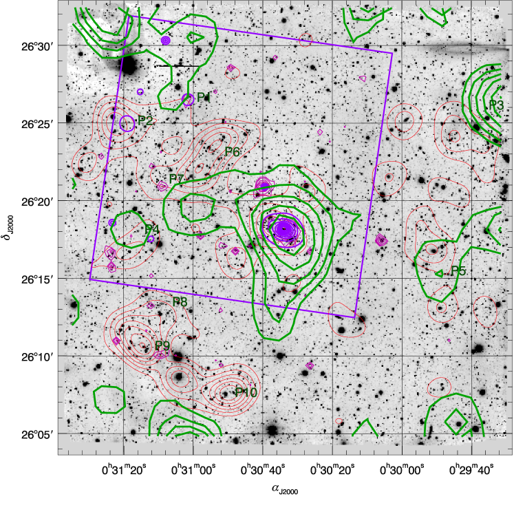
Figure 8: The $r^{\prime}$-band image of CL0030+2618, overlaid with $r^{\prime}$-band galaxy light (thin, red), Chandra (medium-thick, blue; within the smaller square footprint), and XMM-Newton (medium-thin, magenta), and lensing surface mass density contours (thick, green). We show X-ray surface brightness levels in multiples of $5\times 10^{-9}\mbox{cts}\,\mbox{cm}^{-2}\mbox{s}^{-1}\mbox{arcmin}^{-2}$ in the $0.5\ldots 2.\,\mbox{keV}$ band. The $r^{\prime}$-band flux density contours (thin red lines) start from $0.015$ flux units per pixel, in intervals of $0.005$ flux units. Lensing convergence contour levels were obtained smoothing the shear field $\gamma(\@vec{\theta})$ with a Gaussian filter of $2\arcmin$ width and are linearly spaced in intervals of $\Delta\kappa\!=\!0.01$, starting at $\kappa\!=\!0.01$. XMM-Newton contours show MOS2 counts smoothed by an adaptive Gaussian kernel in logarithmic spacing. The labels “P1” to “P10” designate the peaks discussed in Sect. 5.3.

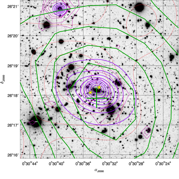
Figure 9: Zoomed version of Fig. 8, showing only the central region of CL0030+2618.The cross gives the position and $1\sigma$ uncertainty of the centre position of the $S$-peak obtained by bootstrapping (cf. Sect. 5.2) while the star symbols with five and six points denote the X-ray centres found with ROSAT and Chandra, respectively. The source on the northern edge on which strong X-ray emission is centred is named G4 in Table LABEL:tab:gal.

The $S$-statistics lensing centre

We determine the centre of the CL0030+2618 lensing signal and its accuracy by bootstrap resampling of the galaxy catalogue of $N_{\mathrm{cat}}$ galaxies used in the measurements of the $S$-statistics. From the basic catalogue we draw $10^{5}$ realisations each containing $N_{\mathrm{cat}}$ sources. For each realisation, we determine the $S$-statistics in the central region of $3\arcmin\!\times\!3\arcmin$ side length ($\sim\!\!1\mbox{Mpc}$ or roughly the virial radius of CL0030+2618) using a gridsize of $15\arcsec$ and record the highest $S$-value found on the grid and the grid cell in which it occurs.

Re-running $10^{5}$ bootstrap realisations of the lensing catalogue with the centre fixed to the lensing centre, we calculate a detection significance of $S(\boldsymbol{\theta}^{\mathrm{WL}})\!=\!5.94\pm 0.98$.

Weak Lensing Mass Reconstruction

In order to get an impression of the (total) mass distribution in CL0030+2618, we perform a finite field mass reconstruction (Seitz & Schneider 2001). This method directly aims at the two-dimensional mass distribution $\kappa(\boldsymbol{\theta})$ and breaks the mass-sheet degeneracy, i.e. the fact that the reduced shear, our observable, is invariant under a transformation $\kappa\!\rightarrow\!\kappa(1-\lambda)+\lambda$ with an arbitrary scalar $\lambda$, by assuming $\kappa\!=\!0$ along the border of the field.

The resulting mass map, derived by smoothing the shear field with a scale of $2\arcmin$ is shown in Fig. 8, and a zoomed version displaying the central region of CL0030+2618 as Fig. 9. The thick contours give the surface mass density. Beside the clear main peak of CL0030+2618, we find a number of smaller additional peaks whose significance we are going to discuss in the following section.

Chandra and XMM-Newton

We compare these lensing results to detections by two X-ray observatories, Chandra and XMM-Newton. For Chandra, we use a surface brightness map produced from the $58\,\mbox{ks}$ ACIS exposure by Vikhlinin et al. (2009a) (medium-thick, blue lines in Figs. 8 and 9). Using the Zhang et al. (2010) method, we find the flux-weighted Chandra centre at $00^{\mathrm{h}}30^{\mathrm{m}}34\aas@@fstack{s}9$, $26\degr 18\arcmin 05\arcsec$, slightly off the flux peak at $00^{\mathrm{h}}30^{\mathrm{m}}34\aas@@fstack{s}0$, $26\degr 18\arcmin 13\arcsec$.

For XMM-Newton, we show detections in the EPIC-MOS2 chip, binned in $64\times 64$ pixels and smoothed with an adaptive $6\sigma$ Gaussian kernel. Therefore, the respective contours (medium-thick, magenta lines in Figs. 8 and 9) appear more jagged.

Lensing and X-ray Centres

As can be seen from the cross in Fig. 9, the cluster centre determined with the aperture mass technique falls within the most significant ($\kappa\!>\!0.05$) convergence contour and is, within its $1\sigma$ error ellipse of $24\arcsec\times 21\arcsec$, in good agreement with the flux-weighted Chandra centre of CL0030+2618, separated by $17\arcsec$. Similar, it is consistent with the Rosat centre just outside the confidence ellipse and the XMM-Newton contours ( 9). All of these cluster centres are, in turn, within $<\!20\arcsec$ distance from G1, the BCG.

Optical Galaxy Light

In addition, we determine the distribution of $r^{\prime}$-band light from galaxies by adding the fluxes of all unflagged sources in the SExtractor catalogue whose magnitudes and flux radii are consistent with the criteria defined for the galaxy catalogue in Sect. 4.2 and Fig. 4. We do so for each pixel of an auxiliary grid, then smoothing it with a Gaussian of $60\arcsec$ full-width half-maximum. In Figs. 8 and 9, the $r^{\prime}$-band flux density is given in isophotal flux units per Megacam pixel, with a flux of one corresponding to a $r^{\prime}\!=\!25.8$ galaxy assigned to that pixel (thin red contours). There is, amongst others, a discernible $r^{\prime}$-band flux peak centred between the galaxies G1 and G2 (Fig. 9).

5.3 Secondary Peaks

Table 4: The additional shear, X-ray, and optical flux peaks discussed in Sect. 5.3.

Peak	$\alpha_{\mathrm{J2000}}$	$\delta_{\mathrm{J2000}}$	detected by
P1	$00^{\mathrm{h}}31^{\mathrm{m}}02^{\mathrm{s}}$	$26\degr 26\arcmin 30\arcsec$	X-ray, optical
P2	$00^{\mathrm{h}}31^{\mathrm{m}}19^{\mathrm{s}}$	$26\degr 25\arcmin 0\arcsec$	X-ray, optical
P3	$00^{\mathrm{h}}29^{\mathrm{m}}31^{\mathrm{s}}$	$26\degr 26\arcmin$	shear
P4	$00^{\mathrm{h}}31^{\mathrm{m}}17^{\mathrm{s}}$	$26\degr 18\arcmin$	shear
P5	$00^{\mathrm{h}}29^{\mathrm{m}}49^{\mathrm{s}}$	$26\degr 15\arcmin 20\arcsec$	shear
P6	$00^{\mathrm{h}}30^{\mathrm{m}}54^{\mathrm{s}}$	$26\degr 23\arcmin$	optical
P7	$00^{\mathrm{h}}31^{\mathrm{m}}10^{\mathrm{s}}$	$26\degr 21\arcmin 15\arcsec$	optical
P8	$00^{\mathrm{h}}31^{\mathrm{m}}09^{\mathrm{s}}$	$26\degr 13\arcmin 20\arcsec$	optical
P9	$00^{\mathrm{h}}31^{\mathrm{m}}14^{\mathrm{s}}$	$26\degr 10\arcmin 30\arcsec$	optical
P10	$00^{\mathrm{h}}30^{\mathrm{m}}51^{\mathrm{s}}$	$26\degr 07\arcmin 30\arcsec$	optical

The shear peak clearly associated with CL0030+2618 is the most dominant signal in the Megacam field-of-view, in the lensing $\kappa$-map as well as in the X-rays, which can be seen from the XMM-Newton count distribution. In the smoothed $r^{\prime}$-band light distribution, CL0030+2618 shows up as a significant but not the most prominent peak. We have to stress that the background selection using the $m_{\mathrm{bright}}$ and $m_{\mathrm{faint}}$ parameters optimise the lensing signal for CL0030+2618, with the likely effect that cluster signals at other redshifts and hence with different photometric properties will be suppressed. Keeping this in mind, we compare secondary peaks in the $\kappa$-map to apparent galaxy overdensities, as indicated by the smoothed distribution of $r^{\prime}$-band light, and to the X-ray detections.

The galaxy listed as G4 in Table LABEL:tab:gal, a strong X-ray emitter detected with a high signal by both Chandra and XMM-Newton, is identified as a QSO at redshift $z\!=\!0.493$ by Boyle et al. (1997) and confirmed to be at $z\!=\!0.492$ by Cappi et al. (2001) who found a significant overdensity of $0.5\ldots 2\,\mbox{keV}$ Chandra sources in the vicinity of CL0030+2618. Regarding its redshift, it is thus a likely member of CL0030+2618.

The Chandra analysis finds two additional sources of extended X-ray emission at low surface brightness One of them, “P1” in Fig. 8, (see Table LABEL:tab:peaks for coordinates of this and all following peaks) is also detected by XMM-Newton and has been identified as a probable high-redshift galaxy cluster by Boschin (2002) (his candidate #1 at $\alpha_{\mathrm{J2000}}\!=\!00^{\mathrm{h}}31^{\mathrm{m}}01\aas@@fstack{s}3$, $\delta_{\mathrm{J2000}}\!=\!26\degr 26\arcmin 39\arcsec$) in a deep survey for galaxy clusters using pointed Chandra observations. In the $\kappa$ map, contours near the north-eastern corner of Megacam’s field-of-view extend close to the position of this cluster, but their significance near this corner and close to the bright star BD+25 65 is doubtful. The Megacam images show a small grouping of $r^{\prime}\!\approx\!21$ galaxies with similar colour in the three-colour composite at the position of “P1”.

The other Chandra peak, “P2” is located near a prominent peak in the $r^{\prime}$-band light, but with a strong contribution from a single bright galaxy within its $60\arcsec$ smoothing radius. It does not correspond to a tabulated source in either NED or SIMBAD. We do not notice a significant surface mass density from lensing at this position, but have to stress again that a possible signal might have been downweighted by the catalogue selection process.

Most peaks in the $\kappa$ map, apart from the one associated with CL0030+2618, are located at a distance smaller than the $2\arcmin$ smoothing scale from the edges of the field, likely due to noise amplification by missing information. Amongst them, only the second strongest $\kappa$ peak, “P3” seems possibly associated with an overdensity of galaxies, but the coverage is insufficient to draw further conclusions.

For a shear peak “P4” close to several Chandra and XMM-Newton peaks, there also is an enhancement in $r^{\prime}$-band flux, while galaxies do not appear concentrated. Likewise, the high flux density close to a possible shear peak “P5” seems to be caused by a single, bright galaxy.

On the other hand, we notice agglomerations of galaxies (“P6” to “P8”) with a cluster-like or group-like appearance that show neither X-ray nor lensing signal. For “P7”, the nearby XMM-Newton signal is the distant quasar named I3 by Brandt et al. (2000). The two strong $r^{\prime}$-band flux overdensities “P9” and “P10” in the south-east corner of the Megacam image appear to be poor, nearby groups of galaxies.

5.4 Arc-like Features in CL0030+2618

We note that, being a massive cluster of galaxies, CL0030+2618 is a probable strong gravitational lens, leading to the formation of giant arcs. Indeed, we identify two tentative strong lensing features in our deep Megacam exposures. The first is a very prominent, highly elongated arc $\sim\!20\arcsec$ west from the BCG (Fig. 1). Its centre is at $\alpha_{\mathrm{J2000}}\!=\!00^{\mathrm{h}}30^{\mathrm{m}}32\aas@@fstack{s}7$ and $\delta_{\mathrm{J2000}}\!=\!26\degr 18\arcmin 05\arcsec$; its length is $>\!20\arcsec$. The giant arc is not circular but apparently bent around a nearby galaxy.

The second feature possibly due to strong lensing is located near galaxy G3 which appears to be an elliptical. With the centre of the tentative arc at $\alpha_{\mathrm{J2000}}\!=\!00^{\mathrm{h}}30^{\mathrm{m}}36\aas@@fstack{s}5$ and $\delta_{\mathrm{J2000}}\!=\!26\degr 19\arcmin 14\arcsec$, it is bent around the centre of the galaxy forming the segment of a circle with $\sim\!6\arcsec$ radius. Thus, an alternative explanation might be that the arc-like feature corresponds to a spiral arm of the close-by galaxy. However, this seems less likely given its appearance in the Megacam images. If this arc is due to gravitational lensing it is likely to be strongly influenced by the gravitational field of the aforementioned galaxy as it is opening to the opposite side of the cluster centre.

Whether these two candidate arcs are indeed strong lensing features in CL0030+2618 will have to be confirmed by spectroscopy.

6 Mass Determination and Discussion

We analyse the tangential shear profile $g_{\mathrm{t}}(\theta)\!=\!\langle\varepsilon_{\mathrm{t}}(\theta)\rangle$, i.e., the averaged tangential component of $\varepsilon$ with respect to the weak lensing centre of CL0030+2618 found in Sect. 5.2 as a function of the separation $\theta$ to this centre. At this point, we also introduce the shear calibration factor, $f_{0}\!=\!1.08$, an empirical correction to the shear recovery by our KSB method and catalogue selection (cf. Sect. 4.6), and the contamination correction factor $f_{1}(\theta)$ we will specify in Sect. 6.2, thus replacing $\varepsilon$ by $f_{0}f_{1}(\theta)\varepsilon$. First, the Navarro et al. (1997, NFW) shear profile will be introduced.

Figure 10: The fraction of “red sequence-like” galaxies $2.2\!<\!g^{\prime}\!-\!i^{\prime}\!<\!3.0$ as a function of clustercentric distance before (open symbols) and after (filled symbols) background selection. The solid line denotes the best fitting sum $f_{\mathrm{cg}}$ of a NFW surface mass profile and a constant to the latter. We use $f_{1}\!=\!f_{\mathrm{cg}}\!+\!1$ as a correction factor for cluster contamination in Sect. 6.3.

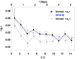
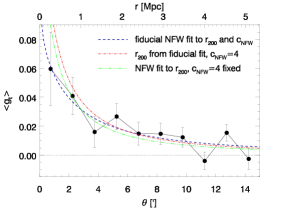
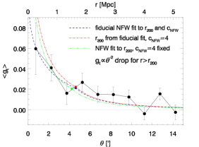
Figure 11: The tangential shear profile of CL0030+2618, averaged in bins of $90\arcsec$ width (solid line with dots). Upper panel: The best fitting NFW model in the fiducial case (see text; dashed line) and the binned cross-component $g_{\times}$ of the measured shear (dotted line with diamonds). Error bars give the standard deviation of measured values in the resp. bin. Middle panel: NFW models with $r_{200}$ from the fiducial fit and concentration set to $c_{\mathrm{NFW}}\!=\!4.0$ (dot-dashed line) and fitting to $r_{200}$ only keeping $c_{\mathrm{NFW}}\!=\!4.0$ fixed (triple dot-dashed line), compared to the fiducial fit (dashed line). Lower panel: The same models as in the middle panel, but all truncated at $r_{200}$, with a $g_{\mathrm{t}}\!\propto\theta^{-2}$ drop-off at larger radii.

6.1 The NFW model

To derive an estimator for the mass of CL0030+2618 from the weak lensing data, we fit the tangential shear profile $g_{\mathrm{t}}(\theta)$ with a NFW profile (e.g. Bartelmann 1996; Wright & Brainerd 2000). The NFW density profile has two free parameters, the radius $r_{200}$ inside which the mean density of matter exceeds the critical mass density $\rho_{\mathrm{c}}$ by a factor of $200$ and the concentration parameter $c_{\mathrm{NFW}}$ from which the characteristic overdensity $\delta_{\mathrm{c}}$ can be computed.

The overdensity radius $r_{200}$ being an estimator for the cluster’s virial radius, we define as the mass of the cluster the mass enclosed within $r_{200}$, given by:

$$M_{200}\!=\!200\frac{4\pi}{3}\rho_{\mathrm{c}}r_{200}^{3}.$$ (8)

The reduced shear observable is:

$$g_{\mathrm{NFW}}(u)\!=\!\frac{\gamma_{\mathrm{NFW}}(u)}{1-\kappa_{\mathrm{NFW}}(u)}$$ (9)

where the dimensionless radial distance $u\!=\!c_{\mathrm{NFW}}D_{\mathrm{d}}\theta r_{200}^{-1}$ contains the angular separation $\theta$ and the angular diameter distance $D_{\mathrm{d}}$ between lens and observer. The $\gamma_{\mathrm{NFW}}(u)$ and $\kappa_{\mathrm{NFW}}(u)$ profiles are given in Wright & Brainerd (2000). The critical surface mass density

$$\Sigma_{\mathrm{c}}\!=\!\frac{c^{2}}{4\pi GD_{\mathrm{d}}}\Bigg{\langle}\frac{D_{\mathrm{ds}}}{D_{\mathrm{s}}}\Bigg{\rangle}^{-1}$$ (10)

depends on $D_{\mathrm{d}}$ and the mean ratio $\langle D_{\mathrm{ds}}/D_{\mathrm{s}}\rangle$ of angular diameter distances between source and observer and source and lens.

6.2 Contamination by Cluster Galaxies

In addition to the background selection based on $g^{\prime}\!-\!r^{\prime}$ and $r^{\prime}\!-\!i^{\prime}$ colours we estimate the remaining fraction of cluster galaxies in the catalogue using the $g^{\prime}\!-\!i^{\prime}$ index. We will use this to devise a correction factor accounting for the shear dilution by (unsheared) cluster members. As discussed in Sect. B.1, the colour-magnitude diagramme of the CL0030+2618 field (Fig. 19) does not show a clear-cut cluster red sequence, but a broad distribution in $g^{\prime}\!-\!i^{\prime}$, indicating two redshift components. We therefore define a wide region $2.2\!<\!g^{\prime}\!-\!i^{\prime}\!<\!3.0$ of possible red sequence sources, including galaxies with colours similar to the $z\!=\!0.50$ CWW elliptical template but redder than the $z\!=\!0.25$ one (cf. Table LABEL:tab:galcww). As this definition of “red sequence-like” galaxies is meant to encompass all early-type cluster members, it will also contain background systems, giving an upper limit for the actual contamination in the catalogue.

Figure 10 shows the fraction of sources $2.2\!<\!g^{\prime}\!-\!i^{\prime}\!<\!3.0$ in the galaxy catalogue before (open symbols) and after (filled symbols) the final cut based on $m_{\mathrm{bright}}$ and $m_{\mathrm{faint}}$ has been applied as a function of distance to the centre of CL0030+2618 as determined by lensing (Sect. 5.2). Error bars give the propagated Poissonian uncertainties in the counts. We note a strong increase of the number of “red sequence-like” systems compared to the overall number of galaxies towards the cluster centre, indicating that a large fraction of those are indeed cluster members. Most intriguingly, the background selection seems to remove only few of these tentative cluster members, with the fractions before and after selection consistent within their mutual uncertainties at all radii. This finding can be explained to a large extent by galaxies too faint to be removed by the background selection criterion: If background selection is extended to the faintest magnitudes ($m_{\mathrm{faint}}\!=\!29$), no significant overdensity of “red sequence-like” galaxies at the position of CL0030+2618 is detected. Although using a different selection method, this modest effect of background selection is in agreement with Hoekstra (2007).

By repeating this analysis centred on several random position in our field and not finding a significant increase of the “red sequence-like” fraction towards these positions we show that the peak around the position of CL0030+2618 is indeed caused by concentration of these galaxies towards the cluster centre.

We find the residual contamination to be well represented by the sum $f_{\mathrm{cg}}(\theta)\!=\!f_{\mathrm{cg}}^{\mathrm{NFW}}(\theta)\!+\!f_{\mathrm{cg}}^{0}$ of a NFW surface mass profile and a constant (solid line in Fig. 10). We follow the approach of Hoekstra (2007) and define a radially dependent factor $f_{1}(\theta)\!=\!f_{\mathrm{cg}}^{\mathrm{NFW}}(\theta)\!+\!1$ correcting for the residual contamination. Here we take into account only the NFW component $f_{\mathrm{cg}}^{\mathrm{NFW}}(\theta)$ of the fit, as the offset $f_{\mathrm{cg}}^{0}$ represents a population of field galaxies, and not diluting cluster members. This correction factor scales up the shear estimates close to the cluster centre, counterweighing the dilution by the larger number of cluster members there.

6.3 Mass Modelling of CL0030+2618

6.3.1 Fits to the Ellipticity Profile

Table 5: Properties of the fiducial model combining the parameter values and assumptions going into the NFW modelling.

Parameter	Value	see Sect.
$\max(|\varepsilon|)$	$0.8$	4.6
$\min(\nu)$	$4.5$	4.6
$\min(\operatorname{tr}\@tens{P}^{\mathrm{g}})$	$0.1$	4.6
$m_{\mathrm{bright}}$	$20.0$	B.2
$m_{\mathrm{faint}}$	$22.5$	B.2
centre	from $S$-statistics	5.2
radial fit range	$0\arcmin\!<\!\theta\!<\!15\arcmin$	6.3.1
$f_{0}$	$1.08\pm 0.05$	4.6
$f_{1}(\theta)$	$f_{\mathrm{cg}}^{\mathrm{NFW}}(\theta)+1$	6.2
$\langle D_{\mathrm{ds}}/D_{\mathrm{s}}\rangle$	$0.33\pm 0.03$	B.3.2

In Fig. 11, there is a discernible positive tangential alignment signal extending out to $\sim\!\!10\arcmin$ or $\sim\!\!3.5\,\mbox{Mpc}$) from the cluster centre. (The solid line and dots in all panels give the shear averaged in bins of $90\arcsec$ width.) In order to validate that this tangential alignment is indeed caused by gravitational shear of a cluster-like halo, we fit the NFW reduced shear profile given in Eq. (9) to the measured shear estimates, probing the range $0\arcmin\!<\!\theta\!<\!15\arcmin$.

We define a fiducial model using the preferred parameter values presented in Table 5. The table also lists references to the sections where these values are justified. In order to determine $r_{200}$ and $c_{\mathrm{NFW}}$, we fit an NFW model to the shear estimates of the lensing catalogue galaxies, defined by the parameters above the vertical line in Table 5. Parameters below the line do not affect the catalogue but influence the relation between shear and cluster mass.

The fitting is done by minimising $\chi^{2}$ using an IDL implementation of the Levenberg-Marquardt algorithm (Moré 1978; Markwardt 2009) and returning $r_{200}^{\mathrm{fit}}\!=\!1.64\!\pm\!0.16\,\mbox{Mpc}$ and $c_{\mathrm{NFW}}^{\mathrm{fit}}\!=\!2.1\!\pm\!1.1$ for the free parameters of the model. Comparing the best-fitting NFW model (dashed curve in the upper and middle panels of Fig. 11) to the data, we find the shear profile to be reasonably well-modelled by an NFW profile: we measure $\chi^{2}/\nu_{\mathrm{dof}}\!=\!13404/13636\!\approx\!0.98$, assuming an error

$$\sigma_{\mathrm{fit}}\!=\!f_{1}(\theta)\sigma_{\mathrm{gt}}\quad,\quad\sigma_{\mathrm{gt}}\!=\!f_{0}\sigma_{\varepsilon}/\!\sqrt{2}\!\approx\!0.29$$ (11)

for the individual shear estimate. This overall agreement with NFW is consistent with shear profiles of clusters with comparable redshift and data quality (Clowe et al. 2006). We discuss the NFW parameter values obtained by the fit and the radial range over which the NFW fit is valid (the middle and lower panels of Fig. 11) in Sect. 6.

Gravitational lensing by a single axially symmetric deflector causes tangential alignment of the resulting ellipticities. Thus, the ellipticity cross-component $g_{\times}\!=\!\langle e_{\times}(\theta)\rangle$ corresponding to a pure curl field around the centre should be consistent with zero at all $\theta$. The dotted line and diamonds in the upper panel of Figure 11 show that $g_{\times}$ is indeed consistent or nearly consistent with zero in its error bars in all bins but the innermost $90\arcsec$. This feature is, like the general shapes of both $g_{\mathrm{t}}$ and $g_{\times}$, quite robust against the choice of binning. A tentative explanation for the higher $g_{\times}$ in the central bin might be additional lensing by the foreground mass concentration associated with the $z\!\approx\!0.25$ galaxies (cf. Sect. 5.1), centred to the East of CL0030+2618.

To further investigate this hypothesis, we split up the ellipticity catalogue into an eastern ($\alpha_{\mathrm{J2000}}\!>\!\alpha_{\mathrm{CL0030}}$) and western ($\alpha_{\mathrm{J2000}}\!<\!\alpha_{\mathrm{CL0030}}$) subset (with $50.0$ % of the galaxies in each) and repeat the profile fitting for both of them separately, as the influence of a possible perturber at the position of G2 should be small compared to the eastern sub-catalogue. In accordance with the mass distribution displayed in Fig. 8, in which a higher and more extended surface mass density can be found west of the centre of CL0030+2618 than east of it, the $g_{\mathrm{t}}$ signal is more significant in the sources lying to the West of the cluster than to the East. We find $r_{200,\mathrm{W}}^{\mathrm{fit}}\!=\!1.82\pm 0.22\,\mbox{Mpc}$, $c_{\mathrm{NFW,W}}^{\mathrm{fit}}\!=\!2.1\pm 1.2$, and $r_{200,\mathrm{E}}^{\mathrm{fit}}\!=\!1.47\pm 0.25\,\mbox{Mpc}$, $c_{\mathrm{NFW,E}}^{\mathrm{fit}}\!=\!1.5\pm 1.4$. The cross components in the central bins of both subsets are similarly high than in the complete catalogue with the eastern half also showing a high $g_{\times}$ in the second bin. As the values for $r_{200}$ from the two sub-catalogues are consistent given their uncertainties, we find no clear indications for a significant impact of the foreground structure. The inconspicuous lensing signal is consistent with the inconspicuous X-ray signal.

The deviation of $g_{\times}$ from zero by $\sim\!1.5\sigma$ in the central bin, out of the $10$ bins we probe, is not unexpected and does thus not pose a severe problem for the interpretation of our results with respect to $c_{\mathrm{NFW}}$ (Sect. 6.4).

In a further test, we repeated the analysis centred on G1, the brightest cluster galaxy and found very similar results in terms of shapes of $g_{\mathrm{t}}$ and $g_{\times}$ and fit parameters.

6.3.2 Likelihood analysis

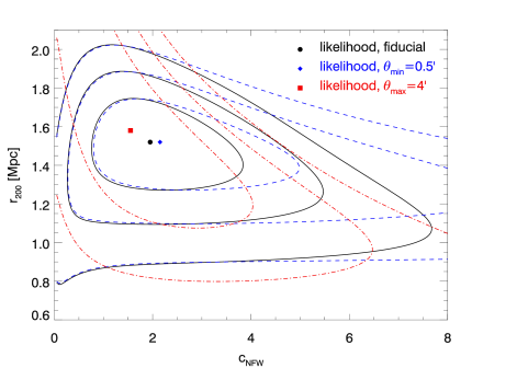
Figure 12: Confidence contours in the NFW parameter space spanned by the virial radius $r_{200}$ and concentration $c_{\mathrm{NFW}}$, corresponding to confidence levels of $99.73$%, $95.4$%, and $68.3$%. Also given as symbols are the maximum likelihood cluster parameters for three different cases. They are: the fiducial model, using data in the complete range $0\arcmin\!\leq\!\theta\!\leq\!15\arcmin$ (solid contours and dot); a model where the central $30\arcsec$ are excised from the analysis (dashed contours and diamond); and a model considering only data inside $0\arcmin\!\leq\!\theta\!\leq\!4\arcmin\!\approx\!r_{200}$ (dash-dotted contours and square).

While shear profiles serve well to investigate the agreement between a cluster shear signal and a mass distribution like NFW, there are better methods to infer model parameters, and hence the total cluster mass, than fitting techniques. Knowledge of the likelihood function

$$\mathcal{L}\!=\!\exp{\left(-\frac{1}{2}\left(\chi^{2}_{\mathrm{L}}(r_{200},c_{\mathrm{NFW}})\!-\!\chi^{2}_{\mathrm{L}}(r_{200}^{\mathrm{min}},c_{\mathrm{NFW}}^{\mathrm{min}})\right)\right)}$$ (12)

allows us to quantify the uncertainties in the model parameters given the data and – an important advantage over fitting methods – also their interdependence. We evaluate the consistency between the tangential reduced shear $g_{\mathrm{t},i}(r_{200},c_{\mathrm{NFW}})$ predicted by an NFW model for the $i$-th sample galaxy and the tangential ellipticity component $\varepsilon_{\mathrm{t},i}$ from the data by considering the function

$$\chi^{2}_{\mathrm{L}}\!=\!\sum_{i=1}^{N_{\mathrm{gal}}}{\frac{\left|g_{\mathrm{t},i}(r_{200},c_{\mathrm{NFW}})\!-\!\varepsilon_{\mathrm{t},i}\right|^{2}}{\sigma_{\mathrm{fit}}^{2}\left(1\!-\!\left|g_{\mathrm{t},i}(r_{200},c_{\mathrm{NFW}})\right|^{2}\right)^{2}}}$$ (13)

(for a derivation, see Schneider et al. 2000) which we compute for a suitable grid of test parameters $r_{200}$ and $c_{\mathrm{NFW}}$ and determine the values $r_{200}^{\mathrm{min}}$ and $c_{\mathrm{NFW}}^{\mathrm{min}}$ for which $\chi^{2}_{\mathrm{L}}$ becomes minimal. The likelihood approach also allows us to introduce a more accurate noise estimator $\sigma^{2}_{\mathrm{SKE}}\!=\!\sigma_{\mathrm{fit}}^{2}(1\!-\!|g_{\mathrm{t},i}|^{2})^{2}$ for the individual shear estimate, taking into account the dependence of the noise on the shear value itself, as expected by the model.

In Fig. 12, we present the regions corresponding to confidence intervals of $68.3$%, $95.4$%, and $99.73$% in the $r_{200}$-$c_{\mathrm{NFW}}$-parameter space for three radial ranges in which data galaxies are considered. The solid curves denote the fiducial model with the complete $0\arcmin\!\leq\!\theta\!\leq\!15\arcmin$ range, giving $r_{200}^{\mathrm{min}}\!=\!1.52^{+0.22}_{-0.24}\,\mbox{Mpc}$ and $c_{\mathrm{NFW}}^{\mathrm{min}}\!=\!2.0^{+1.8}_{-1.2}$. We will adopt these as the fiducial results of our analysis (see Table LABEL:tab:param), yielding a cluster mass of $M_{200}(r_{200}^{\mathrm{min}})\!=\!7.2^{+3.6}_{-2.9}\times 10^{14}\mathrm{M}_{\sun}$ (statistical uncertainties) by applying Eq. (8). In the following, we will discuss variations to this fiducial case (e.g. the other contours in Fig. 12).

Table 6: Parameters resulting from NFW modelling of CL0030+2618 for models relying on different assumptions.

Model	$r_{200}^{\mathrm{min}}/\mbox{Mpc}$	$c_{\mathrm{NFW}}^{\mathrm{min}}$	$M_{200}(r_{200}^{\mathrm{min}})^{\dagger}$	$\mu^{\ddagger}$
fiducial	$1.52_{-0.24}^{+0.22}$	$2.0_{-1.2}^{+1.8}$	$7.2\!\times\!10^{14}\mathrm{M}_{\sun}$	$--$
$0.5\arcmin\!\leq\!\theta\!\leq\!15\arcmin$	$1.52_{-0.24}^{+0.22}$	$2.2_{-1.4}^{+2.8}$	$7.2\!\times\!10^{14}\mathrm{M}_{\sun}$	$1.00$
$0\arcmin\!\leq\!\theta\!\leq\!4\arcmin$	$1.58_{-0.50}^{+1.85}$	$1.6_{-1.6}^{+2.4}$	$8.1\!\times\!10^{14}\mathrm{M}_{\sun}$	$1.12$
$\max(|\varepsilon|)\!=\!1.0$	$1.43_{-0.26}^{+0.24}$	$1.9_{-1.3}^{+2.0}$	$6.0\!\times\!10^{14}\mathrm{M}_{\sun}$	$0.83$
$\max(|\varepsilon|)\!=\!10^{4}$	$1.32_{-0.39}^{+0.29}$	$1.5_{-1.3}^{+2.6}$	$4.7\!\times\!10^{14}\mathrm{M}_{\sun}$	$0.65$
centred on BCG	$1.51_{-0.24}^{+0.23}$	$1.7_{-1.1}^{+1.9}$	$7.1\!\times\!10^{14}\mathrm{M}_{\sun}$	$0.98$
no contam. corr.	$1.50_{-0.24}^{+0.22}$	$1.7_{-1.0}^{+1.6}$	$7.0\!\times\!10^{14}\mathrm{M}_{\sun}$	$0.96$
$f_{0}\!=\!0.88$	$1.41_{-0.22}^{+0.19}$	$1.9_{-1.2}^{+1.8}$	$5.8\!\times\!10^{14}\mathrm{M}_{\sun}$	$0.80$
$f_{0}\!=\!1.13$	$1.54_{-0.25}^{+0.23}$	$2.0_{-1.2}^{+1.9}$	$7.5\!\times\!10^{14}\mathrm{M}_{\sun}$	$1.04$
$\langle D_{\mathrm{ds}}/D_{\mathrm{s}}\rangle\!=\!0.30$	$1.59_{-0.25}^{+0.24}$	$2.1_{-1.3}^{+1.9}$	$8.3\!\times\!10^{14}\mathrm{M}_{\sun}$	$1.14$
$\langle D_{\mathrm{ds}}/D_{\mathrm{s}}\rangle\!=\!0.36$	$1.45_{-0.23}^{+0.21}$	$1.9_{-1.2}^{+1.8}$	$6.3\!\times\!10^{14}\mathrm{M}_{\sun}$	$0.87$

^† From Eq. (8).

^‡ Mass $\mu\!=\!M_{200}/M_{200}^{\mathrm{fid}}$ in units of the fiducial cluster mass.

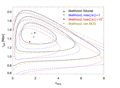
Figure 13: Confidence contours and values of $r_{200}$ and $c_{\mathrm{NFW}}$ maximising the likelihood in dependence of the maximum shear estimator $\max(|\varepsilon|)$ permitted in the catalogue: Given are the fiducial case ($\max(|\varepsilon|)\!=\!0.8$, solid contours and dot, see Sect. 4.6); $\max(|\varepsilon|)\!=\!1.0$ (dashed contours and diamond); and $\max(|\varepsilon|)\!=\!10^{4}$, equivalent to no cut (dot-dashed contours and square). Triple dot-dashed contours and the triangle denote the results for an otherwise fiducial model centred on the BCG of CL0030+2618.

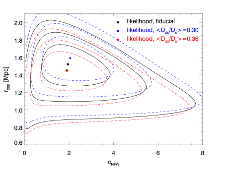
Figure 14: Confidence contours and values of $r_{200}$ and $c_{\mathrm{NFW}}$ maximising the likelihood for models of different geometric factor: The fiducial case, $\langle D_{\mathrm{ds}}/D_{\mathrm{s}}\rangle\!=\!0.33$ (solid contours and dot) is compared to the low ($\langle D_{\mathrm{ds}}/D_{\mathrm{s}}\rangle\!=\!0.30$, dashed contours and square) and high cases ($\langle D_{\mathrm{ds}}/D_{\mathrm{s}}\rangle\!=\!0.36$, dot-dashed contours and diamond) derived from the CFHTLS Deep fields in Sect. B.3.2.

6.4 The Concentration Parameter

While our resulting $r_{200}$ seems reasonable for a galaxy cluster of the redshift and X-ray luminosity of CL0030+2618, its concentration, despite the fact that it is not well constrained by our data and cluster weak lensing in general, seems low compared to the known properties of galaxy clusters:

Bullock et al. (2001) established a relation between mass and concentration parameter from numerical simulations of dark matter haloes, using a functional form from theoretical arguments:

$$c_{\mathrm{NFW}}=\frac{c_{\mathrm{NFW},0}}{1+z}\left(\frac{M_{\mathrm{vir}}}{M_{\ast}}\right)^{\alpha}$$ (14)

with $c_{\mathrm{NFW},0}=14.5\pm 6.4$ and $\alpha=-0.15\pm 0.13$ for a pivotal mass $M_{\ast}\!=\!1.3\times 10^{13}\,h^{-1}\mathrm{M}_{\sun}$. This, for $z=0.50$ and $M_{\mathrm{vir}}=7.2\times 10^{14}\,\mathrm{M}_{\sun}$ gives $c_{\mathrm{NFW}}\!=\!3.7$. Comerford & Natarajan (2007), analysing a sample of 62 galaxy clusters for which virial masses and concentration parameters have been determined, and using the same relation Eq. (14), find $c_{\mathrm{NFW},0}=9.0$ and $\alpha=-0.13$, yielding $c_{\mathrm{NFW}}=5.6_{-3.7}^{+7.3}$ for the virial mass and redshift of CL0030+2618.

This large interval is consistent within the error bars with our fiducial $c_{\mathrm{NFW}}\!=\!2.0^{+1.8}_{-1.2}$ with $\chi^{2}_{\mathrm{L}}/\nu_{\mathrm{dof}}\!=\!13413/13636$, but as the value itself remains unusually small, we investigate it further. First, we test $c_{\mathrm{NFW}}\!=\!4.0$, close to the value suggested by Bullock et al. (2001), while fixing $r_{200}^{\mathrm{fit}}\!=\!1.64\,\mbox{Mpc}$ and find $\chi^{2}_{\mathrm{L}}/\nu_{\mathrm{dof}}\!=\!13423/13637$ and the shear profile of the resulting model (dash-dotted line in the middle panel of Fig. 11) to be clearly outside the error margin for the innermost bin, demanding a significantly higher shear in the inner $90\arcsec$ than consistent with the measurements. With changes in $c_{\mathrm{NFW}}$ mainly affecting the modelling of the cluster centre, there is no such tension in the other bins. In the next step, we repeat the fit to the profile, now with $c_{\mathrm{NFW}}\!=\!4.0$ fixed and $r_{200}$ as the only free parameter. The resulting best-fitting model yields $r_{200}^{\mathrm{fit}4}\!=\!1.51\,\mbox{Mpc}$ (triple-dot dashed in the middle panel of Fig. 11), still outside but close to the measured $1\sigma$-margin of the data. As this fit gives $\chi^{2}_{\mathrm{L}}/\nu_{\mathrm{dof}}\!=\!13418/13637$, we conclude that more strongly concentrated models than the fiducial are indeed disfavoured.

Residual contamination by cluster galaxies reduces the measured concentration parameter, as can be seen when “switching off” the contamination correction factor (see Table LABEL:tab:param). This is expected as contamination suppresses the signal most strongly in the cluster centre. Removing all galaxies at separations $\theta\!<\!0.5\arcmin$ from the likelihood analysis, we indeed measure a higher $c_{\mathrm{NFW}}^{\mathrm{min}}\!=\!2.2^{+2.8}_{-1.4}$, but for the price of larger error bars, as the same galaxies close to the cluster centre have the highest constraining power on $c_{\mathrm{NFW}}$. As can be seen from the dashed contours and the diamond in Fig. 12, excising the $\theta\!<\!0.5\arcmin$ galaxies just stretches the confidence contours towards higher $c_{\mathrm{NFW}}$, leaving $r_{200}^{\mathrm{min}}\!=\!1.52_{-0.24}^{+0.22}\,\mbox{Mpc}$, and thus the inferred cluster mass unchanged (see also Table LABEL:tab:param).

Replacing the contamination correction with a background selection down to the faintest magnitudes ($m_{\mathrm{faint}}\!=\!29$), removing a large fraction of the “red sequence-like” galaxies in Fig. 10, also yields a higher $c_{\mathrm{NFW}}^{\mathrm{fit}}\!=\!3.3\pm 1.7$ in the shear profile fit, together with a slightly larger $r_{200}^{\mathrm{fit}}\!=\!1.67\pm 0.18\,\text{Mpc}$ and a less significant detection $S(\boldsymbol{\theta}_{\mathrm{c}})\!=\!5.10$ than the fiducial case. A further possible explanation for the low $c_{\mathrm{NFW}}$ due to additional lensing by the $z\!\approx\!0.25$ foreground structure is rather unlikely (cf. Sect. 6.3.1).

6.5 The Extent of the NFW Profile

Navarro et al. (1997) designed their profile to represent the mass distribution of galaxy clusters in numerical simulations within the virial radius. Thus, as theory provides no compelling argument to use it out to larger radii, this practice has to be justified empirically.

In the lower panel of Fig. 11, we show results for a toy model profile in which the shear signal drops faster than NFW outside $r_{200}$. For simplicity, we chose the shear profile of a point mass, i.e.

$$g_{\mathrm{t,ext}}(\theta)\!=\!g_{\mathrm{t,NFW}}(\theta_{200})\left(\frac{\theta_{200}}{\theta}\right)^{2}$$ (15)

for $\theta\!>\!\theta_{200}$, the separation corresponding to $r_{200}$. As in the middle panel of Fig. 11, dashed, dot-dashed, and triple dot dashed lines denote the fit to both $r_{200}$ and $c_{\mathrm{NFW}}$, setting $c_{\mathrm{NFW}}\!=\!4.0$ for the same $r_{200}$, and fitting to $r_{200}$ for a fixed $c_{\mathrm{NFW}}\!=\!4.0$, respectively. The truncation points $\theta_{200}$ are marked by squares in Fig. 11. For the usual two-parameter model with $\chi^{2}_{\mathrm{L,trunc}}\!-\!\chi^{2}_{\mathrm{L,NFW}}\!=\!0.80$, as for the other two models the truncated, the difference in goodness-of-fit between the truncated and pure NFW profiles is marginal.

Secondly, we repeat the likelihood analysis for galaxies $0\arcmin\!\leq\!\theta\!\leq\!4\arcmin\!\approx\!\theta_{200}$ only. The dash-dotted contours and the square in Fig. 12 for the resulting optimal parameters show the corresponding values. Here, $r_{200}^{\mathrm{min}}\!=\!1.58_{-0.50}^{+1.85}\,\mbox{Mpc}$ and $c_{\mathrm{NFW}}^{\mathrm{min}}\!=\!1.6^{+2.4}_{-1.6}$ are more degenerate than in the fiducial case (cf. Table LABEL:tab:param). We conclude that there is no evidence in the CL0030+2618 data for a deviation of the shear profile from NFW at $r\!>\!r_{200}$. Applying Occam’s razor, we use this profile for the whole radial range, but stress cautiously that we cannot preclude an underestimation of the errors and, to a lesser extent, a bias in the virial mass here.

6.6 Shear Calibration

As already pointed out in Sect. 4.6, the maximum shear estimator $\max(|\varepsilon|)$ considered in the catalogue strongly affects averaged shear observables. In Fig. 13, we quantify this dependence by comparing the confidence contours and best values for $r_{200}$ and $c_{\mathrm{NFW}}$ from the fiducial $\max(|\varepsilon|)\!=\!0.8$ catalogue (solid contours and dot) to cases with $\max(|\varepsilon|)\!=\!1.0$ (dashed contours and diamond) and $\max(|\varepsilon|)\!=\!10^{4}$ (dot-dashed contours and square). The latter includes even the most extreme shear estimates. The $\max(|\varepsilon|)$ cut, via the amplitude of the shear signal, mainly influences $r_{200}^{\mathrm{min}}$, reducing it by $6$ % ($13$ %) for the frequently used $\max(|\varepsilon|)\!=\!1.0$ and the extreme $\max(|\varepsilon|)\!=\!10^{4}$, respectively. In turn, the mass estimate would be reduced by $17$ % ($35$ %), as can be seen from Table LABEL:tab:param.

The influence on the mass estimate by the choice of $\max(|\varepsilon|)$ is compensated by the shear calibration $f_{0}\!\neq\!1$ and one of the effects which we account by considering different $f_{0}$. Given the uncertainty $\sigma_{\mathrm{f}_{0}}\!=\!0.05$ (Sect. 4.6), we repeat the likelihood analysis with $f_{0}\!=\!1.13$. For the negative sign, the signal dilution by foreground galaxies has to be taken into account. Combining in quadrature the $18$ % foreground dilution estimated from the CFHTLS D1 field (Sect. B.3.1) with $\sigma_{\mathrm{f}_{0}}$, we arrive at $f_{0}\!=\!0.88$ as the lower bound of the error margin. The $+5$ % ($-20$ %) variation in $f_{0}$ translates into $+1.3$ % ($-7.2$ %) in $r_{200}^{\mathrm{min}}$, yielding again $\approx\!+4$ % ($\approx\!-20$ %) variation in $M_{200}$ (see Table LABEL:tab:param).

6.7 Combined Mass Error Budget

Replacing the weak lensing centre in our fiducial model by the cluster’s BCG as the centre of the NFW profile, we find the resulting differences in $r_{200}^{\mathrm{min}}$ and $c_{\mathrm{NFW}}^{\mathrm{min}}$ returned by the likelihood method, and hence in $M_{200}$, to be small (cf. triple dot-dashed contours and triangle in Fig 13; Table LABEL:tab:param). We conclude the error on the chosen centre to be subdominant.

Variations in the geometric factor $\langle D_{\mathrm{ds}}/D_{\mathrm{s}}\rangle$ induce a similar scaling in $r_{200}^{\mathrm{min}}$ and $c_{\mathrm{NFW}}^{\mathrm{min}}$ as shear calibration does. Using the error margin from the determination of the distance ratios from the CFHTLS Deep fields (Sect. B.3.2), we produce likelihood contours for $\langle D_{\mathrm{ds}}/D_{\mathrm{s}}\rangle\!=\!0.30$ (dashed lines and square in Fig. 14) and $\langle D_{\mathrm{ds}}/D_{\mathrm{s}}\rangle\!=\!0.36$ (dot-dashed contours and diamond). Comparing to the fiducial model (solid contours and dot), we find an increase in $r_{200}^{\mathrm{min}}$ by $4.6$ % and by $14$ % in $M_{200}$ for $\langle D_{\mathrm{ds}}/D_{\mathrm{s}}\rangle\!=\!0.30$ (a more massive lens is needed for the same shear if the source galaxies are closer on average) and a decrease by $4.6$ % in $r_{200}^{\mathrm{min}}$ and $13$ % in $M_{200}$ for $\langle D_{\mathrm{ds}}/D_{\mathrm{s}}\rangle\!=\!0.36$ (cf. Table LABEL:tab:param).

An additional source of uncertainty in the mass estimate not discussed so far are triaxiality of galaxy cluster dark matter haloes and projection of the large-scale structure (LSS) onto the image. King & Corless (2007) and Corless & King (2007) showed with simulated clusters that masses of prolate haloes tend to get their masses overestimated in weak lensing while masses of oblate haloes are underestimated.

Again owing to cosmological simulations, Kasun & Evrard (2005) devised a fitting formula for the largest-to-smallest axis ratio $\eta$ of a triaxial haloes as a function of redshift and mass

$$\eta(M_{200},z)\!=\!\eta_{0}(1+z)^{\epsilon}\left(1-\zeta\ln\left(\frac{M_{200}}{h\,10^{15}\,\mathrm{M}_{\sun}}\right)\right)$$ (16)

with $\epsilon\!=\!0.086$, $\zeta\!=\!0.023$, and $\eta_{0}\!=\!0.633$. Inserting the values for CL0030+2618, we find $\eta\!=\!0.61$ and, like Dietrich et al. (2009) whose lines we are following, derive the following maximal biases from Corless & King (2007): for a complete alignment of the major cluster axis with the line of sight mass is overestimated by $16$ %, while complete alignment with the minor axis results in a $10$ % underestimation.

The projection of physically unrelated large scale structure can lead to a significant underestimation of the statistical errors in $M_{200}$ and $c_{\mathrm{NFW}}$ (Hoekstra 2003, 2007). The simulations of Hoekstra (2003) yield an additional error of $\pm 1.2\,h^{-1}\!\times\!10^{14}\mathrm{M}_{\sun}\!=\!\pm 1.67\times 10^{14}\mathrm{M}_{\sun}$ for a cluster in the mass range of CL0030+2618, and little redshift dependence for $z\!>\!0.2$. Thus, we adopt this value as the systematic uncertainty due to large scale structure.

We define the systematice mass uncertainty $\sigma_{\mathrm{sys}}$ as the quadratic sum of the errors $\sigma_{\mathrm{cali}}$ from shear calibration, $\sigma_{\mathrm{geom}}$ from the geometric factor, $\sigma_{\mathrm{proj}}$ from projection, and $\sigma_{\mathrm{LSS}}$ from large-scale structure. The total error, used in Fig. 15, is then defined as the quadratic sum also including $\sigma_{\mathrm{stat}}$:

$$\sigma_{\mathrm{tot}}^{2}=\sigma_{\mathrm{stat}}^{2}\!+\!\sigma_{\mathrm{sys}}^{2}=\sigma_{\mathrm{stat}}^{2}\!+\!\sigma_{\mathrm{LSS}}^{2}\!+\!\sigma_{\mathrm{proj}}^{2}\!+\!\sigma_{\mathrm{geom}}^{2}\!+\!\sigma_{\mathrm{cali}}^{2}$$ (17)

We note that the statistical errors are already quite large and the dominating factor in Eq. (17). As its main result, this study arrives at a mass estimate of $M_{200}\!=\!7.2^{+3.6+2.3}_{-2.9-2.5}\times 10^{14}\mathrm{M}_{\sun}$ for CL0030+2618, quoting separately the statistical and systematic error as the first and second uncertainty.

6.8 Comparison to X-ray masses

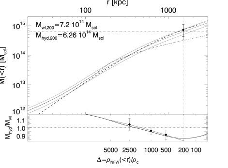
Figure 15: Comparison of mass profiles of CL0030+2618.
Upper panel: The hydrostatic mass $M_{\mathrm{hyd}}(<\!r)$ derived from the Chandra analysis (thick solid line). A constant ICM temperature is assumed and the grey lines delineate the error margin derived from its error. The dash-dotted line gives the Chandra profile for a more realistic temperature profile. The dot with error bars and the dashed line denote the mass estimate and profile $M_{\mathrm{wl}}(<\!r)$ from our weak lensing analysis, assuming an NFW profile. The thick error bars show the statistical errors while thin bars include all components dicussed in Sect. 6.7. Lower panel: Ratio of X-ray to lensing mass as a function of radius (black line). The symbols and grey line show the $M_{\mathrm{hyd}}/M_{\mathrm{wl}}$ found by Zhang et al. (2010) at three overdensity radii and their fitted relation.

We will now compare this weak lensing mass to a mass profile drawn from the Chandra analysis of CL0030+2618. Under the assumption that the ICM is in hydrostatic equilibrium, the total mass $M(<\!r)$ of a galaxy cluster within a radius $r$ can be derived as (cf. Sarazin 1988):

$$M(<\!r)\!=\!\frac{-k_{\mathrm{B}}T_{\mathrm{X}}(r)r}{\mu m_{\mathrm{p}}G}\left(\frac{\mathrm{d}\ln\rho_{\mathrm{g}}}{\mathrm{d}\ln r}+\frac{\mathrm{d}\ln T_{\mathrm{X}}}{\mathrm{d}\ln r}\right)$$ (18)

where $m_{\mathrm{p}}$ is the proton mass and $\mu$ the mean molecular mass. In a first step, we treat the ICM temperature to be independent of the radius and fix it to the Vikhlinin et al. (2009a) value of $k_{\mathrm{B}}\langle T_{\mathrm{X}}\rangle\!=\!5.63\pm 1.13\,\mbox{keV}$. For the gas density $\rho_{\mathrm{g}}$, we use a (simplified) Vikhlinin et al. (2006) particle density profile

$$\sqrt{n_{\mathrm{e}}n_{\mathrm{p}}}\!=\!n_{0}^{2}\frac{\left(r/r_{\mathrm{c}}\right)^{-\alpha}}{\left(1+r^{2}/r_{\mathrm{c}}^{2}\right)^{3\beta-\alpha/2}}\frac{1}{\left(1+r^{\gamma}/r_{\mathrm{s}}^{\gamma}\right)^{\varepsilon/\gamma}}$$ (19)

Table 7: Parameters and fit values of the Vikhlinin et al. (2006) ICM model for CL0030+2618.

Parameter	Quantity	Fit Value
$n_{0}^{2}$	pivot density	$3.784\times 10^{-3}\,\mbox{cm}^{-3}$
$r_{\mathrm{c}}$	core radius	$139\,\mbox{kpc}$
$r_{\mathrm{s}}$	scale radius	$421\,\mbox{kpc}$
$\alpha$	exponent	$0.5867$
$\beta$	exponent	$0.4653$
$\varepsilon$	exponent	$1.2293$

with the parameters given in Table 7 and a fixed $\gamma\!=\!3$ and arrive at a mass of $M_{\mathrm{hyd}}\!=\!(6.26\pm 1.26)\times 10^{14}\,\mathrm{M}_{\sun}$ at the virial radius of $r_{200}\!=\!1.52\,\mbox{Mpc}$ obtained in the lensing analysis. We show the corresponding mass profile as the thick and its error margin as the grey lines in the upper panel of Fig. 15.

This value is in very good agreement with the weak lensing mass estimate (dot with thick error bars for statistical and thin error bars for systematic plus statistical uncertainties in Fig. 15). The consistency between the X-ray mass profile derived from $T_{\mathrm{X}}$ and the (baryonic) ICM using Eq. 19 and the NFW profile describing the combined dark and luminous matter densities holds at all relevant radii $\gtrsim\!50\,\mbox{kpc}$ in a wide range from the cluster core till beyond the virial radius.

Assuming an isothermal cluster profile, one likely overestimates the total hydrostatic mass, as the ICM temperature is lower at the large radii dominating the mass estimation around $r_{\mathrm{vir}}$. The competing effect of the temperature gradient term in the hydrostatic equation is subdominant compared to this effect of the temperature value.

Therefore, to estimate the systematic uncertainty arising from isothermality, we consider a toy model temperature profile consisting of the flat core at $\langle T_{\mathrm{X}}\rangle$, an power-law decrease at larger radii, and a minimal temperature $k_{\mathrm{B}}T_{0}\!=\!0.5\,\mbox{keV}$ in the cluster outskirts to qualitatively represent the features of an ensemble-averaged temperature profile:

$$k_{\mathrm{B}}T_{\mathrm{X}}(r)\!=\!\begin{cases}k_{\mathrm{B}}\langle T_{X}\rangle&r\!\leq\!r_{\mathrm{i}}\\ p\,r^{q}&r_{\mathrm{i}}\!\leq\!r\!\leq\!r_{\mathrm{t}}\\ k_{\mathrm{B}}T_{0}&r\!\geq\!r_{\mathrm{t}}\end{cases}$$ (20)

where we choose a core radius $r_{\mathrm{i}}\!=\!r_{200}/8$ (as used in Pratt et al. 2007), a power-law slope $q\!=\!-0.4$ taken as a typical value found by Eckmiller et al. (in prep.), and fixing the truncation radius $r_{\mathrm{t}}$ and amplitude $p$ demanding continuity of $T_{\mathrm{X}}(r)$. The mass profile resulting from this temperature distribution is plotted in Fig. 15 (upper panel) as the dash-dotted line, giving an estimate of the systematic uncertainty in the X-ray profile. Its value coincides with the lower end of the $1\sigma$ mass range for $M_{\mathrm{wl}}$ at $r_{200}$, taking into account its systematic errors. Another systematic factor in X-ray analysis is non-thermal pressure support, leading to an underestimation of the X-ray mass by $\sim\!10$ % (e.g. Zhang et al. 2008). Taking into account all these effects, we conclude a very good agreement of X-ray and weak lensing mass estimates of CL0030+2618, despite the potential perturbation by the line-of-sight structure.

In the lower panel of Fig. 15, we show the ratio $M_{\mathrm{hyd}}/M_{\mathrm{wl}}$ of hydrostatic X-ray and weak lensing mass as a function of radius. Although this quantity has a large error, our values are in good agreement with the X-ray-to-lensing mass ratios found by Zhang et al. (2010) for a sample of relaxed clusters for three radii corresponding to overdensities $\Delta\!=\!\rho_{\mathrm{NFW}}(<\!r)/\rho_{\mathrm{c}}\!=\!2500$, $1000$, and $500$ (black line). We note that we recover well the relation $\frac{M_{\mathrm{hyd}}}{M_{\mathrm{wl}}}(\Delta)$ found by Zhang et al. (2010) by fitting their cluster sample data (grey line).

7 Summary and Conclusion

With this study, we report the first results for the largest weak lensing survey of X-ray selected, high-redshift clusters, the 400d cosmological sample defined by Vikhlinin et al. (2009a) and determine a weak lensing mass for an interesting cluster of galaxies, CL0030+2618, which had not been studied with deep optical observations before. We observed CL0030+2618, along with other clusters of our sample, using the Megacam $\sim\!24\arcmin\times 24\arcmin$ imager at the MMT, obtaining deep $g^{\prime}r^{\prime}i^{\prime}$ exposures. Employing an adaptation of the Erben et al. (2005) pipeline, THELI, and the “TS” KSB shape measurement pipeline presented by T. Schrabback in Heymans et al. (2006), we, for the first time, measure weak gravitational shear with Megacam, showing its PSF properties to be well suited for such venture.

The lensing catalogue of background galaxies is selected by a photometric method, using $g^{\prime}r^{\prime}i^{\prime}$ colour information. Despite similar number count statistics, we find different photometric properties in our Megacam field than in the CFHTLS Deep fields used to estimate the redshift distribution of the lensed galaxies. The photometric measurements establish the galaxy we name G1, for which Boyle et al. (1997) determined a redshift $z\!=\!0.516$ as the BCG of CL0030+2618, ruling out a slightly brighter source found inconsistent in its colours with the cluster redshift $z\!=\!0.50$. We find additional evidence for the presence of a foreground structure at $z\!\approx\!0.25$ from photometry but find it does neither significantly affect the lensing nor the X-ray mass estimate of CL0030+2618.

Having applied several consistency checks to the lensing catalogue and optimising the aperture mass map of the cluster, we detect CL0030+2618 at $5.84\sigma$ significance. The weak lensing centre obtained by bootstrapping this map is in good agreement with the BCG position and the X-ray detections by Rosat, Chandra, and XMM-Newton. Two tentative strong lensing arcs are detected in CL0030+2618.

Tangential alignment of galactic ellipticities is found to extend out to $10\arcmin$ separation and well modelled by an NFW profile out to $>\!2r_{200}$. The low concentration parameter found by least-squares fitting to the shear profile is confirmed by the likelihood method with which we determine CL0030+2618 to be parametrised by $r_{200}^{\mathrm{min}}\!=\!1.52^{+0.22}_{-0.24}\,\mbox{Mpc}$ and $c_{\mathrm{NFW}}^{\mathrm{min}}\!=\!2.0^{+1.8}_{-1.2}$. Modifying the likelihood analysis for the fiducial case, we estimate systematic errors due to shear calibration, the redshift distribution of the background galaxies, and the likely non-sphericity of the cluster. Further, we confirm the best model to change little if the BCG is chosen as cluster centre rather than the weak lensing centre. We arrive at a virial weak lensing mass for CL0030+2618 with statistical and systematic uncertainties of $M_{200}\!=\!7.2^{+3.6+2.3}_{-2.9-2.5}\times 10^{14}\mathrm{M}_{\sun}$, in excellent agreement with the virial mass obtained using Chandra and the hydrostatic equation, $M_{\mathrm{hyd}}\!=\!6.26\pm 1.26\times 10^{14}\mathrm{M}_{\sun}$.

Noting that statistical errors on the lensing mass are still high, we conclude that high-quality data and well-calibrated analysis techniques are essential to exploit the full available cosmological information from the mass function of galaxy clusters with weak lensing. Nevertheless, once lensing masses for all the $36$ clusters in the sample are available, these statistical errors are going to be averaged out and reduced by a factor of 6 by combining all clusters when testing for cosmological parameters. Thus, understanding and controlling systematic errors remain important issues. We are going to proceed our survey with the analysis of further high-redshift clusters from the 400d cosmological sample observed with Megacam.

Appendix A Details of Data Reduction

In this Appendix, we provide a detailed view of the subtleties of the data reduction outlined in Sect. 3.

A.1 Chips and Amplifiers

The MMT Megacam control software offers a number of options for the CCD readout. As already mentioned in Sect. 2.2, there are 36 physical CCD chips each of them is equipped with two output amplifiers, giving a readout of $1024\!\times 4608\!$ (unbinned) pixels per amplifier. For our programme, we have chosen to use all 72 amplifiers each reading out half a chip, thus reducing readout time by a factor of two. As a result, Megacam raw images are multi-extension fits files with 72 extensions.

Owing to this, all run processing tasks are performed on the 72 subframes individually. Files from the two chips of an amplifier are joined at the end of the run processing prior to the astrometric calibration in order to increase the usable surface for the astrometric procedures.

A.2 The “Run Processing” Stage

• De-biasing: By stacking all bias frames taken within a suitable time interval around the date of science observations, a master bias image is constructed and subtracted from all other frames.

• Flatfielding: THELI applies a two-step process. First, science frames are divided by a master sky flatfield frame. In the second step, the median of all science frames is calculated, discarding the positions at which objects have been detected by SExtractor (Bertin & Arnouts 1996). Due to the dithering, for every pixel in the field-of-view, these “superflats” contain signal from the sky background from slightly different positions on the sky. Thus, the superflat provides a measure to compare the response in different pixels.

  Selecting the frames to contribute into the superflat to achieve the optimal flatness of the background is the most time-consuming and work-intensive step in run processing, as inhomogeneities in individual frames will propagate into the superflat. Imperfect photometric conditions and variable instrumental gains are two common reasons for science frames to be removed from the calculation of the superflat. Very bright stars near target clusters, e.g. HIP 9272 (BD -00 301) with $V\!=\!8.28$ at $2\arcmin$ distance from CL0159+0030, exacerbate the situation. Involving many iterations of the – manual – frame selection process, our superflatfielding is effective in reducing the relative background variation over the field in the superflatfielded exposures to $<\!1.5$ %, and to $<\!1.0$ % for most exposures.

  In the superflatfielding stage, the different sensitivities of the amplifiers are determined and equalised, taking into account all exposures within the THELI run. This we can do, because the relative sensitivities of most of the amplifiers are constant most of the time. Gain equalisation is achieved by scaling each amplifier with an appropriate factor detailed in Erben et al. (2005, Sect. 4.7). Some amplifiers, however, experience gain fluctuation on short timescales of the order of days. In such situation the same superflatfield frame can no longer provide the same quality of flattening to all exposures such that we had to split the $g^{\prime}$-band data taken on Nov. 8, 2005 from the rest of the exposures taken on Oct. 30, 2005 and Nov. 1, 2005, at the cost of a lower number of exposures contributing to the superflatfield in each of the two sub-runs.

• De-fringing: In the bands where this is necessary, the fringing pattern can be isolated from the high spatial frequencies of the superflat and subtracted from the science frames. On the other hand, we divide by the superflat containing the lower spatial frequencies which carry information about the (multiplicative) “flatfield” effects.

• Satellite tracks: We identify satellite tracks by visual inspection when assessing frames for superflat construction and mask pixels which are affected in the given exposure. Masked pixels (stored as a DS9 region files) are set to zero in the construction of the weight images.

• Weight images: Taking into account bad pixel information from the bias, flatfield, and superflatfield frames we construct a weight image, i.e. noise map, for each individual amplifier and exposure in the run. Our algorithm is not only sensitive to cold and hot pixels but also to charge “bleeding” in the vicinity of grossly overexposed stars.

A.3 The “Set Processing” Stage

Figure 16: Mean stellar anisotropies $\langle e_{1,2}\rangle$ found in the r’-band frames of CL0030+2618 fulfilling the seeing condition $s<1.0\arcsec$. All images with $\langle\left|e\right|\rangle<0.05$ are included in the final coaddition (inner circle), while those exceeding $\langle\left|e\right|\rangle<0.06$ (outer circle) are always rejected. The decision for intermediary objects (see below) is based on visual inspection.

Figure 17: Spatial distribution of stellar anisotropies for an example exposure of high overall PSF anisotropy. Shown are the sizes and orientations of the raw ellipticity $e$ for stars identified in the MMT Megacam exposures of CL0030+2618 labelled 0936 (upper panel) and 0952 (lower panel) in Fig. 16. While within each chip the $x$ and $y$ pixel axes are to scale the array layout is only schematic.

Table 8: Coefficients of photometric calibration defined by Eq. (4) for the photometric nights used to calibrate the observations of CL0030+2618, CL0159+0030, and CL0809+2811.

Filter	Obs. Date	$Z_{\mathrm{f}}^{\dagger}$	$\beta_{\mathrm{f}}$	colour index	$\gamma_{\mathrm{f}}$	$n_{\mathrm{par}}^{\ddagger}$
$g^{\prime}$	2005-10-30	$27.27\pm 0.02$	$0.106\pm 0.007$	$g^{\prime}\!-\!r^{\prime}$	$-0.14\pm 0.02$	3
	2005-10-31	$27.15\pm 0.02$	$0.124\pm 0.008$	$g^{\prime}\!-\!r^{\prime}$	$-0.08\pm 0.01$	3
	2005-11-01	$27.35\pm 0.02$	$0.115\pm 0.005$	$g^{\prime}\!-\!r^{\prime}$	$-0.21\pm 0.02$	3
$i^{\prime}$	2005-10-30	$26.49\pm 0.02$	$0.127\pm 0.004$	$r^{\prime}\!-\!i^{\prime}$	$-0.11\pm 0.02$	3
	2005-10-31	$26.47\pm 0.01$	$0.122\pm 0.002$	$r^{\prime}\!-\!i^{\prime}$	$-0.09\pm 0.01$	3
	2005-11-01	$27.41\pm 0.01$	$0.119\pm 0.002$	$r^{\prime}\!-\!i^{\prime}$	$-0.03\pm 0.01$	3
$r^{\prime}$	2005-10-30	$26.95\pm 0.02$	$0.046\pm 0.002$	$g^{\prime}\!-\!i^{\prime}$	$-0.10\pm 0.02$	3
	2005-10-31	$26.90\pm 0.01$	$0.043\pm 0.003$	$g^{\prime}\!-\!i^{\prime}$	$-0.05\pm 0.01$	3
	2005-11-01	$26.96\pm 0.01$	$0.048\pm 0.004$	$g^{\prime}\!-\!i^{\prime}$	$(-0.10)^{\S}$	2
	2005-11-08	$26.81\pm 0.01$	$0.046\pm 0.003$	$g^{\prime}\!-\!i^{\prime}$	$(-0.10)^{\S}$	2

^† Normalised to an exposure time of $1\mbox{s}$ and an airmass $a\!=\!0$.

^‡ Number of parameters used in the fit.

^§ Fixed to default value.

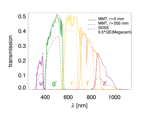
Figure 18: Comparison of the SDSS and Megacam filter systems. The plot shows the complete transmission curves for the $u^{\prime}g^{\prime}r^{\prime}i^{\prime}z^{\prime}$ filters of both systems as a function of wavelength, including the atmospheric transmissivity (as given for the SDSS site), the CCD quantum efficiency, and the actual effect of the filter, as measured in the laboratory. The solid lines give sensitivities of Megacam filters for photons incident on the optical axis while the dash-dotted lines show the same quantity near the corner of the Megacam array. Overplotted as dashed lines are the transmission curves defining the SDSS bandpass system. The black, dotted curve shows the Megacam quantum efficiency we derive from the instrument specifications, scaled by one half to show it conveniently on the plot. Note that we need to interpolate its values from only five points in the range $300\leavevmode\nobreak\ \text{nm}\!<\!\lambda\!<\!1000\leavevmode\nobreak\ \text{nm}$ and have to extrapolate outside it.

• Astrometry: We perform the astrometric calibration of our data using the best available catalogue as a reference. In case of overlap with SDSS Data Release Six (Adelman-McCarthy et al. 2008) this is the SDSS catalogue; otherwise we employ the shallower USNO B1 catalogue (Monet et al. 2003), as it is the densest all sky astrometric catalogue. The astrometric calibration is carried out by the TERAPIX software Scamp (Bertin 2006), replacing the Astrometrix programme earlier used within THELI. We find Scamp to be more robust than Astrometrix when working on chips with a small field-of-view on the sky, as given for Megacam (see Sect. 3). Compared to the otherwise similar design of MegaPrime/MegaCam at the Canada-France-Hawaii Telescope the MMT Megacam chips cover $\sim\!1/6$ of the solid angle on the sky, reducing the number of usable sources for astrometry by a similar factor leading to less accurate and robust astrometric solutions in case these are calculated on a chip-to-chip basis.

  The most important innovation is, that while Astrometrix determines an astrometric solution for each chip (Megacam amplifier in our case) individually, Scamp recognises the amplifiers of one exposure belonging together and can take into account information on the array configuration, drastically reducing the effort to be invested into this task.

  We provide these additional constraints by defining a template for the same instrument configuration and filter. This template is drawn from the observation of a dense field, i.e. a star cluster. This template guarantees a sensible solution even with few ($\lesssim\!20$) astrometric standard stars per chip, a condition frequently met with Megacam in poor fields.

  Furthermore, by running Scamp on all frames in all filters for a given target cluster with only one call to the software, we ensure consistency of the astrometric solutions among the THELI sets corresponding to the resulting stacks in different passbands.

  For the combined data set of CL0030+2618, we achieve an accurate calibration with a $1\sigma$ intrinsic accuracy of $0\aas@@fstack{\prime\prime}04$ of the sources detected with Megacam and $0\aas@@fstack{\prime\prime}27$ with respect to the astrometric standard catalogue USNO B1.

• Relative photometry: Simultaneously with the astrometric calibration, the relative photometric zeropoints of the frames are established by Scamp. In the first part of this two-step process, relative zeropoints are determined only from the differences in flux found for the astrometric reference stars in different exposures. These are independent from the absolute photometric calibration detailed in Sect. 3.2.

  In this first step, fluxes of the same object in different exposures are compared. For the coadded image resulting from stacking to be well-calibrated, the variation in relative zeropoints among the contributing frames needs to be small. We decide to include only images which show a zeropoint less than 0.1 magnitudes from the median zeropoint:

  $$Z_{\mathrm{rel}}\!-\!\operatorname{median}(Z_{\mathrm{rel}})\!<\!-0.1$$ (21)

  In the second step, if the absolute photometric calibration (Sect. 3.2) has been applied already, we compute the corrected zeropoints defined in Hildebrandt et al. (2006, Eq. (2)) of those individual frames we consider to be taken under photometric conditions. As detailed in Hildebrandt et al. (2006), corrected zeropoints are a useful consistency check, as they are the same for exposures obtained in photometric conditions.

• Coaddition: Conforming with THELI standard, SWarp is used to stack (“coadd”) images. This, together with the Scamp astrometry, also removes optical distortions, yielding a constant pixel scale in the coadded image. The final products of the set stage are the coadded image and the corresponding weight image (Fig. 2).

A.4 Image Selection

The success of a lensing analysis crucially depends on the data quality. Because of the necessity to establish a common image coordinate system and to rebin all data onto the new grid, the stacking process is a potential source of biases to the shape information. It is evident that the decision which frames should contribute to the shape measurement is of great importance. Apart from seeing and photometric quality which can be easily assessed while the observation takes place, PSF anisotropy is a key factor as it can only be corrected up to a certain degree.

We found that irrespective of the seeing, a significant fraction of the Megacam exposures from the observing runs in October 2004, October 2005, and January 2008, covering the four clusters CL0030+2618, CL0159+0030, CL0230+1836, and CL0809+2811 suffer from highly elliptic PSF which shows little variation over the field-of-view.

Inspecting the anisotropy stick plots like Fig. 17 for a fair fraction of all frames taken in these three above-mentioned runs, we come up with the following criterion: If the mean ellipticity in the stars is $\langle\left|e\right|\rangle\!<\!0.05$ (the smaller circle in Fig. 16) the variations over the field due to the properties of the optical system are clearly discernible. These frames do not suffer from a large tracking error and thus we include them in the analysis in any case. On the other hand, exposures whose stars are more elliptical than $\langle\left|e\right|\rangle\!>\!0.06$ (the larger circle in Fig. 16) show a stellar anisotropy which is mostly constant over the field which we can attribute to MMT tracking errors of varying strength. These frames are excluded from the lensing analysis. In the intermediary case of $0.05\!<\!\langle\left|e\right|\rangle\!<\!0.06$ we decide on a case-to-case basis by inspecting the respective anisotropy stick plot where frames in which the “tracking error-like” contributions seem prevalent are excluded.

A.5 The Megacam filter system

To establish the transformation between MMT and SDSS measurements, we need to know the transmissivities of both instruments to a great detail. For Megacam, the instrument website offers detailed laboratory transmission curves of the actual filters and a few data points on the CCD’s quantum efficiency. We average the tabulated quantum efficiency values over the 36 Megacam chips. Correspondingly, the SDSS collaboration provides data on the combined sensitivity of its camera/filter system. Assuming the atmospheric absorption to behave the same on both sites, we can directly compare the responses of the two instruments, as visualised in Fig. 18.

A.6 Results of Photometric Calibration

Photometric calibration is achieved by fitting Eq. (4) to the instrumental magnitudes of the photometric standards (Sect. 3.2.1). For each filter, we chose a colour index in Eq. (4) which has been proven a reliable transformation in calibration of the Canada-France-Hawaii Telescope Legacy Survey (CFHTLS) data which also uses a similar filter system. These colour indices are given in Table 8 which shows the results for the fit parameters $Z_{\mathrm{f}}$, $\beta_{\mathrm{f}}$, and $\gamma_{\mathrm{f}}$ for the photometric nights used to calibrate the CL0030+2618 data (i.e. the datasets for CL0030+2618, CL0159+0030, and CL0809+2811; Sect. 3.2.2).

Comparing the colour terms $\beta_{\mathrm{f}}$ for the different nights, we find considerable agreement of the values for all three bands, although the error bars from fitting Eq. (4) might underestimate the true errors. While our determinations of $\beta_{\mathrm{r}}$ are all consistent with each other, there is some tension between the $\beta_{\mathrm{g}}$ values. In previous Megacam studies, (Hartman et al. 2008, Table 5) quote $\beta_{\mathrm{g}}\!=\!0.122\pm 0.002$ and $\beta_{\mathrm{i}}\!=\!0.137\pm 0.002$, the first in agreement to our results, the latter significantly higher than our value. Furthermore, Walsh et al. (2008) find $\beta_{\mathrm{g}}\!=\!0.091\pm 0.068$, consistent with our values due to the large error bar. We suggest that the large span in values for $\beta_{\mathrm{g}}$ might be due to the dependence of the filter throughput as a function of distance to the optical axis, which is strongest an this band. Further investigation is needed to conclude about this issue.

Appendix B The Background Catalogue

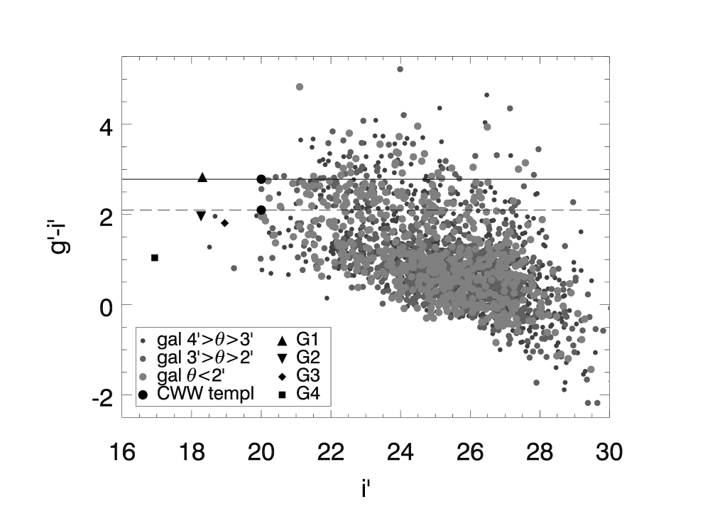
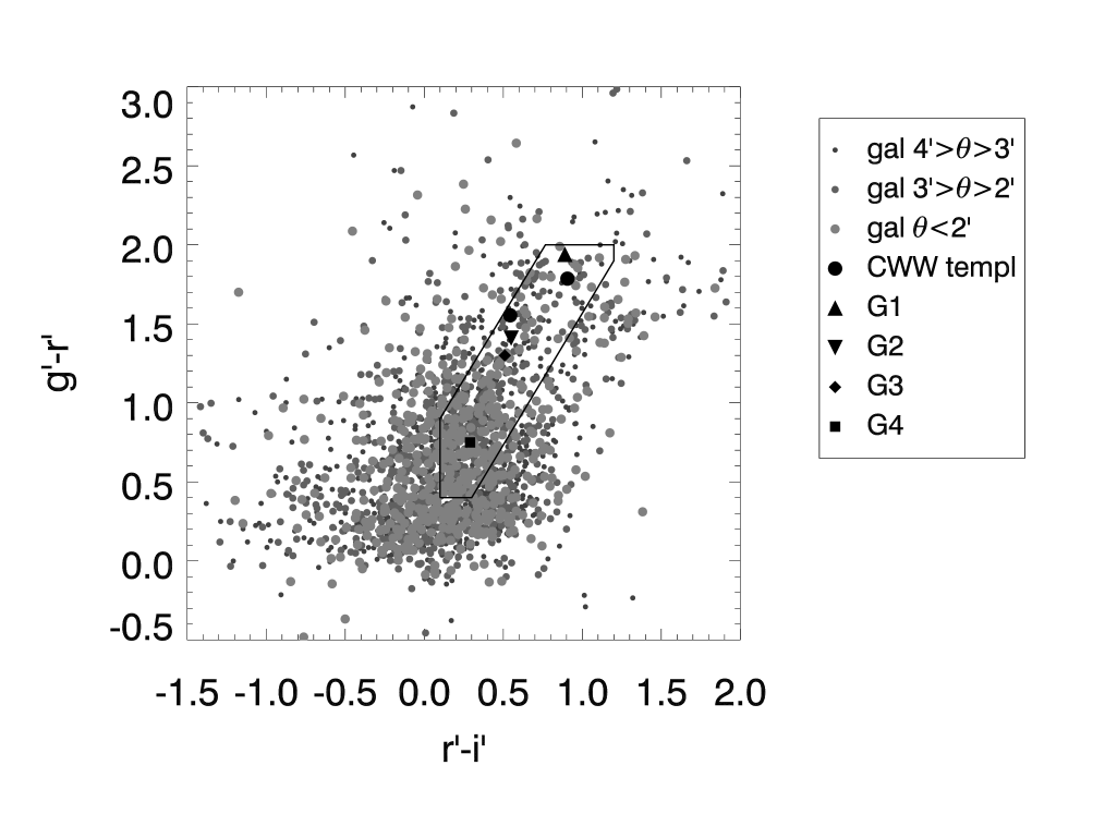
Figure 19: Upper plot: Colour-magnitude diagramme of KSB galaxies with a radial distance $\theta\!<\!4\arcmin$ from the centre of CL0030+2618. Symbol sizes and shades of grey denote galaxies from the galaxy shape catalogue in different cluster-centric radial bins. The $g^{\prime}\!-\!i^{\prime}$ colours of Coleman et al. (1980, CWW) template galaxies at $z\!=\!0.5$ (solid line and large dot at $i^{\prime}\!=\!20$) and $z\!=\!0.25$ (dashed line and large dot) are shown for comparison, as well as four notable bright galaxies detailed in Table LABEL:tab:gal. Lower plot: Colour-colour diagramme with the same objects. The polygonal region delineating the locus of bright galaxies (cf. Fig. 20) is given for comparison.

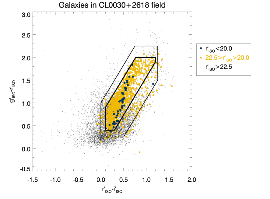
Figure 20: Colour-colour selection of the lensing catalogue: plotted are the $g^{\prime}\!-\!r^{\prime}$ vs. $r^{\prime}\!-\!i^{\prime}$ colours of the objects in the galaxy shape catalogue (with cuts on $\min{(\operatorname{tr}{\@tens{P}^{g}})}$, $\min{(\nu_{\mathrm{gal}})}$, and $\max{(\left|(\varepsilon\right|)}$ already applied). The galaxy sample is divided into three magnitude bins by the $m_{\mathrm{bright}}$ and $m_{\mathrm{faint}}$ parameters. All sources brighter than $m_{\mathrm{bright}}$ (largest dots) are removed in producing the final lensing catalogue while all sources fainter than $m_{\mathrm{faint}}$ smallest dots) are kept. Intermediately bright galaxies with $m_{\mathrm{bright}}\!<\!r^{\prime}\!<\!m_{\mathrm{faint}}$ (medium-sized dots) mark the transition between these two regimes. Only in this magnitude interval, the selection into the final galaxy catalogue by colour indices applies: sources outside the thick polygon bounding the region in which we find the brighter galaxies and likely cluster members are included in the final catalogue. See Table 9 for the definition of the polygon tracing the locus of bright galaxies.

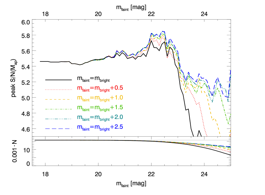
Figure 21: Upper panel: The maximum $M_{\mathrm{ap}}$ signal-to-noise ratio found in the vicinity of CL0030+2618 as a function of the background selection introduced by $m_{\mathrm{faint}}$ and $m_{\mathrm{bright}}$. The solid line corresponds to a magnitude cut $m_{\mathrm{bright}}\!=\!m_{\mathrm{faint}}$ while the dotted, dashed, dot-dashed, triple dot-dashed, and long-dashed lines denote background selections by galaxy colours in increasingly wide intervals of $m_{\mathrm{faint}}\!-\!m_{\mathrm{bright}}\!=\!\{0.5,1.0,1.5,2.0,2.5\}$ respectively. Here, the smaller polygon in Fig. 20 is used, assuming a well-defined locus of cluster galaxies in colour-colour-space and, in turn, for a rather inclusive selection of galaxies. Lower panel: The number $N$ of galaxies in the shear catalogue as a function of $m_{\mathrm{bright}}$ and $m_{\mathrm{faint}}$. The horizontal line gives $N\!\approx\!16000$ before applying any background selection for comparison. The colours and line-styles denote the same cases as in the upper panel.

Table 9: Tested regions in colour-colour space inside which galaxies with $m_{\mathrm{bright}}\!<\!r^{\prime}\!<\!m_{\mathrm{faint}}$ are excised from the lensing catalogue.

Polygon	$\min{(r^{\prime}\!-\!i^{\prime})}$	$\max{(r^{\prime}\!-\!i^{\prime})}$	$\min{(g^{\prime}\!-\!r^{\prime})}$	$\max{(g^{\prime}\!-\!r^{\prime})}$	$\min{(s)}$	$\max{(s)}$
large	0	1.25	0.25	2.25	-1.0	0.583
small	0.1	1.2	0.4	2.0	-0.733	0.1

B.1 Photometric Analysis: The Red Sequence

In clusters of galaxies at low and moderate redshifts, early-type galaxies, i.e. elliptical and spheroidal systems tend to be more common than disk galaxies. Cluster galaxies are observed to be deficient in gas and thus show little ongoing star formation but are on average dominated by old, red stellar populations (e.g., Bower et al. 1992). In fact, cluster galaxies represent the reddest galaxies observed at a given redshift with what are considered the most gas-depleted systems showing very similar colours over a large range in magnitude (Gladders et al. 1998). Observationally, this cluster red sequence is one of the currently most prolific methods in detecting clusters of galaxies in the optical band (e.g., Gladders & Yee 2000, 2005).

We consider the $(g^{\prime}\!-\!i^{\prime})$ vs. $i^{\prime}$ colour-magnitude diagramme of the galaxies in the galaxy shape catalogue (i.e. before cuts to select sources for their lensing signal apply) close to the coordinates of CL0030+2618 in order to identify the red sequence of this $z\!=\!0.5$ cluster as the observed $g^{\prime}$ and $i^{\prime}$ passbands are on different sides of the Balmer break at the cluster redshift.

Having removed most extended galaxies early-on in the KSB pipeline, we do not expect to find the most prominent cluster members in the catalogue for which shear estimates are determined. Indeed, the upper panel of Fig. 19 shows a rather broad distribution in $g^{\prime}-i^{\prime}$ colour of the galaxies at $\theta\!<\!4\arcmin$ from the Rosat cluster centre. Nevertheless, we find an enhancement in the number of galaxies extending from around $(g^{\prime}\!-\!i^{\prime})\!\approx\!2.8$ for the brighter ($i^{\prime}\!\approx\!21$) to $(g^{\prime}\!-\!i^{\prime})\!\approx\!2.3$ for the fainter ($i^{\prime}\!\approx\!27$) sources in our catalogue, especially coming from a high number of galaxies very close ($\theta\!<\!2\arcmin$) to the cluster centre.

The CWW80 template for an elliptical $z\!=\!0.50$ galaxy predicts $(g^{\prime}\!-\!i^{\prime})\!\approx\!2.8$. This (solid line and large dot at $i^{\prime}\!=\!20$ in the upper panel of Fig. 19) is in good agreement with the bright end of our observed tentative cluster red sequence, indicating we indeed detect the red sequence of CL0030+2618. At $z\!=\!0.25$, the tentative redshift of the foreground structure, the same template yields $(g^{\prime}\!-\!i^{\prime})\!\approx\!2.1$ (dashed line and large dot at $i^{\prime}\!=\!20$ in the upper panel of Fig. 19). The broad distributions in $g^{\prime}\!-\!i^{\prime}$ colours and the not very distinctive red sequence of CL0030+2618 are in agreement with the presence of a foreground group.

In the lower panel of Fig. 19, we show the $g^{\prime}\!-\!r^{\prime}$ colours of the same central region galaxies as a function of their $r^{\prime}\!-\!i^{\prime}$ colours. (Compare also Fig. B.2.) In addition to the main clump, there is a population of galaxies with both red $g^{\prime}\!-\!r^{\prime}$ and $r^{\prime}\!-\!i^{\prime}$ colours following the locus of the bright galaxies in Fig. 20. As expected, the CWW80 templates for $z\!\approx\!0.25$ and $z\!\approx\!0.50$ belong to the redder population, and would for $m<m_{\mathrm{faint}}$ be excluded from the lensing catalogue by the background selection (Sect. B.2).

B.2 Background Selection by Galaxy Colours

The selection of background galaxies is based on $r^{\prime}\!-\!i^{\prime}$ vs. $g^{\prime}\!-\!r^{\prime}$ colour-colour-diagrammes for galaxies of intermediate magnitude works as follows: We identify the region in the colour-colour-diagramme populated by the brightest galaxies, a sample we assume to be dominated by cluster ellipticals. As the cluster red sequence shows, the colour of early-type systems in a cluster of galaxies varies only little with magnitude. Indeed, as can be seen from Fig. 20, the bright galaxies observed in the CL0030+2618 field show a well-defined relation between their $r^{\prime}\!-\!i^{\prime}$ and $g^{\prime}\!-\!r^{\prime}$ colours. Inferring that the fainter cluster members which fall into the $m_{\mathrm{bright}}\!<\!r^{\prime}\!<\!m_{\mathrm{faint}}$ interval on average show the same colours as their brighter companions, we exclude those intermediately bright galaxies with colours similar to those of the brighter objects while keeping those inconsistent with the colours of the bright sample.

Following a method introduced by Bradač et al. (2005) and Kausch et al. (2007), we empirically define two polygonal regions in the colour-colour diagramme, a “small”, rather inclusive polygon and a “large” polygon for a more conservative selection (thick and thin lines in Fig. 20, respectively). We test the influence of the colour-colour selection on the lensing signal for those two cases. Table 9 gives the respective limits in $g^{\prime}\!-\!r^{\prime}$, $r^{\prime}\!-\!i^{\prime}$, and the second-order colour index $s:=\frac{8}{3}r^{\prime}\!-\!\frac{5}{3}i^{\prime}\!-\!g^{\prime}$ chosen to be parallel to the locus of the bright galaxies in Fig. 20.

Figure 21 (upper panel) shows the effect of the background galaxy selection on the $S$-statistics if the “small” polygon defined in Table 9 is used for the intermediary bright galaxies. Here, the solid line denotes a pure magnitude cut at $m_{\mathrm{bright}}\!=\!m_{\mathrm{faint}}$ while the different line styles show cases in which the colour-colour criterion acts in different intervals of $m_{\mathrm{faint}}\!-\!m_{\mathrm{bright}}$. First thing to note is that the $S$-statistics depends more sensitively on $m_{\mathrm{faint}}$ than on $m_{\mathrm{bright}}$, with its maximum in the range $22.0\!<\!m_{\mathrm{faint}}\!<\!22.5$, irrespective of $m_{\mathrm{bright}}$. The greater relative importance of $m_{\mathrm{faint}}$ does not come as a surprise as, in the $r^{\prime}\!<\!25$ magnitude range we study here, source counts are rising steeply towards fainter magnitudes (Fig. 22).

Secondly, we notice that the improvement in the $S$-statistics upon using the best value of $m_{\mathrm{faint}}\!=\!22.5$, which we now adopt, over the case of not applying photometric criteria to our catalogue (corresponding to $m_{\mathrm{faint}}\!=\!17.6$) is small: $S\!=\!5.73$ for $m_{\mathrm{bright}}\!=\!m_{\mathrm{faint}}$ as compared to $S\!=\!5.46$. This may partly be explained by the small number of catalogue objects affected by background selection. As can be seen by comparing the number of objects in the lensing catalogue as a function of $m_{\mathrm{faint}}$ and $m_{\mathrm{bright}}$ in the lower panel of Fig. 21 with the $S$-statistics, as selection starts removing (signal-diluting foreground) galaxies from the catalogue at $m_{\mathrm{faint}}\!\gtrsim\!21.5$, the $S$-statistics begins to increase around the same point. For instance, with a magnitude cut at $m_{\mathrm{faint}}\!=\!22.5$, the remaining $92.5$ % of the sources yield a $S\!=\!5.73$, while for a $m_{\mathrm{faint}}\!=\!21.5$ magnitude cut, the remaining $97.3$ % of the catalogue give $S\!=\!5.53$.

Similarly, the strong decrease in detection significance for $m_{\mathrm{faint}}\!\gtrsim\!22.7$ – most pronounced for the $m_{\mathrm{bright}}\!=\!m_{\mathrm{faint}}$ case – can be explained by a cut at faint magnitudes rejecting an increasingly large number of signal-carrying background galaxies. For the various $m_{\mathrm{bright}}\!<\!m_{\mathrm{faint}}$ cases, the higher signals for a given $m_{\mathrm{faint}}$ demonstrate that galaxies of intermediary magnitude with colours inconsistent with cluster ellipticals are kept in the catalogue and contribute to the signal.

Repeating this analysis with the “large” polygon defined in Table 9, we find the dependence of $S$ on $m_{\mathrm{bright}}$ for a given $m_{\mathrm{faint}}$ to be largely reduced. This can be explained by the restrictive choice of the “large” compared to the “small” polygon, leaving only few galaxies of intermediary magnitude in the catalogue.

For the following analyses, we choose the “small” polygon and the parameter combination $m_{\mathrm{faint}}\!=\!22.5$, $m_{\mathrm{bright}}\!=\!20.0$, yielding the near-optimal overall detection of the cluster: $S\!=\!5.84$. We also tested catalogues with $m_{\mathrm{faint}}\!-\!m_{\mathrm{bright}}\!>\!2.5$, but did not find any further increase in the $S$-statistics.

B.3 Comparison to Photometric Redshift Surveys

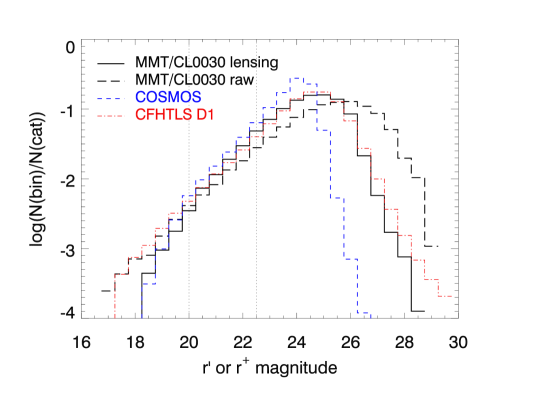
Figure 22: Source number counts in the CL0030+2618 and exemplary photometric redshift fields. Given are numbers of sources as fractions of the total number of objects in the $r^{\prime}$-band catalogue for the MMT Megacam CL0030+2618 raw (long-dashed curve) and lensing (before background selection; solid curve) catalogues as well as for the CFHTLS D1 field (dash-dotted curve). The dashed curve denotes the COSMOS $r^{+}$-band number counts. Vertical dotted lines indicate $m_{\mathrm{bright}}$ and $m_{\mathrm{faint}}$.

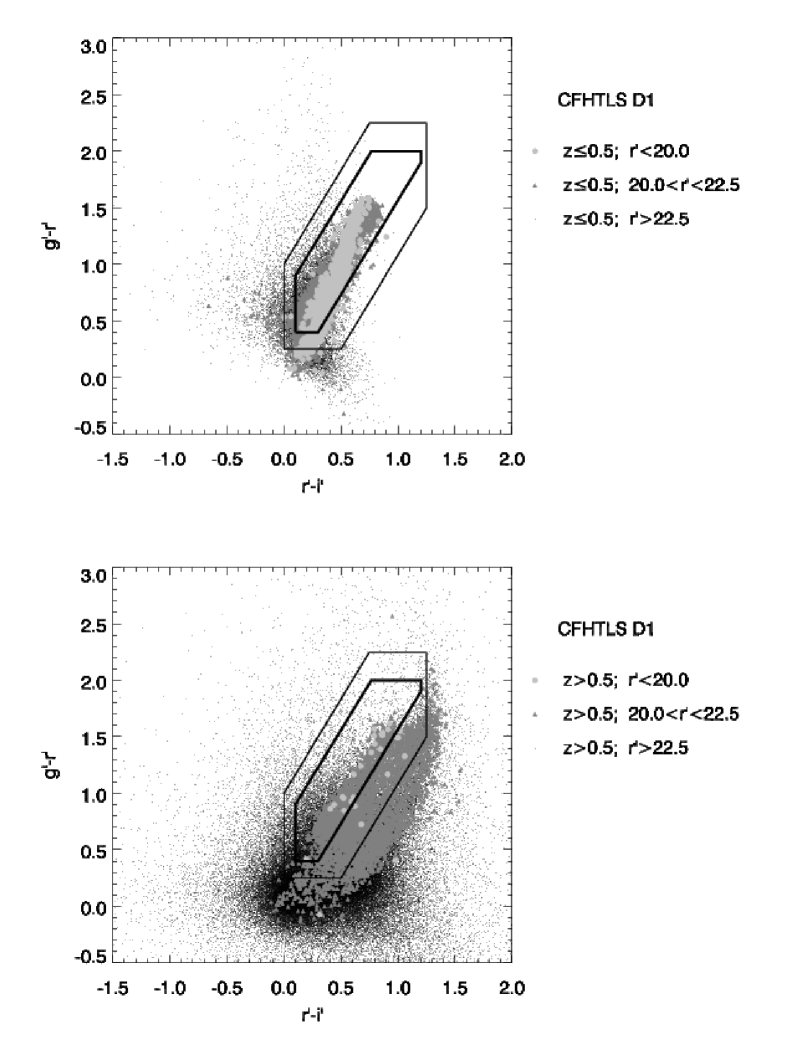
Figure 23: Colour-colour diagrammes of photo-$z$ galaxies in the CFHTLS D1 field. Shown are the $r^{\prime}\!-\!i^{\prime}$ against $g^{\prime}\!-\!r^{\prime}$ colours for foreground ($0.01\!<\!z\!\leq\!0.5$, upper panel) and background ($z\!>\!0.5$, lower panel) galaxies, divided into the three magnitude bins defined in Sect. B.2 and Fig. 20: $r^{\prime}\!<\!m_{\mathrm{bright}}\!=\!20.0$ (large symbols), $m_{\mathrm{bright}}\!<\!r^{\prime}\!<\!m_{\mathrm{faint}}$ (medium-sized symbols) and $r^{\prime}\!>\!m_{\mathrm{faint}}\!=\!22.5$ (small symbols). Also shown are the polygonals regions giving the locus of bright and intermediate galaxies in the CL0030+2618 field.

In order to check the significance of the optimal values empirically found for $m_{\mathrm{bright}}$ and $m_{\mathrm{faint}}$ – i.e., do they provide an effective distinction between galaxies at redshift $z\!\leq\!0.5$ and those at $z\!>\!0.5$? – and to estimate the geometric factor needed to convert gravitational shear into a mass estimate, we compare our data to two catalogues with known photometric redshift distributions, the CFHTLS Deep 1 field (Ilbert et al. 2006) and the COSMOS survey (Ilbert et al. 2009). In Fig. 22, we compare the source number counts as a function of magnitude of the MMT/Megacam catalogue of the CL0030+2618 field (before and after selection of high-quality shape objects, i.e. the unflagged SExctractor objects compared to the galaxy shape catalogue) to the CFHTLS D1 (MegaCam at CFHT, SDSS filter system) and COSMOS photo-z sources. For the latter, the Subaru $g^{+}r^{+}i^{+}$ magnitudes similar to the SDSS filters have been used. From the CFHTLS we use all unflagged sources classified as galaxies, detected in all five bands ($u^{*}g^{\prime}r^{\prime}i^{\prime}z^{\prime}$) and with a photo-$z$ derived from at least three bands whose $1\sigma$ error margin $\Delta z_{\mathrm{ph}}$ satisfies $\Delta z_{\mathrm{ph}}/(1+z_{\mathrm{ph}})\!<\!0.25$. Likewise, we use all unflagged sources classified as galaxies having an unflagged photo-$z$ estimate in the COSMOS catalogue that are detected in the Subaru $g^{+}r^{+}i^{+}$ and CFHT $i^{\prime}$ passbands.

Fig. 22 illustrates how the various cuts in the KSB pipeline remove faint galaxies from the catalogue, shifting the maximum $r^{\prime}_{\mathrm{mh}}$ of the histogramme from $r^{\prime}_{\mathrm{mh}}\!=\!26.0\pm 0.5$ to $r^{\prime}_{\mathrm{mh}}\!=\!25.0\pm 0.5$. We note that the CFHTLS D1 shows a very similar histogramme over most of the relevant magnitude range $20.5\!<\!r^{\prime}\!<\!27.0$, also peaking at $r^{\prime}_{\mathrm{mh}}\!=\!25.0\pm 0.5$. The other fields of the CFHTLS Deep Survey, D2 to D4, show a behaviour similar to D1 and are omitted from Fig. 22 for the sake of clarity. The COSMOS photo-z catalogue, on the other hand, is shallower, with $r^{+}_{\mathrm{mh}}\!=\!24.0\pm 0.5$, but showing a number count function similar to the one in the CL0030+2618 data at the bright end. Therefore, we use CFHTLS as a reference survey, estimating the relations between galaxy colours and photometric redshift in the CL0030+2618 data from the D1 field and using all fields to derive the redshift distribution.

B.3.1 Photometric Properties

First, we want to investigate the effect of the photometric cuts optimising the aperture mass detection on the redshift distribution of the CFHTLS D1 catalogue.

In Fig. 23, we compare the $r^{\prime}\!-\!i^{\prime}$ and $g^{\prime}\!-\!r^{\prime}$ colours of CFHTLS D1 galaxies with photometric redshift $0.01\!<\!z_{\mathrm{ph}}\!\leq\!0.5$ (upper panel) and $z_{\mathrm{ph}}\!>\!0.5$ (lower panel) to the polygonal regions found from Fig. 20 containing all bright ($r^{\prime}\!<\!20.0$) and most of the intermediate ($20.0\!<\!r^{\prime}\!<\!22.5$) galaxies in the CL0030+2618 field. The bright and intermediate nearby ($0.01\!<\!z_{\mathrm{ph}}\!\leq\!0.5$) galaxies indeed populate a similar region in the colour-colour diagramme like their Megacam counterparts, albeit being slightly shifted towards bluer $g^{\prime}\!-\!r^{\prime}$ colours. Thus, given its simplicity, our background selection is quite efficient for the $r^{\prime}\!<\!22.5$ foreground galaxies, removing $85$ % of them from the CFHTLS D1 catalogue. On the other hand, the number of bright ($r^{\prime}\!<\!20.0$) background ($z_{\mathrm{ph}}\!>\!0.5$) galaxies is negligible. Only $28$ % of the intermediary CFHTLS D1 background galaxies, redder in $r^{\prime}\!-\!i^{\prime}$ than the foreground sources but not in $g^{\prime}\!-\!r^{\prime}$, are removed by the selection criteria.

Concerning the faint ($r^{\prime}\!>\!22.5$) galaxy population, the first observe that, despite the similar source counts (Fig. 22), the colour distributions of faint sources in the CFHTLS D1 and CL0030+2618 fields differ qualitatively. Further investigations will be needed to relate this observation to a possible cause in the data reduction pipeline. This difference in the colour distributions affects the impact of the background selection: In contrast to the $6.0$ % sources removed as foregrounds from the CL0030+2618 catalogue, the size of the CFHTLS D1 catalogue is reduced by only $0.8$ %. (The rates differ little for the D2 to D4 fields.)

Second, we note the existence of a significant fraction of $z_{\mathrm{ph}}\!\leq\!0.5$ galaxies even to very faint magnitudes: we find $15$ % of the $r^{\prime}\!>\!22.5$ sources and $8$ % of the $r^{\prime}\!>\!25.0$ sources to be foregrounds to CL0030+2618, judging from their photo-$z$s. Consequently, our background selection cannot identify these sources, leading to a contamination of the lensing catalogue and a dilution of the lensing signal. Ilbert et al. (2006, their Fig. 16) and Ilbert et al. (2009, their Fig. 14) confirm the existence of this population of faint galaxies at low $z_{\mathrm{ph}}$. Although there certainly is a contribution by catastrophic outliers to which a $z_{\mathrm{ph}}\!\leq\!0.5$ has been assigned erroneously, the comparison with spectroscopic redshifts (Ilbert et al. 2006, their Fig. 12) indicates that most are indeed faint nearby galaxies.

Hence, applying the background selection to the whole catalogue, the rate of $z_{\mathrm{ph}}\!\leq\!0.5$ galaxies only drops from $18.2$ % to $17.6$ %. This indicates a similar level of residual contamination in the CL0030+2618 background catalogue (Sect. 6.2), given its redshift distribution follows the one in CFHTLS D1. We account for the shear dilution caused by foreground galaxies as a source of systematic uncertainty. To this end, we measure $18.0$ % galaxies at $z_{\mathrm{ph}}\!\leq\!0.5$ in the background-selected CFHTLS D1 catalogue, once the $2.2\!<\!g^{\prime}\!-\!i^{\prime}\!<\!3.0$ sources, already covered in the correction factor for cluster galaxies (Sect. 6.2) are excised. We consider this $18.0$ % uncertainty in the systematic error derived from shear calibration effects (Sect. 6.6).

B.3.2 Redshift Distribution

Figure 24: Photometric redshift distributions of the CFHTLS D1 to D4 fields after application of the photometric cuts defined in Sect. B.2 (histogrammes) and Van Waerbeke et al. (2001) best fits to these (solid lines). The function $D_{\mathrm{ds}}(z_{\mathrm{s}};z_{\mathrm{d}}\!=\!0.5)/D_{\mathrm{s}}(z_{\mathrm{s}})$ is denoted by dashed lines.

Table 10: Best fit parameters $z_{0}$, $A$ (fixed), and $B$ (fixed) of Eq. (22) to the CFHTLS D1 to D4 redshift distributions.

Field	$z_{0}$	$A$	$B$	$\operatorname{median}(z_{\mathrm{ph}})$	$\langle D_{\mathrm{ds}}/D_{\mathrm{s}}\rangle$
D1	$0.87$	$(1.15)$	$(1.5)$	$0.91$	$0.345$
D2	$0.76$	$(1.15)$	$(1.5)$	$0.79$	$0.297$
D3	$0.80$	$(1.15)$	$(1.5)$	$0.83$	$0.316$
D4	$0.90$	$(1.15)$	$(1.5)$	$0.95$	$0.358$

We use the redshift distribution in the CFHTLS Deep Fields to estimate $\langle D_{\mathrm{ds}}/D_{\mathrm{s}}\rangle$, the catalogue average of the ratio of angular diameter distances between deflector and source and source and observer. In the absence of (spectroscopic or photometric) redshifts of the individual galaxies, this essential quantity has to be determined from fields with a known redshift distribution.

In Fig. 24, we show the binned photometric redshift distributions we find for the CFHTLS D1 to D4 fields after having applied the same photometric cuts as to the CL0030+2618 data. The apparent spikes seen at certain redshifts in all the four fields are artifacts caused by the photo-$z$ determination. Because of those, we prefer calculating $\langle D_{\mathrm{ds}}/D_{\mathrm{s}}\rangle$ using a fit to the $z_{\mathrm{ph}}$-distribution. We choose a functional form introduced by Van Waerbeke et al. (2001):

$$p_{\mathrm{z}}(z_{\mathrm{ph}})\!=\!\frac{B}{z_{0}\Gamma\left(\frac{1+A}{B}\right)}\left(\frac{z_{\mathrm{ph}}}{z_{0}}\right)^{A}\exp\left(-\left(\frac{z_{\mathrm{ph}}}{z_{0}}\right)^{B}\right)$$ (22)

where $z_{0}$ is a typical redshift of the sources, and $A$ and $B$ shape parameters governing the low-redshift regime and the exponential drop-off at high redshifts. The prefactor including the Gamma function renders $p_{\mathrm{z}}(z_{\mathrm{ph}})$ a normalised probability distribution. We fit the binned redshift distributions in the range $0\!\leq\!z_{\mathrm{ph}}\!\leq\!4$, fixing $B\!=\!1.5$ for reasons of robustness to the default value suggested by Van Waerbeke et al. (2001). Next, $A\!=\!1.15$ is fixed too, to the value preferred for three of the four fields. The final results are summarised in Table LABEL:tab:zdist. Note that $D_{\mathrm{ds}}(z_{\mathrm{s}};z_{\mathrm{d}}\!=\!0.5)/D_{\mathrm{s}}(z_{\mathrm{s}})$ varies substantially over the range $0.8\!\lesssim\!\operatorname{median}(z_{\mathrm{ph}})\!\lesssim\!1.0$ spanned by the median redshifts of the fits to D1 to D4 (see Fig. 24). We now calculate the average distance ratio for each field by integrating this function with the redshift distribution over all redshifts larger than $z_{\mathrm{d}}\!=\!0.5$:

$$\Bigg{\langle}\frac{D_{\mathrm{ds}}}{D_{\mathrm{s}}}\Bigg{\rangle}\!=\!\int_{z_{\mathrm{d}}}^{\infty}{\!\!p_{\mathrm{z}}(z)\frac{D_{\mathrm{ds}}(z;z_{\mathrm{d}})}{D_{\mathrm{s}}(z)}\mathrm{d}z}$$ (23)

For the mass estimation of CL0030+2618, we use the average and standard deviation $\langle D_{\mathrm{ds}}/D_{\mathrm{s}}\rangle\!=\!0.33\pm 0.03$ of the distance ratios obtained for the four CFHTLS fields (see Table LABEL:tab:zdist) as fiducial value and uncertainty margin for the distance factor of our Megacam background sample. These values are consistent with the results for $\langle D_{\mathrm{ds}}/D_{\mathrm{s}}\rangle$ computed directly from the histogrammes in Fig. 24.