Resonant Perturbation Theory of Decoherence and Relaxation of Quantum Bits

Abstract

We describe our recent results on the resonant perturbation theory of decoherence and relaxation for quantum system with many qubits. The approach represents a rigorous analysis of the phenomenon of decoherence and relaxation for general $N$-level systems coupled to reservoirs of the bosonic fields. We derive a representation of the reduced dynamics valid for all times $t\geq 0$ and for small but fixed interaction strength. Our approach does not involve master equation approximations and applies to a wide variety of systems which are not explicitly solvable.

1 Introduction

Quantum computers (QCs) with large number of quantum bits (qubits) promise to solve important problems such as factorization of larger integer numbers, searching large unsorted databases, and simulations of physical processes exponentially faster than digital computers. Recently, many efforts were made for designing scalable (in the number of qubits) QC architectures based on solid-state implementations. One of the most promising designs of a solid-state QC is based on superconducting devices with Josephson junctions and solid-state quantum interference devices (SQUIDs) serving as qubits (effective spins), which operate in the quantum regime: $\hbar\omega>\!\!>k_{\rm B}T$, where $T$ is the temperature and $\omega$ is the qubit transition frequency. This condition is widely used in a superconducting quantum computation and quantum measurement, when $T\sim 10-20mK$ and $\hbar\omega\sim 100-150mK$ (in temperature units) [26, 15, 16, 27, 8, 25, 14, 4] (see also references therein). The main advantages of a QC with superconducting qubits are: (i) The two basic states of a qubit are represented by the states of a superconducting charge or current in the macroscopic (several $\mu m$ size) device. The relatively large scale of this device facilitates the manufacturing, and potential controlling and measuring of the states of qubits. (ii) The states of charge- and current-based qubits can be measured using rapidly developing technologies, such as a single electron transistor, effective resonant oscillators and micro-cavities with RF amplifiers, and quantum tunneling effects. (iii) The quantum logic operation can be implemented exclusively by switching locally on and off voltages on controlling micro-contacts and magnetic fluxes. (iv) The devices based on superconducting qubits can potentially achieve large quantum dephasing and relaxation times of milliseconds and more at low temperatures, allowing quantum coherent computation for long enough times. In spite of significant progress, current devices with superconducting qubits only have one or two qubits operating with low fidelity even for simplest operations.

One of the main problems which must be resolved in order to build a scalable QC is to develop novel approaches for suppression of unwanted effects such as decoherence and noise. This also requires to develop the rigorous mathematical tools for analyzing the dynamics of decoherence, entanglement and thermalization in order to control the quantum protocols with needed fidelity. These theoretical approaches must work for long enough times and be applicable to both solvable and not explicitly solvable (non-integrable) systems.

Here we present a review of our results [18, 19, 20] on the rigorous analysis of the phenomenon of decoherence and relaxation for general $N$-level systems coupled to reservoirs. The latter are described by the bosonic fields. We suggest a new approach which applies to a wide variety of systems which are not explicitly solvable. We analyze in detail the dynamics of an $N$-qubit quantum register collectively coupled to a thermal environment. Each spin experiences the same environment interaction, consisting of an energy conserving and an energy exchange part. We find the decay rates of the reduced density matrix elements in the energy basis. We show that the fastest decay rates of off-diagonal matrix elements induced by the energy conserving interaction is of order $N^{2}$, while the one induced by the energy exchange interaction is of the order $N$ only. Moreover, the diagonal matrix elements approach their limiting values at a rate independent of $N$. Our method is based on a dynamical quantum resonance theory valid for small, fixed values of the couplings, and uniformly in time for $t\geq 0$. We do not make Markov-, Born- or weak coupling (van Hove) approximations.

2 Presentation of results

We consider an $N$-level quantum system ${\rm S}$ interacting with a heat bath ${\rm R}$. The former is described by a Hilbert space ${\mathfrak{h}}_{s}={\mathbb{C}}^{N}$ and a Hamiltonian

$$H_{\rm S}={\rm diag}(E_{1},\ldots,E_{N}).$$ (2.1)

The environment ${\rm R}$ is modelled by a bosonic thermal reservoir with Hamiltonian

$$H_{\rm R}=\int_{{\mathbb{R}}^{3}}a^{*}(k)|k|a(k){\rm d}^{3}k,$$ (2.2)

acting on the reservoir Hilbert space ${\mathfrak{h}}_{\rm R}$, and where $a^{*}(k)$ and $a(k)$ are the usual bosonic creation and annihilation operators satisfying the canonical commutation relations $[a(k),a^{*}(l)]=\delta(k-l)$. It is understood that we consider ${\rm R}$ in the thermodynamic limit of infinite volume (${\mathbb{R}}^{3}$) and fixed temperature $T=1/\beta>0$ (in a phase without condensate). Given a form factor $f(k)$, a square integrable function of $k\in{\mathbb{R}}^{3}$ (momentum representation), the smoothed-out creation and annihilation operators are defined as $a^{*}(f)=\int_{{\mathbb{R}}^{3}}f(k)a^{*}(k){\rm d}^{3}k$ and $a(f)=\int_{{\mathbb{R}}^{3}}\overline{f(k)}a(k){\rm d}^{3}k$ respectively, and the hermitian field operator is

$$\phi(f)=\frac{1}{\sqrt{2}}\big{[}a^{*}(f)+a(f)\big{]}.$$ (2.3)

The total Hamiltonian, acting on ${\mathfrak{h}}_{\rm S}\otimes{\mathfrak{h}}_{\rm R}$, has the form

$$H=H_{\rm S}\otimes\mathchoice{\rm 1\mskip-4.0mul}{\rm 1\mskip-4.0mul}{\rm 1\mskip-4.5mul}{\rm 1\mskip-5.0mul}_{\rm R}+\mathchoice{\rm 1\mskip-4.0mul}{\rm 1\mskip-4.0mul}{\rm 1\mskip-4.5mul}{\rm 1\mskip-5.0mul}_{\rm S}\otimes H_{\rm R}+\lambda v,$$ (2.4)

where $\lambda$ is a coupling constant and $v$ is an interaction operator linear in field operators. For simplicity of exposition we consider here initial states where ${\rm S}$ and ${\rm R}$ are not entangled, and where ${\rm R}$ is in thermal equilibrium. The initial density matrix is thus

$$\rho_{0}={\overline{\rho}}_{0}\otimes\rho_{{\rm R},\beta},$$

where ${\overline{\rho}}_{0}$ is any state of ${\rm S}$ and $\rho_{{\rm R},\beta}$ is the equilibrium state of ${\rm R}$ at temperature $1/\beta$.

Let $A$ be an arbitrary observable of the system (an operator on the system Hilbert space ${\mathfrak{h}}_{\rm S}$) and set

$$\left\langle{A}\right\rangle_{t}:=\mbox{Tr}_{\rm S}({\overline{\rho}}_{t}A)=\mbox{Tr}_{{\rm S}+{\rm R}}(\rho_{t}(A\otimes\mathchoice{\rm 1\mskip-4.0mul}{\rm 1\mskip-4.0mul}{\rm 1\mskip-4.5mul}{\rm 1\mskip-5.0mul}_{\rm R})),$$ (2.5)

where $\rho_{t}$ is the density matrix of ${\rm S}+{\rm R}$ at time $t$ and

$${\overline{\rho}}_{t}={\rm Tr}_{{\rm R}}\rho_{t}$$

is the reduced density matrix of ${\rm S}$. In our approach, the dynamics of the reduced density matrix ${\overline{\rho}}_{t}$ is expressed in terms of the resonance structure of the system. Under the non-interacting dynamics ($\lambda=0$), the evolution of the reduced density matrix elements of ${\rm S}$, expressed in the energy basis $\{\varphi_{k}\}_{k=1}^{N}$ of $H_{\rm S}$, is given by

$$[{\overline{\rho}}_{t}]_{kl}=\left\langle{\varphi_{k}},{{\rm e}^{-{\rm i}tH_{\rm S}}{\overline{\rho}}_{0}{\rm e}^{{\rm i}tH_{\rm S}}\varphi_{l}}\right\rangle={\rm e}^{{\rm i}te_{lk}}[{\overline{\rho}}_{0}]_{kl},$$ (2.6)

where $e_{lk}=E_{l}-E_{k}$. As the interaction with the reservoir is turned on, the dynamics (2.6) undergoes two qualitative changes.

• The “Bohr frequencies”

  $$e\in\{E-E^{\prime}\ :E,E^{\prime}\in{\rm spec}(H_{\rm S})\}$$ (2.7)

  in the exponent of (2.6) become complex, $e\mapsto\varepsilon_{e}$. It can be shown generally that the resonance energies $\varepsilon_{e}$ have non-negative imaginary parts, ${\rm Im}\varepsilon_{e}\geq 0$. If ${\rm Im}\varepsilon_{e}>0$ then the corresponding dynamical process is irreversible.

• The matrix elements do not evolve independently any more. Indeed, the effective energy of ${\rm S}$ is changed due to the interaction with the reservoirs, leading to a dynamics that does not leave eigenstates of $H_{\rm S}$ invariant. (However, to lowest order in the interaction, the eigenspaces of $H_{\rm S}$ are left invariant and therefore matrix elements with $(m,n)$ belonging to a fixed energy difference $E_{m}-E_{n}$ will evolve in a coupled manner.)

Our goal is to derive these two effects from the microscopic (hamiltonian) model and to quantify them. Our analysis yields the thermalization and decoherence times of quantum registers.

2.1 Evolution of reduced dynamics of an $N$-level system

Let $A\in{\cal B}({\mathfrak{h}}_{\rm S})$ be an observable of the system ${\rm S}$. We show in [18, 19] that the ergodic averages

$$\left\langle{\left\langle{A}\right\rangle}\right\rangle_{\infty}:=\lim_{T\rightarrow\infty}\frac{1}{T}\int_{0}^{T}\left\langle{A}\right\rangle_{t}{\rm d}t$$ (2.8)

exist, i.e., that $\left\langle{A}\right\rangle_{t}$ converges in the ergodic sense as $t\rightarrow\infty$. Furthermore, we show that for any $t\geq 0$ and for any $0<\omega^{\prime}<2\pi/\beta$,

$$\left\langle{A}\right\rangle_{t}-\left\langle{\left\langle{A}\right\rangle}\right\rangle_{\infty}=\sum_{\varepsilon\neq 0}{\rm e}^{{\rm i}t\varepsilon}R_{\varepsilon}(A)+O\left(\lambda^{2}{\rm e}^{-[\omega^{\prime}-O(\lambda)]t}\right),$$ (2.9)

where the complex numbers $\varepsilon$ are the eigenvalues of a certain explicitly given operator $K(\omega^{\prime})$, lying in the strip $\{z\in{\mathbb{C}}\ |\ 0\leq{\mathrm{I}m}z<\omega^{\prime}/2\}$. They have the expansions

$$\varepsilon\equiv\varepsilon_{e}^{(s)}=e+\lambda^{2}\delta_{e}^{(s)}+O(\lambda^{4}),$$ (2.10)

where $e\in{\mathrm{s}pec}(H_{\rm S}\otimes\mathchoice{\rm 1\mskip-4.0mul}{\rm 1\mskip-4.0mul}{\rm 1\mskip-4.5mul}{\rm 1\mskip-5.0mul}_{\rm S}-\mathchoice{\rm 1\mskip-4.0mul}{\rm 1\mskip-4.0mul}{\rm 1\mskip-4.5mul}{\rm 1\mskip-5.0mul}_{\rm S}\otimes H_{\rm S})={\mathrm{s}pec}(H_{\rm S})-{\mathrm{s}pec}(H_{\rm S})$ and the $\delta_{e}^{(s)}$ are the eigenvalues of a matrix $\Lambda_{e}$, called a level-shift operator, acting on the eigenspace of $H_{\rm S}\otimes\mathchoice{\rm 1\mskip-4.0mul}{\rm 1\mskip-4.0mul}{\rm 1\mskip-4.5mul}{\rm 1\mskip-5.0mul}_{\rm S}-\mathchoice{\rm 1\mskip-4.0mul}{\rm 1\mskip-4.0mul}{\rm 1\mskip-4.5mul}{\rm 1\mskip-5.0mul}_{\rm S}\otimes H_{\rm S}$ corresponding to the eigenvalue $e$ (which is a subspace of ${\mathfrak{h}}_{\rm S}\otimes{\mathfrak{h}}_{\rm S}$). The $R_{\varepsilon}(A)$ in (2.9) are linear functionals of $A$ and are given in terms of the initial state, $\rho_{0}$, and certain operators depending on the Hamiltonian $H$. They have the expansion

$$R_{\varepsilon}(A)=\sum_{(m,n)\in I_{e}}\varkappa_{m,n}A_{m,n}+O(\lambda^{2}),$$ (2.11)

where $I_{e}$ is the collection of all pairs of indices such that $e=E_{m}-E_{n}$, the $E_{k}$ being the eigenvalues of $H_{\rm S}$. Here, $A_{m,n}$ is the $(m,n)$-matrix element of the observable $A$ in the energy basis of $H_{\rm S}$, and the $\varkappa_{m,n}$ are coefficients depending on the initial state of the system (and on $e$, but not on $A$ nor on $\lambda$).

Discussion.  – In the absence of interaction ($\lambda=0$) we have $\varepsilon=e\in{\mathbb{R}}$, see (2.10). Depending on the interaction each resonance energy $\varepsilon$ may migrate into the upper complex plane, or it may stay on the real axis, as $\lambda\neq 0$.

– The averages $\left\langle{A}\right\rangle_{t}$ approach their ergodic means $\left\langle{\left\langle{A}\right\rangle}\right\rangle_{\infty}$ if and only if ${\rm Im}\varepsilon>0$ for all $\varepsilon\neq 0$. In this case the convergence takes place on the time scale $[{\mathrm{I}m}\varepsilon]^{-1}$. Otherwise $\left\langle{A}\right\rangle_{t}$ oscillates. A sufficient condition for decay is that ${\rm Im}\delta_{e}^{(s)}>0$ (and $\lambda$ small, see (2.10)).

– The error term in (2.9) is small in $\lambda$, uniformly in $t\geq 0$, and it decays in time quicker than any of the main terms in the sum on the r.h.s.: indeed, ${\rm Im}\varepsilon=O(\lambda^{2})$ while $\omega^{\prime}-O(\lambda)>\omega^{\prime}/2$ independent of small values of $\lambda$. However, this means that we are in the regime $\lambda^{2}<\!\!<\omega^{\prime}<2\pi/\beta$ (see before (2.9)), which implies that $\lambda^{2}$ must be much smaller than the temperature $T=1/\beta$. Using a more refined analysis one can get rid of this condition, see also remarks on p.376 of [19].

– Relation (2.11) shows that to lowest order in the perturbation the group of (energy basis) matrix elements of any observable $A$ corresponding to a fixed energy difference $E_{m}-E_{n}$ evolve jointly, while those of different such groups evolve independently.

It is well known that there are two kinds of processes which drive decay (or irreversibility) of ${\rm S}$: energy-exchange processes characterized by $[v,H_{\rm S}]\neq 0$ and energy preserving ones where $[v,H_{\rm S}]=0$. The former are induced by interactions having nonvanishing probabilities for processes of absorption and emission of field quanta with energies corresponding to the Bohr frequencies of ${\rm S}$ and thus typically inducing thermalization of ${\rm S}$. Energy preserving interactions suppress such processes, allowing only for a phase change of the system during the evolution (“phase damping”, [23, 3, 7, 10, 13, 22, 24]).

To our knowledge, energy-exchange systems have so far been treated using Born and Markov master equation approximations (Lindblad form of dynamics) or they have been studied numerically, while for energy conserving systems one often can find an exact solution. The present representation (2.9) gives a detailed picture of the dynamics of averages of observables for interactions with and without energy exchange. The resonance energies $\varepsilon$ and the functionals $R_{\varepsilon}$ can be calculated for concrete models, as illustrated in the next section. We mention that the resonance dynamics representation can be used to study the dynamics of entanglement of qubits coupled to local and collective reservoirs. Work on this is in progress.

Contrast with weak coupling approximation.  Our representation (2.9) of the true dynamics of ${\rm S}$ relies only on the smallness of the coupling parameter $\lambda$, and no approximation is made. In the absence of an exact solution, it is common to make a weak coupling Lindblad master equation approximation of the dynamics, in which the reduced density matrix evolves according to ${\overline{\rho}}_{t}={\rm e}^{t{\cal L}}{\overline{\rho}}_{0}$, where $\cal L$ is the Lindblad generator, [2, 5, 6]. This approximation can lead to results that differ qualitatively from the true behaviour. For instance, the Lindblad master equation predicts that the system ${\rm S}$ approaches its Gibbs state at the temperature of the reservoir in the limit of large times. However, it is clear that in reality, the coupled system ${\rm S}+{\rm R}$ will approach equilibrium, and hence the asymptotic state of ${\rm S}$ alone, being the reduction of the coupled equilibrium state, is the Gibbs state of ${\rm S}$ only to first approximation in the coupling (see also illustration below, and references [18, 19]). In particular, the system’s asymptotic density matrix is not diagonal in the original energy basis, but it has off-diagonal matrix elements of $O(\lambda^{2})$. Features of this kind cannot be captured by the Lindblad approximation, but are captured in our approach.

It has been shown (see e.g. [9, 5, 6, 12]) that the weak coupling limit dynamics generated by the Lindblad operator is obtained in the regime $\lambda\rightarrow 0$, $t\rightarrow\infty$, with $t/\lambda^{2}$ fixed. One of the strengths of our approach is that we do not impose any relation between $\lambda$ and $t$, and our results are valid for all times $t\geq 0$, provided $\lambda$ is small. It has been observed [9, 12] that for certain systems of the type ${\rm S}+{\rm R}$, the second order contribution of the exponents $\varepsilon_{e}^{(s)}$ in (2.10) correspond to eigenvalues of the Lindblad generator. Our resonance method gives the true exponents, i.e., we do not lose the contributions of any order in the interaction. If the energy spectrum of $H_{\rm S}$ is degenerate, it happens that the second order contributions to ${\rm Im}\varepsilon_{e}^{(s)}$ vanish. This corresponds to a Lindblad generator having several real eigenvalues. In this situation the correct dynamics (approach to a final state) can be captured only by taking into account higher order contributions to the exponents $\varepsilon_{e}^{(s)}$, see [17]. To our knowledge, so far this can only be done with the method presented in this paper, and is beyond the reach of the weak coupling method.

Illustration: single qubit.  Consider ${\rm S}$ to be a single spin $1/2$ with energy gap $\Delta=E_{2}-E_{1}>0$. ${\rm S}$ is coupled to the heat bath ${\rm R}$ via the operator

$$v=\left[\begin{array}[]{cc}a&c\\ \overline{c}&b\end{array}\right]\otimes\phi(g),$$ (2.12)

where $\phi(g)$ is the Bose field operator (2.3), smeared out with a coupling function (form factor) $g(k)$, $k\in{\mathbb{R}}^{3}$, and the $2\times 2$ coupling matrix (representing the coupling operator in the energy eigenbasis) is hermitian. The operator (2.12) - or a sum of such terms, for which our technique works equally well - is the most general coupling which is linear in field operators. We refer to [19] for a discussion of the link between (2.12) and the spin-boson model. We take ${\rm S}$ initially in a coherent superposition in the energy basis,

$${\overline{\rho}}_{0}=\textstyle\frac{1}{2}\left[\begin{array}[]{cc}1&1\\ 1&1\end{array}\right].$$ (2.13)

In [19] we derive from representation (2.9) the following expressions for the dynamics of matrix elements, for all $t\geq 0$:

$$[{\overline{\rho}}_{t}]_{m,m} = \frac{{\rm e}^{-\beta E_{m}}}{Z_{{\rm S},\beta}}+\frac{(-1)^{m}}{2}\tanh\left(\frac{\beta\Delta}{2}\right){\rm e}^{{\rm i}t\varepsilon_{0}(\lambda)}+R_{m,m}(\lambda,t),\ \ \ m=1,2,\ \$$ (2.14)

$${}[{\overline{\rho}}_{t}]_{1,2} = {\textstyle\frac{1}{2}}{\rm e}^{{\rm i}t\varepsilon_{-\Delta}(\lambda)}+R_{1,2}(\lambda,t),$$ (2.15)

where the resonance energies $\varepsilon$ are given by

$$\varepsilon_{0}(\lambda) = {\rm i}\lambda^{2}\pi^{2}|c|^{2}\xi(\Delta)+O(\lambda^{4})$$

$$\varepsilon_{\Delta}(\lambda) = \Delta+\lambda^{2}R+{\textstyle\frac{{\rm i}}{2}}\lambda^{2}\pi^{2}\left[|c|^{2}\xi(\Delta)+(b-a)^{2}\xi(0)\right]+O(\lambda^{4})$$ (2.16)

$$\varepsilon_{-\Delta}(\lambda) = -\overline{\varepsilon_{\Delta}(\lambda)}$$

with

$$\xi(\eta)=\lim_{\epsilon\downarrow 0}\frac{1}{\pi}\int_{{\mathbb{R}}^{3}}{\rm d}^{3}k\coth\!\left(\frac{\beta|k|}{2}\right)|g(k)|^{2}\frac{\epsilon}{(|k|-\eta)^{2}+\epsilon^{2}},$$ (2.17)

and

$$R={\textstyle\frac{1}{2}}(b^{2}-a^{2})\left\langle{g},{\omega^{-1}g}\right\rangle$$

$$+{\textstyle\frac{1}{2}}|c|^{2}{\rm P.V.}\int_{{\mathbb{R}}\times S^{2}}u^{2}|g(|u|,\sigma)|^{2}\coth\!\left(\frac{\beta|u|}{2}\right)\frac{1}{u-\Delta}.$$

The remainder terms in (2.14), (2.15) satisfy $|R_{m,n}(\lambda,t)|\leq C\lambda^{2}$, uniformly in $t\geq 0$, and they can be decomposed into a sum of a constant and a decaying part,

$$R_{m,n}(\lambda,t)=\left\langle{\left\langle{p_{n,m}}\right\rangle}\right\rangle_{\infty}-\delta_{m,n}\frac{{\rm e}^{-\beta E_{m}}}{Z_{{\rm S},\beta}}+R^{\prime}_{m,n}(\lambda,t),$$

where $|R^{\prime}_{m,n}(\lambda,t)|=O(\lambda^{2}{\rm e}^{-\gamma t})$, with $\gamma=\min\{{\rm Im}\varepsilon_{0},{\rm Im}\varepsilon_{\pm\Delta}\}$. These relations show that

– To second order in $\lambda$, convergence of the populations to the equilibrium values (Gibbs law), and decoherence occur exponentially fast, with rates $\tau_{T}=[{\mathrm{I}m}\varepsilon_{0}(\lambda)]^{-1}$ and $\tau_{D}=[{\mathrm{I}m}\varepsilon_{\Delta}(\lambda)]^{-1}$, respectively. (If either of these imaginary parts vanishes then the corresponding process does not take place, of course.) In particular, coherence of the initial state stays preserved on time scales of the order $\lambda^{-2}[|c|^{2}\xi(\Delta)+(b-a)^{2}\xi(0)]^{-1}$, c.f. (2.16).

– The final density matrix of the spin is not the Gibbs state of the qubit, and it is not diagonal in the energy basis. The deviation of the final state from the Gibbs state is given by $\lim_{t\rightarrow\infty}R_{m,n}(\lambda,t)=O(\lambda^{2})$. This is clear heuristically too, since typically the entire system ${\rm S}+{\rm R}$ approaches its joint equilibrium in which ${\rm S}$ and ${\rm R}$ are entangled. The reduction of this state to ${\rm S}$ is the Gibbs state of ${\rm S}$ modulo $O(\lambda^{2})$ terms representing a shift in the effective energy of ${\rm S}$ due to the interaction with the bath. In this sense, coherence in the energy basis of ${\rm S}$ is created by thermalization. We have quantified this in [19], Theorem 3.3.

– In a markovian master equation approach the above phenomenon (i.e., variations of $O(\lambda^{2})$ in the time-asymptotic limit) cannot be detected. Indeed in that approach one would conclude that ${\rm S}$ approaches its Gibbs state as $t\rightarrow\infty$.

2.2 Collective decoherence of a qubit register

In the sequel we analyze in more detail the evolution of a qubit register of size $N$. The Hamiltonian is

$$H_{\rm S}=\sum_{i,j=1}^{N}J_{ij}S^{z}_{i}S^{z}_{j}+\sum_{j=1}^{N}B_{j}S_{j}^{z},$$ (2.18)

where the $J_{ij}$ are pair interaction constants and $B_{j}$ is the value of a magnetic field at the location of spin $j$. The Pauli spin operator is

$$S^{z}=\left[\begin{array}[]{cc}1&0\\ 0&-1\end{array}\right]$$ (2.19)

and $S_{j}^{z}$ is the matrix $S^{z}$ acting on the $j$-th spin only.

We consider a collective coupling between the register ${\rm S}$ and the reservoir ${\rm R}$: the distance between the $N$ qubits is much smaller than the correlation length of the reservoir and as a consequence, each qubit feels the same interaction with the reservoir. The corresponding interaction operator is (compare with (2.4))

$$\lambda_{1}v_{1}+\lambda_{2}v_{2}=\lambda_{1}\sum_{j=1}^{N}S_{j}^{z}\otimes\phi(g_{1})+\lambda_{2}\sum_{j=1}^{N}S_{j}^{x}\otimes\phi(g_{2}).$$ (2.20)

Here $g_{1}$ and $g_{2}$ are form factors and the coupling constants $\lambda_{1}$ and $\lambda_{2}$ measure the strengths of the energy conserving (position-position) coupling, and the energy exchange (spin flip) coupling, respectively. Spin-flips are implemented by the $S_{j}^{x}$ in (2.20), representing the Pauli matrix

$$S^{x}=\ \left[\begin{array}[]{cc}0&1\\ 1&0\end{array}\right]$$ (2.21)

acting on the $j$-th spin. The total Hamiltonian takes the form (2.4) with $\lambda v$ replaced by (2.20). It is convenient to represent ${\overline{\rho}}_{t}$ as a matrix in the energy basis, consisting of eigenvectors $\varphi_{\underline{\,\sigma\!}\,}$ of $H_{\rm S}$. These are vectors in ${\mathfrak{h}}_{\rm S}={\mathbb{C}}^{2}\otimes\cdots\otimes{\mathbb{C}}^{2}={\mathbb{C}}^{2^{N}}$ indexed by spin configurations

$${\underline{\,\sigma\!}\,}=\{\sigma_{1},\ldots,\sigma_{N}\}\in\{+1,-1\}^{N},\qquad\varphi_{\underline{\,\sigma\!}\,}=\varphi_{\sigma_{1}}\otimes\cdots\otimes\varphi_{\sigma_{N}},$$ (2.22)

where

$$\varphi_{+}=\left[\begin{array}[]{c}1\\ 0\end{array}\right],\quad\varphi_{-}=\left[\begin{array}[]{c}0\\ 1\end{array}\right],$$ (2.23)

so that

$$H_{\rm S}\varphi_{\underline{\,\sigma\!}\,}=E({\underline{\,\sigma\!}\,})\varphi_{\underline{\,\sigma\!}\,}\mbox{\qquad with \qquad}E({\underline{\,\sigma\!}\,})=\sum_{i,j=1}^{N}J_{ij}\sigma_{i}\sigma_{j}+\sum_{j=1}^{N}B_{j}\sigma_{j}.$$ (2.24)

We denote the reduced density matrix elements as

$$[{\overline{\rho}}_{t}]_{{\underline{\,\sigma\!}\,},{\underline{\,\tau\!}\,}}=\left\langle{\varphi_{\underline{\,\sigma\!}\,}},{{\overline{\rho}}_{t}\varphi_{\underline{\,\tau\!}\,}}\right\rangle.$$ (2.25)

The Bohr frequencies (2.7) are now

$$e({\underline{\,\sigma\!}\,},{\underline{\,\tau\!}\,})=E({\underline{\,\sigma\!}\,})-E({\underline{\,\tau\!}\,})=\sum_{i,j=1}^{N}J_{ij}(\sigma_{i}\sigma_{j}-\tau_{i}\tau_{j})+\sum_{j=1}^{N}B_{j}(\sigma_{j}-\tau_{j})$$ (2.26)

and they become complex resonance energies $\varepsilon_{e}=\varepsilon_{e}(\lambda_{1},\lambda_{2})\in{\mathbb{C}}$ under perturbation.

Assumption of non-overlapping resonances.  The Bohr frequencies (2.26) represent “unperturbed” energy levels and we follow their motion under perturbation ($\lambda_{1},\lambda_{2}$). In this work, we consider the regime of non-overlapping resonances, meaning that the interaction is small relative to the spacing of the Bohr frequencies.

We show in [19], Theorem 2.1, that for all $t\geq 0$,

$$[{\overline{\rho}}_{t}]_{{\underline{\,\sigma\!}\,},{\underline{\,\tau\!}\,}}-\langle\!\langle[{\overline{\rho}}_{\infty}]_{{\underline{\,\sigma\!}\,},{\underline{\,\tau\!}\,}}\rangle\!\rangle = \sum_{\{e:\ \varepsilon_{e}\neq 0\}}{\rm e}^{{\rm i}t\varepsilon_{e}}\Big{[}\sum_{{\underline{\,\sigma\!}\,}^{\prime},{\underline{\,\tau\!}\,}^{\prime}}w^{\varepsilon_{e}}_{{\underline{\,\sigma\!}\,},{\underline{\,\tau\!}\,};{\underline{\,\sigma\!}\,}^{\prime},{\underline{\,\tau\!}\,}^{\prime}}\ [{\overline{\rho}}_{0}]_{{\underline{\,\sigma\!}\,}^{\prime},{\underline{\,\tau\!}\,}^{\prime}}+O(\lambda_{1}^{2}+\lambda_{2}^{2})\Big{]}$$ (2.27)

$$+O\big{(}(\lambda_{1}^{2}+\lambda_{2}^{2}){\rm e}^{-[\omega^{\prime}+O(\lambda)]t}\big{)}.$$

This result is obtained by specializing (2.9) to the specific system at hand and considering observables $A=|\varphi_{\underline{\,\tau\!}\,}\rangle\langle\varphi_{\underline{\,\sigma\!}\,}|$. In (2.27), we have in accordance with (2.8) $\langle\!\langle[{\overline{\rho}}_{\infty}]_{{\underline{\,\sigma\!}\,},{\underline{\,\tau\!}\,}}\rangle\!\rangle=\lim_{T\rightarrow\infty}\frac{1}{T}\int_{0}^{T}[{\overline{\rho}}_{t}]_{{\underline{\,\sigma\!}\,},{\underline{\,\tau\!}\,}}\ {\rm d}t$. The coefficients $w$ are overlaps of resonance eigenstates which vanish unless $e=-e({\underline{\,\sigma\!}\,},{\underline{\,\tau\!}\,})=-e({\underline{\,\sigma\!}\,}^{\prime},{\underline{\,\tau\!}\,}^{\prime})$ (see point 2. after (2.7)). They represent the dominant contribution to the functionals $R_{\varepsilon}$ in (2.9), see also (2.11). The $\varepsilon_{e}$ have the expansion

$$\varepsilon_{e}\equiv\varepsilon^{(s)}_{e}=e+\delta_{e}^{(s)}+O(\lambda_{1}^{4}+\lambda_{2}^{4}),$$ (2.28)

where the label $s=1,\ldots,\nu(e)$ indexes the splitting of the eigenavlue $e$ into $\nu(e)$ distinct resonance energies. The lowest order corrections $\delta_{e}^{(s)}$ satisfy

$$\delta_{e}^{(s)}=O(\lambda_{1}^{2}+\lambda_{2}^{2}).$$ (2.29)

They are the (complex) eigenvalues of an operator $\Lambda_{e}$, called the level shift operator associated to $e$. This operator acts on the eigenspace of $L_{\rm S}$ associated to the eigenvalue $e$ (a subspace of the qubit register Hilbert space; see [19, 20] for the formal definition of $\Lambda_{e}$). It governs the lowest order shift of eigenvalues under perturbation. One can see by direct calculation that ${\rm Im}\delta_{e}^{(s)}\geq 0$.

Discussion.  – To lowest order in the perturbation, the group of reduced density matrix elements $[{\overline{\rho}}_{t}]_{{\underline{\,\sigma\!}\,},{\underline{\,\tau\!}\,}}$ associated to a fixed $e=e({\underline{\,\sigma\!}\,},{\underline{\,\tau\!}\,})$ evolve in a coupled way, while groups of matrix elements associated to different $e$ evolve independently.

– The density matrix elements of a given group mix and evolve in time according to the weight functions $w$ and the exponentials ${\rm e}^{{\rm i}t\varepsilon_{e}^{(s)}}$. In the absence of interaction ($\lambda_{1}=\lambda_{2}=0$) all the $\varepsilon_{e}^{(s)}=e$ are real. As the interaction is switched on, the $\varepsilon_{e}^{(s)}$ typically migrate into the upper complex plane, but they may stay on the real line (due to some symmetry or due to an ‘inefficient coupling’).

– The matrix elements $[{\overline{\rho}}_{t}]_{{\underline{\,\sigma\!}\,},{\underline{\,\tau\!}\,}}$ of a group $e$ approach their ergodic means if and only if all the nonzero $\varepsilon_{e}^{(s)}$ have strictly positive imaginary part. In this case the convergence takes place on a time scale of the order $1/\gamma_{e}$, where

$$\gamma_{e}=\min\left\{{\rm Im}\varepsilon_{e}^{(s)}:\ s=1,\ldots,\nu(e){\ \rm s.t.\ }\varepsilon_{e}^{(s)}\neq 0\right\}$$ (2.30)

is the decay rate of the group associated to $e$. If an $\varepsilon_{e}^{(s)}$ stays real then the matrix elements of the corresponding group oscillate in time. A sufficient condition for decay of the group associated to $e$ is $\gamma_{e}>0$, i.e. ${\rm Im}\delta_{e}^{(s)}>0$ for all $s$, and $\lambda_{1}$, $\lambda_{2}$ small.

Decoherence rates.  We illustrate our results on decoherence rates for a qubit register with $J_{ij}=0$ (the general case is treated in [20]). We consider generic magnetic fields defined as follows. For $n_{j}\in\{0,\pm 1,\pm 2\}$, $j=1,\ldots,N$, we have

$$\sum_{j=1}^{N}B_{j}n_{j}=0\qquad\Longleftrightarrow\qquad n_{j}=0\ \forall j.$$ (2.31)

Condition (2.31) is satisfied generically in the sense that only for very special choices of $B_{j}$ does it not hold (one such special choice is $B_{j}={\mbox{c}onstant}$). For instance, if the $B_{j}$ are chosen to be independent, and uniformly random from an interval $[B_{\rm min},B_{\rm max}]$, then (2.31) is satisfied with probability one. We show in [20], Theorem 2.3, that the decoherence rates (2.30) are given by

$$\gamma_{e}=\left\{\begin{array}[]{ll}\lambda_{1}^{2}y_{1}(e)+\lambda_{2}^{2}y_{2}(e)+y_{12}(e),&e\neq 0\\ \lambda_{2}^{2}y_{0},&e=0\end{array}\right\}+O(\lambda_{1}^{4}+\lambda_{2}^{4}).$$ (2.32)

Here, $y_{1}$ is a contributions coming from the energy conserving interaction, $y_{0}$ and $y_{2}$ are due to the spin flip interaction. The term $y_{12}$ is due to both interactions and is of $O(\lambda^{2}_{1}+\lambda^{2}_{2})$. We give explicit expressions for $y_{0}$, $y_{1}$, $y_{2}$ and $y_{12}$ in [20], Section 2. For the present purpose, we limit ourselves to discussing the properties of the latter quantities.

• Properties of $y_{1}(e)$: $y_{1}(e)$ vanishes if either $e$ is such that $e_{0}:=\sum_{j=1}^{n}(\sigma_{j}-\tau_{j})=0$, or the infra-red behaviour of the coupling function $g_{1}$ is too regular (in three dimensions $g_{1}\propto|k|^{p}$ with $p>-1/2$). Otherwise $y_{1}(e)>0$. Moreover, $y_{1}(e)$ is proportional to the temperature $T$.

• Properties of $y_{2}(e)$: $y_{2}(e)>0$ if $g_{2}(2B_{j},\Sigma)\neq 0$ for all $B_{j}$ (form factor $g_{2}(k)=g_{2}(|k|,\Sigma)$ in spherical coordinates). For low temperatures $T$, $y_{2}(e)\propto T$, for high temperatures $y_{2}(e)$ approaches a constant.

• Properties of $y_{12}(e)$: If either of $\lambda_{1}$, $\lambda_{2}$ or $e_{0}$ vanish, or if $g_{1}$ is infra-red regular as mentioned above, then $y_{12}(e)=0$. Otherwise $y_{12}(e)>0$, in which case $y_{12}(e)$ approaches constant values for both $T\rightarrow 0,\infty$.

• Full decoherence: If $\gamma_{e}>0$ for all $e\neq 0$ then all off-diagonal matrix elements approach their limiting values exponentially fast. In this case we say that full decoherence occurs. It follows from the above points that we have full decoherence if $\lambda_{2}\neq 0$ and $g_{2}(2B_{j},\Sigma)\neq 0$ for all $j$, and provided $\lambda_{1},\lambda_{2}$ are small enough (so that the remainder term in (2.32) is small). Note that if $\lambda_{2}=0$ then matrix elements associated to energy differences $e$ such that $e_{0}=0$ will not decay on the time scale given by the second order in the perturbation ($\lambda_{1}^{2}$).
  We point out that generically, ${\rm S}+{\rm R}$ will reach a joint equilibrium as $t\rightarrow\infty$, which means that the final reduced density matrix of ${\rm S}$ is its Gibbs state modulo a peturbation of the order of the interaction between ${\rm S}$ and ${\rm R}$, see [18, 19]. Hence generically, the density matrix of ${\rm S}$ does not become diagonal in the energy basis as $t\rightarrow\infty$.

• Properties of $y_{0}$: $y_{0}$ depends on the energy exchange interaction only. This reflects the fact that for a purely energy conserving interaction, the populations are conserved [18, 19, 23]. If $g_{2}(2B_{j},\Sigma)\neq 0$ for all $j$, then $y_{0}>0$ (this is sometimes called the “Fermi Golden Rule Condition”). For small temperatures $T$, $y_{0}\propto T$, while $y_{0}$ approaches a finite limit as $T\rightarrow\infty$.

In terms of complexity analysis, it is important to discuss the dependence of $\gamma_{e}$ on the register size $N$.

• We show in [20] that $y_{0}$ is independent of $N$. This means that the thermalization time, or relaxation time of the diagonal matrix elements (corresponding to $e=0$), is $O(1)$ in $N$.

• To determine the order of magnitude of the decay rates of the off-diagonal density matrix elements (corresponding to $e\neq 0$) relative to the register size $N$, we assume the magnetic field to have a certain distribution denoted by $\left\langle{\ }\right\rangle$. We show in [20] that

  $$\left\langle{y_{1}}\right\rangle=y_{1}\propto e_{0}^{2},\quad\left\langle{y_{2}}\right\rangle=C_{B}{\mathfrak{D}}({\underline{\,\sigma\!}\,}-{\underline{\,\tau\!}\,}),\quad\mbox{and}\quad\left\langle{y_{12}}\right\rangle=c_{B}(\lambda_{1},\lambda_{2})N_{0}(e),$$ (2.33)

  where $C_{B}$ and $c_{B}=c_{B}(\lambda_{1},\lambda_{2})$ are positive constants (independent of $N$), with $c_{B}(\lambda_{1},\lambda_{2})=O(\lambda_{1}^{2}+\lambda_{2}^{2})$. Here, $N_{0}(e)$ is the number of indices $j$ such that $\sigma_{j}=\tau_{j}$ for each $({\underline{\,\sigma\!}\,},{\underline{\,\tau\!}\,})$ s.t. $e({\underline{\,\sigma\!}\,},{\underline{\,\tau\!}\,})=e$, and

  $${\mathfrak{D}}({\underline{\,\sigma\!}\,}-{\underline{\,\tau\!}\,}):=\sum_{j=1}^{N}|\sigma_{j}-\tau_{j}|$$ (2.34)

  is the Hamming distance between the spin configurations ${\underline{\,\sigma\!}\,}$ and ${\underline{\,\tau\!}\,}$ (which depends on $e$ only).

• Consider $e\neq 0$. It follows from (2.32)-(2.34) that for purely energy conserving interactions ($\lambda_{2}=0$), $\gamma_{e}\propto\lambda_{1}^{2}e_{0}^{2}=\lambda_{1}^{2}[\sum_{j=1}^{N}(\sigma_{j}-\tau_{j})]^{2}$, which can be as large as $O(\lambda_{1}^{2}N^{2})$. On the other hand, for purely energy exchanging interactions ($\lambda_{1}=0$), we have $\gamma_{e}\propto\lambda_{2}^{2}{\mathfrak{D}}({\underline{\,\sigma\!}\,}-{\underline{\,\tau\!}\,})$, which cannot exceed $O(\lambda_{2}^{2}N)$. If both interactions are acting, then we have the additional term $\left\langle{y_{12}}\right\rangle$, which is of order $O((\lambda_{1}^{2}+\lambda_{2}^{2})N)$. This shows the following:

  The fastest decay rate of reduced off-diagonal density matrix elements due to the energy conserving interaction alone is of order $\lambda_{1}^{2}N^{2}$, while the fastest decay rate due to the energy exchange interaction alone is of the order $\lambda_{2}^{2}N$. Moreover, the decay of the diagonal matrix elements is of oder $\lambda_{1}^{2}$, i.e., independent of $N$.

Remarks.  1. For $\lambda_{2}=0$ the model can be solved explicitly [23], and one shows that the fastest decaying matrix elements have decay rate proportional to $\lambda_{1}^{2}N^{2}$. Furthermore, the model with a non-collective, energy-conserving interaction, where each qubit is coupled to an independent reservoir, can also be solved explicitly [23]. The fastest decay rate in this case is shown to be proportional to $\lambda_{1}^{2}N$.

2. As mentioned at the beginning of this section, we take the coupling constants $\lambda_{1}$, $\lambda_{2}$ so small that the resonances do not overlap. Consequently $\lambda_{1}^{2}N^{2}$ and $\lambda_{2}^{2}N$ are bounded above by a constant proportional to the gradient of the magnetic field in the present situation, see also [20]. Thus the decay rates $\gamma_{e}$ do not increase indefinitely with increasing $N$ in the regime considered here. Rather, the $\gamma_{e}$ are attenuated by small coupling constants for large $N$. They are of the order $\gamma_{e}\sim\Delta$. We have shown that modulo an overall, common ($N$-dependent) prefactor, the decay rates originating from the energy conserving and exchanging interactions differ by a factor $N$.

3. Collective decoherence has been studied extensively in the literature. Among the many theoretical, numerical and experimental works we mention here only [1, 3, 10, 11, 23], which are closest to the present work. We are not aware of any prior work giving explicit decoherence rates of a register for not explicitly solvable models, and without making master equation technique approximations.

3 Resonance representation of reduced dynamics

The goal of this section is to give a precise statement of the core representation (2.9), and to outline the main ideas behind the proof of it.

The $N$-level system is coupled to the reservoir (see also (2.1), (2.2)) through the operator

$$v=\sum_{r=1}^{R}\lambda_{r}G_{r}\otimes\phi(g_{r}),$$ (3.1)

where each $G_{r}$ is a hermitian $N\times N$ matrix, the $g_{r}(k)$ are form factors and the $\lambda_{r}\in{\mathbb{R}}$ are coupling constants. Fix any phase $\chi\in{\mathbb{R}}$ and define

$$g_{r,\beta}(u,\sigma):=\sqrt{\frac{u}{1-{\rm e}^{-\beta u}}}\ |u|^{1/2}\left\{\begin{array}[]{ll}g_{r}(u,\sigma)&\mbox{if $u\geq 0$},\\ -{\rm e}^{{\rm i}\chi}\overline{g}_{r}(-u,\sigma)&\mbox{if $u<0$},\end{array}\right.$$ (3.2)

where $u\in{\mathbb{R}}$ and $\sigma\in S^{2}$. The phase $\chi$ is a parameter which can be chosen appropriately as to satisfy the following condition.

(A) The map $\omega\mapsto g_{r,\beta}(u+\omega,\sigma)$ has an analytic extension to a complex neighbourhood $\{|z|<\omega^{\prime}\}$ of the origin, as a map from ${\mathbb{C}}$ to $L^{2}({\mathbb{R}}^{3},{\rm d}^{3}k)$.

Examples of $g$ satisfying (A) are given by $g(r,\sigma)=r^{p}{\rm e}^{-r^{m}}g_{1}(\sigma)$, where $p=-1/2+n$, $n=0,1,\ldots$, $m=1,2$, and $g_{1}(\sigma)={\rm e}^{{\rm i}\phi}\overline{g}_{1}(\sigma)$.

This condition ensures that the technically simplest version of the dynamical resonance theory, based on complex spectral translations, can be implemented. The technical simplicity comes at a price: on the one hand, it limits the class of admissible functions $g(k)$, which have to behave appropriately in the infra-red regime so that the parts of (3.2) fit nicely together at $u=0$, to allow for an analytic continuation. On the other hand, the square root in (3.2) must be analytic as well, which implies the condition $\omega^{\prime}<2\pi/\beta$.

It is convenient to introduce the doubled Hilbert space ${\cal H}_{\rm S}={\mathfrak{h}}_{\rm S}\otimes{\mathfrak{h}}_{\rm S}$, whose normalized vectors accommodate any state on the system ${\rm S}$ (pure or mixed). The trace state, or infinite temperature state, is represented by the vector

$$\Omega_{\rm S}=\frac{1}{\sqrt{N}}\sum_{j=1}^{N}\varphi_{j}\otimes\varphi_{j}$$ (3.3)

via

$${\cal B}({\mathfrak{h}}_{\rm S})\ni A\mapsto\left\langle{\Omega_{\rm S}},{(A\otimes\mathchoice{\rm 1\mskip-4.0mul}{\rm 1\mskip-4.0mul}{\rm 1\mskip-4.5mul}{\rm 1\mskip-5.0mul})\Omega_{\rm S}}\right\rangle.$$ (3.4)

Here the $\varphi_{j}$ are the orthonormal eigenvectors of $H_{\rm S}$. This is just the Gelfand-Naimark-Segal construction for the trace state. Similarly, let ${\cal H}_{\rm R}$ and $\Omega_{{\rm R},\beta}$ be the Hilbert space and the vector representing the equilibrium state of the reservoirs at inverse temperature $\beta$. In the Araki-Woods representation of the field, we have ${\cal H}_{\rm R}={\cal F}\otimes{\cal F}$, where $\cal F$ is the bosonic Fock space over the one-particle space $L^{2}({\mathbb{R}}^{3},{\rm d}^{3}k)$ and $\Omega_{{\rm R},\beta}=\Omega\otimes\Omega$, $\Omega$ being the Fock vacuum of $\cal F$ (see also [19, 20] for more detail). Let $\psi_{0}\otimes\Omega_{{\rm R},\beta}$ be the vector in ${\cal H}_{\rm S}\otimes{\cal H}_{\rm R}$ representing the density matrix at time $t=0$. It is not difficult to construct the unique operator in $B\in\mathchoice{\rm 1\mskip-4.0mul}{\rm 1\mskip-4.0mul}{\rm 1\mskip-4.5mul}{\rm 1\mskip-5.0mul}_{\rm S}\otimes{{\mathfrak{h}}_{\rm S}}$ satisfying

$$B\Omega_{\rm S}=\psi_{0}.$$

(See also [19] for concrete examples.) We define the reference vector

$$\Omega_{\rm ref}:=\Omega_{\rm S}\otimes\Omega_{{\rm R},\beta}$$

and set

$$\lambda=\max_{r=1,\ldots,R}|\lambda_{r}|.$$

Theorem 3.1 (Dynamical resonance theory [18, 19, 20])

Assume condition (A) with a fixed $\omega^{\prime}$ satisfying $0<\omega^{\prime}<2\pi/\beta$. There is a constant $c_{0}$ s.t. if $\lambda\leq c_{0}/\beta$ then the limit $\left\langle{\left\langle{A}\right\rangle}\right\rangle_{\infty}$, (2.8), exists for all observables $A\in{\cal B}({\mathfrak{h}}_{\rm S})$. Moreover, for all such $A$ and for all $t\geq 0$ we have

$$\left\langle{A}\right\rangle_{t}-\left\langle{\left\langle{A}\right\rangle}\right\rangle_{\infty} = \sum_{e,s:\ \varepsilon_{e}^{(s)}\neq 0}\ \ \sum_{s=1}^{\nu(e)}{\rm e}^{{\rm i}t\varepsilon_{e}^{(s)}}\left\langle{(B^{*}\psi_{0})\otimes\Omega_{{\rm R},\beta}},{Q_{e}^{(s)}(A\otimes\mathchoice{\rm 1\mskip-4.0mul}{\rm 1\mskip-4.0mul}{\rm 1\mskip-4.5mul}{\rm 1\mskip-5.0mul}_{\rm S})\Omega_{\rm ref}}\right\rangle$$ (3.5)

$$+O(\lambda^{2}{\rm e}^{-[\omega^{\prime}+O(\lambda)]t}).$$

The $\varepsilon_{e}^{(s)}$ are given by (2.10), $1\leq\nu(e)\leq{\rm mult}(e)$ counts the splitting of the eigenvalue $e$ into distinct resonance energies $\varepsilon_{e}^{(s)}$ and the $Q_{e}^{(s)}$ are (non-orthogonal) finite-rank projections.

This result is the basis for a detailed analysis of the reduced dynamics of concrete systems, like the $N$-qubit register introduced in Section 2.2. We obtain (2.27) (in particular, the overlap functions $w$) from (3.5) by analyzing the projections $Q_{e}^{(s)}$ in more detail. Let us explain how to link the overlap $\left\langle{(B^{*}\psi_{0})\otimes\Omega_{{\rm R},\beta}},{Q_{e}^{(s)}(A\otimes\mathchoice{\rm 1\mskip-4.0mul}{\rm 1\mskip-4.0mul}{\rm 1\mskip-4.5mul}{\rm 1\mskip-5.0mul}_{\rm S})\Omega_{\rm ref}}\right\rangle$ to its initial value for a non-degenerate Bohr energy $e$, and where $A=|\varphi_{n}\rangle\langle\varphi_{m}|$. (The latter observables used in (2.9) give the matrix elements of the reduced density matrix in the energy basis.)

The $Q_{e}^{(s)}$ is the spectral (Riesz) projection of an operator $K_{\lambda}$ associated with the eigenvalue $\varepsilon_{e}^{(s)}$, see (3.11). If a Bohr energy $e$, (2.7), is simple, then there is a single resonance energy $\varepsilon_{e}$ bifurcating out of $e$, as $\lambda\neq 0$. In this case the projection $Q_{e}\equiv Q_{e}^{(s)}$ has rank one, $Q_{e}=|\chi_{e}\rangle\langle\widetilde{\chi}_{e}|$, where $\chi_{e}$ and $\widetilde{\chi}_{e}$ are eigenvectors of $K_{\lambda}$ and its adjoint, with eigenvalue $\varepsilon_{e}$ and its complex conjugate, respectively, and $\left\langle{\chi_{e}},{\widetilde{\chi}_{e}}\right\rangle=1$. From perturbation theory we obtain $\chi_{e}=\widetilde{\chi}_{e}=\varphi_{k}\otimes\varphi_{l}\otimes\Omega_{{\rm R},\beta}+O(\lambda)$, where $H_{\rm S}\varphi_{j}=E_{j}\varphi_{j}$ and $E_{k}-E_{l}=e$. The overlap in the sum of (3.5) becomes

$$\left\langle{(B^{*}\psi_{0})\otimes\Omega_{{\rm R},\beta}},{Q_{e}(A\otimes\mathchoice{\rm 1\mskip-4.0mul}{\rm 1\mskip-4.0mul}{\rm 1\mskip-4.5mul}{\rm 1\mskip-5.0mul}_{\rm S})\Omega_{\rm ref}}\right\rangle$$ (3.6)

$$= \left\langle{(B^{*}\psi_{0})\otimes\Omega_{{\rm R},\beta}},{|\varphi_{k}\otimes\varphi_{l}\otimes\Omega_{{\rm R},\beta}\rangle\langle\varphi_{k}\otimes\varphi_{l}\otimes\Omega_{{\rm R},\beta}|(A\otimes\mathchoice{\rm 1\mskip-4.0mul}{\rm 1\mskip-4.0mul}{\rm 1\mskip-4.5mul}{\rm 1\mskip-5.0mul}_{\rm S})\Omega_{\rm ref}}\right\rangle+O(\lambda^{2})$$

$$= \left\langle{B^{*}\psi_{0}},{|\varphi_{k}\otimes\varphi_{l}\rangle\langle\varphi_{k}\otimes\varphi_{l}|(A\otimes\mathchoice{\rm 1\mskip-4.0mul}{\rm 1\mskip-4.0mul}{\rm 1\mskip-4.5mul}{\rm 1\mskip-5.0mul}_{\rm S})\Omega_{\rm S}}\right\rangle+O(\lambda^{2})$$

The choice $A=|\varphi_{n}\rangle\langle\varphi_{m}|$ in (2.5) gives $\left\langle{A}\right\rangle_{t}=[{\overline{\rho}}_{t}]_{m,n}$, the reduced density matrix element. With this choice of $A$, the main term in (3.6) becomes (see also (3.3))

$$\left\langle{B^{*}\psi_{0}},{|\varphi_{k}\otimes\varphi_{l}\rangle\langle\varphi_{k}\otimes\varphi_{l}|(A\otimes\mathchoice{\rm 1\mskip-4.0mul}{\rm 1\mskip-4.0mul}{\rm 1\mskip-4.5mul}{\rm 1\mskip-5.0mul}_{\rm S})\Omega_{\rm S}}\right\rangle$$ (3.7)

$$= \frac{1}{\sqrt{N}}\delta_{kn}\delta_{lm}\left\langle{B^{*}\psi_{0}},{\varphi_{n}\otimes\varphi_{m}}\right\rangle$$

$$= \delta_{kn}\delta_{lm}\left\langle{B^{*}\psi_{0}},{(|\varphi_{n}\rangle\langle\varphi_{m}|\otimes\mathchoice{\rm 1\mskip-4.0mul}{\rm 1\mskip-4.0mul}{\rm 1\mskip-4.5mul}{\rm 1\mskip-5.0mul}_{\rm S})\Omega_{\rm S}}\right\rangle$$

$$= \delta_{kn}\delta_{lm}\left\langle{\psi_{0}},{(|\varphi_{n}\rangle\langle\varphi_{m}|\otimes\mathchoice{\rm 1\mskip-4.0mul}{\rm 1\mskip-4.0mul}{\rm 1\mskip-4.5mul}{\rm 1\mskip-5.0mul}_{\rm S})B\Omega_{\rm S}}\right\rangle$$

$$= \delta_{kn}\delta_{lm}[{\overline{\rho}}_{0}]_{mn}.$$

In the second-last step, we commute $B$ to the right through $|\varphi_{n}\rangle\langle\varphi_{m}|\otimes\mathchoice{\rm 1\mskip-4.0mul}{\rm 1\mskip-4.0mul}{\rm 1\mskip-4.5mul}{\rm 1\mskip-5.0mul}_{\rm S}$, since $B$ belongs to the commutant of the algebra of observables of ${\rm S}$. In the last step, we use $B\Omega_{\rm S}=\psi_{0}$.

Combining (3.6) and (3.7) with Theorem 3.1 we obtain, in case $e=E_{m}-E_{n}$ is a simple eigenvalue,

$$[{\overline{\rho}}_{t}]_{mn}-\langle\!\langle[{\overline{\rho}}_{\infty}]_{mn}\rangle\!\rangle=\sum_{\{e,s:\varepsilon_{e}^{(s)}\neq 0\}}{\rm e}^{{\rm i}t\varepsilon_{e}^{(s)}}\big{[}\delta_{kn}\delta_{lm}[{\overline{\rho}}_{0}]_{mn}+O(\lambda^{2})\big{]}+O(\lambda^{2}{\rm e}^{-[\omega^{\prime}+O(\lambda)]t}).\$$

This explains the form (2.27) for a simple Bohr energy $e$. The case of degenerate $e$ (i.e., where several different pairs of indices $k,l$ satisfy $E_{k}-E_{l}=e$) is analyzed along the same lines, see [20] for details.

3.1 Mechanism of dynamical resonance theory, outline of proof of Theorem 3.1

Consider any observable $A\in B({\mathfrak{h}}_{\rm S})$. We have

$$\langle A\rangle_{t} = {\rm Tr}_{\rm S}\left[{\overline{\rho}}_{t}\ A\right]$$ (3.8)

$$= {\rm Tr}_{{\rm S}+{\rm R}}\left[\rho_{t}\ A\otimes\mathchoice{\rm 1\mskip-4.0mul}{\rm 1\mskip-4.0mul}{\rm 1\mskip-4.5mul}{\rm 1\mskip-5.0mul}_{\rm R}\right]$$

$$= \left\langle{\psi_{0}},{{\rm e}^{{\rm i}tL_{\lambda}}\left[A\otimes\mathchoice{\rm 1\mskip-4.0mul}{\rm 1\mskip-4.0mul}{\rm 1\mskip-4.5mul}{\rm 1\mskip-5.0mul}_{\rm S}\otimes\mathchoice{\rm 1\mskip-4.0mul}{\rm 1\mskip-4.0mul}{\rm 1\mskip-4.5mul}{\rm 1\mskip-5.0mul}_{\rm R}\right]{\rm e}^{-{\rm i}tL_{\lambda}}\psi_{0}}\right\rangle.$$

In the last step, we pass to the representation Hilbert space of the system (the GNS Hilbert space), where the initial density matrix is represented by the vector $\psi_{0}$ (in particular, the Hilbert space of the small system becomes ${\mathfrak{h}}_{\rm S}\otimes{\mathfrak{h}}_{\rm S}$), see also before equations (3.3), (3.4). As mentioned above, in this review we consider initial states where ${\rm S}$ and ${\rm R}$ are not entangled. The initial state is represented by the product vector $\psi_{0}=\Omega_{\rm S}\otimes\Omega_{{\rm R},\beta}$, where $\Omega_{{\rm S}}$ is the trace state of ${\rm S}$, (3.4), $\left\langle{\Omega_{{\rm S}}},{(A\otimes\mathchoice{\rm 1\mskip-4.0mul}{\rm 1\mskip-4.0mul}{\rm 1\mskip-4.5mul}{\rm 1\mskip-5.0mul}_{\rm S})\Omega_{{\rm S}}}\right\rangle=\frac{1}{N}{\rm Tr\,}(A)$, and where $\Omega_{{\rm R},\beta}$ is the equilibrium state of ${\rm R}$ at a fixed inverse temperature $0<\beta<\infty$. The dynamics is implemented by the group of automorphisms ${\rm e}^{{\rm i}tL_{\lambda}}\cdot{\rm e}^{-{\rm i}tL_{\lambda}}$. The self-adjoint generator $L_{\lambda}$ is called the Liouville operator. It is of the form $L_{\lambda}=L_{0}+\lambda W$, where $L_{0}=L_{\rm S}+L_{\rm R}$ represents the uncoupled Liouville operator, and $\lambda W$ is the interaction (3.1) represented in the GNS Hilbert space. We refer to [19, 20] for the specific form of $W$.

We borrow a trick from the analysis of open systems far from equilibrium: there is a (non-self-adjoint) generator $K_{\lambda}$ s.t.

$${\rm e}^{{\rm i}tL_{\lambda}}A{\rm e}^{-{\rm i}tL_{\lambda}} = {\rm e}^{{\rm i}tK_{\lambda}}A{\rm e}^{-{\rm i}tK_{\lambda}}\mbox{\ \ for all observables $A$, $t\geq 0$, and}$$

$$K_{\lambda}\psi_{0} = 0.$$

$K_{\lambda}$ can be constructed in a standard way, given $L_{\lambda}$ and the reference vector $\psi_{0}$. $K_{\lambda}$ is of the form $K_{\lambda}=L_{0}+\lambda I$, where the interaction term undergoes a certain modification ($W\rightarrow I$), c.f. [19]. As a consequence, formally, we may replace the propagators in (3.8) by those involving $K$. The resulting propagator which is directly applied to $\psi_{0}$ will then just disappear due to the invariance of $\psi_{0}$. One can carry out this procedure in a rigorous manner, obtaining the following resolvent representation [19]

$$\langle A\rangle_{t}=-\frac{1}{2\pi{\rm i}}\int_{{\mathbb{R}}-{\rm i}}\left\langle{\psi_{0}},{(K_{\lambda}(\omega)-z)^{-1}\left[A\otimes\mathchoice{\rm 1\mskip-4.0mul}{\rm 1\mskip-4.0mul}{\rm 1\mskip-4.5mul}{\rm 1\mskip-5.0mul}_{\rm S}\otimes\mathchoice{\rm 1\mskip-4.0mul}{\rm 1\mskip-4.0mul}{\rm 1\mskip-4.5mul}{\rm 1\mskip-5.0mul}_{\rm R}\right]\psi_{0}}\right\rangle{\rm e}^{{\rm i}tz}{\rm d}z,$$ (3.9)

where $K_{\lambda}(\omega)=L_{0}(\omega)+\lambda I(\omega)$, $I$ is representing the interaction, and $\omega\mapsto K_{\lambda}(\omega)$ is a spectral deformation (translation) of $K_{\lambda}$. The latter is constructed as follows. There is a deformation transformation $U(\omega)={\rm e}^{-{\rm i}\omega D}$, where $D$ is the (explicit) self-adjoint generator of translations [19, 20, 21] transforming the operator $K_{\lambda}$ as

$$K_{\lambda}(\omega)=U(\omega)K_{\lambda}U(\omega)^{-1}=L_{0}+\omega N+\lambda I(\omega).$$ (3.10)

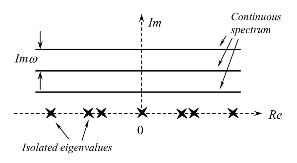
Figure 1: Spectrum of $K_{0}(\omega)$

Here, $N=N_{1}\otimes\mathchoice{\rm 1\mskip-4.0mul}{\rm 1\mskip-4.0mul}{\rm 1\mskip-4.5mul}{\rm 1\mskip-5.0mul}+\mathchoice{\rm 1\mskip-4.0mul}{\rm 1\mskip-4.0mul}{\rm 1\mskip-4.5mul}{\rm 1\mskip-5.0mul}\otimes N_{1}$ is the total number operator of a product of two bosonic Fock spaces ${\cal F}\otimes{\cal F}$ (the Gelfand-Naimark-Segal Hilbert space of the reservoir), and where $N_{1}$ is the usual number operator on $\mathcal{F}$. $N$ has spectrum ${\mathbb{N}}\cup\{0\}$, where $0$ is a simple eigenvalue (with vacuum eigenvector $\Omega_{{\rm R},\beta}=\Omega\otimes\Omega$). For real values of $\omega$, $U(\omega)$ is a group of unitaries. The spectrum of $K_{\lambda}(\omega)$ depends on ${\rm Im\,}\omega$ and moves according to the value of ${\rm Im\,}\omega$, whence the name “spectral deformation”. Even though $U(\omega)$ becomes unbounded for complex $\omega$, the r.h.s. of (3.10) is a well defined closed operator on a dense domain, analytic in $\omega$ at zero. Analyticity is used in the derivation of (3.9) and this is where the analyticity condition (A) after (3.2) comes into play. The operator $I(\omega)$ is infinitesimally small with respect to the number operator $N$. Hence we use perturbation theory in $\lambda$ to examine the spectrum of $K_{\lambda}(\omega)$.

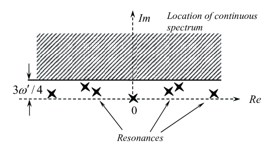
Figure 2: Spectrum of $K_{\lambda}(\omega)$. Resonances $\varepsilon_{e}^{(s)}$ are uncovered.

The point of the spectral deformation is that the (important part of the) spectrum of $K_{\lambda}(\omega)$ is much easier to analyze than that of $K_{\lambda}$, because the deformation uncovers the resonances of $K_{\lambda}$. We have (see Figure 1)

$${\rm spec\,}\big{(}K_{0}(\omega)\big{)}=\{E_{i}-E_{j}\}_{i,j=1,\ldots,N}\bigcup_{n\geq 1}\{\omega n+{\mathbb{R}}\},$$

because $K_{0}(\omega)=L_{0}+\omega N$, $L_{0}$ and $N$ commute, and the eigenvectors of $L_{0}=L_{\rm S}+L_{\rm R}$ are $\varphi_{i}\otimes\varphi_{j}\otimes\Omega_{{\rm R},\beta}$. Here, we have $H_{\rm S}\varphi_{j}=E_{j}\varphi_{j}$. The continuous spectrum is bounded away from the isolated eigenvalues by a gap of size ${\rm Im\,}\omega$. For values of the coupling parameter $\lambda$ small compared to ${\rm Im\,}\omega$, we can follow the displacements of the eigenvalues by using analytic perturbation theory. (Note that for ${\rm Im\,}\omega=0$, the eigenvalues are imbedded into the continuous spectrum, and analytic perturbation theory is not valid! The spectral deformation is indeed very useful!)

Theorem 3.2 ([19])

(See Fig. 2.) Fix ${\rm Im\,}\omega$ s.t. $0<{\rm Im\,}\omega<\omega^{\prime}$ (where $\omega^{\prime}$ is as in Condition (A)). There is a constant $c_{0}>0$ s.t. if $|\lambda|\leq c_{0}/\beta$ then, for all $\omega$ with ${\rm Im\,}\omega>7\omega^{\prime}/8$, the spectrum of $K_{\lambda}(\omega)$ in the complex half-plane $\{{\rm Im\,}z<\omega^{\prime}/2\}$ is independent of $\omega$ and consists purely of the distinct eigenvalues

$$\{\varepsilon_{e}^{(s)}\ :\ e\in{\rm spec}(L_{\rm S}),s=1,\ldots,\nu(e)\},$$

where $1\leq\nu(e)\leq{\rm mult}(e)$ counts the splitting of the eigenvalue $e$. Moreover,

$$\lim_{\lambda\rightarrow 0}|\varepsilon_{e}^{(s)}(\lambda)-e|=0$$

for all $s$, and we have ${\rm Im\,}\varepsilon_{e}^{(s)}\geq 0$. Also, the continuous spectrum of $K_{\lambda}(\omega)$ lies in the region $\{{\rm Im\,}z\geq 3\omega^{\prime}/4\}$.

Next we separate the contributions to the path integral in (3.9) coming from the singularities at the resonance energies and from the continuous spectrum. We deform the path of integration $z={\mathbb{R}}-{\rm i}$ into the line $z={\mathbb{R}}+{\rm i}\omega^{\prime}/2$, thereby picking up the residues of poles of the integrand at $\varepsilon_{e}^{(s)}$ (all $e$, $s$). Let ${\mathcal{C}}_{e}^{(s)}$ be a small circle around $\varepsilon_{e}^{(s)}$, not enclosing or touching any other spectrum of $K_{\lambda}(\omega)$. We introduce the generally non-orthogonal Riesz spectral projections

$$Q_{e}^{(s)}=Q_{e}^{(s)}(\omega,\lambda)=-\frac{1}{2\pi{\rm i}}\int_{{\mathcal{C}}_{e}^{(s)}}(K_{\lambda}(\omega)-z)^{-1}{\rm d}z.$$ (3.11)

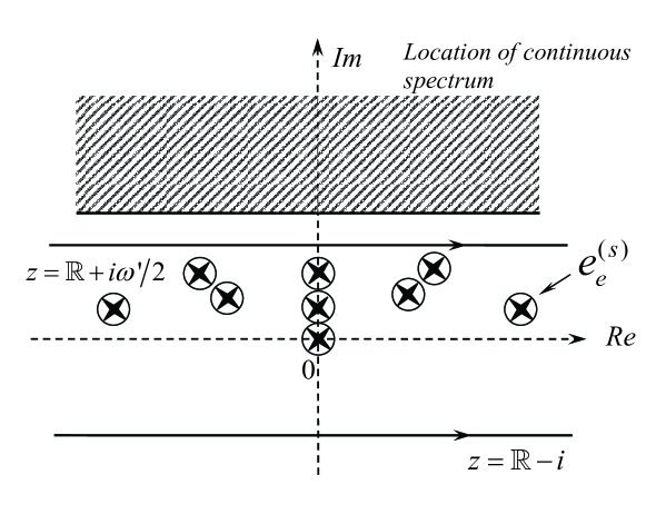
Figure 3: Contour deformation: $\int_{{\mathbb{R}}-{\rm i}}{\rm d}z=\sum_{e,s}\int_{{\mathcal{C}}_{e}^{(s)}}{\rm d}z+\int_{{\mathbb{R}}+{\rm i}\omega^{\prime}/2}{\rm d}z$

It follows from (3.9) that

$$\langle A\rangle_{t}=\sum_{e}\sum_{s=1}^{\nu(e)}{\rm e}^{{\rm i}t\varepsilon^{(s)}_{e}}\left\langle{\psi_{0}},{Q_{e}^{(s)}[A\otimes\mathchoice{\rm 1\mskip-4.0mul}{\rm 1\mskip-4.0mul}{\rm 1\mskip-4.5mul}{\rm 1\mskip-5.0mul}_{\rm S}\otimes\mathchoice{\rm 1\mskip-4.0mul}{\rm 1\mskip-4.0mul}{\rm 1\mskip-4.5mul}{\rm 1\mskip-5.0mul}_{\rm R}]\psi_{0}}\right\rangle+O(\lambda^{2}{\rm e}^{-\omega^{\prime}t/2}).$$ (3.12)

Note that the imaginary parts of all resonance energies $\varepsilon_{e}^{(s)}$ are smaller than $\omega^{\prime}/2$, so that the remainder term in (3.12) is not only small in $\lambda$, but it also decays faster than all of the terms in the sum. (See also Figure 3.) We point out also that instead of deforming the path integration contour as explained before (3.11), we could choose $z={\mathbb{R}}+{\rm i}[\omega^{\prime}-O(\lambda)]$, hence transforming the error term in (3.12) into the one given in (3.5).

Finally, we notice that all terms in (3.12) with $\varepsilon_{e}^{(s)}\neq 0$ will vanish in the ergodic mean limit, so

$$\langle\!\langle A\rangle\!\rangle_{\infty}=\lim_{T\rightarrow\infty}\frac{1}{T}\int_{0}^{T}\langle A\rangle_{t}\ {\rm d}t=\sum_{s:\varepsilon_{0}^{(s)}=0}\left\langle{\psi_{0}},{Q_{0}^{(s)}[A\otimes\mathchoice{\rm 1\mskip-4.0mul}{\rm 1\mskip-4.0mul}{\rm 1\mskip-4.5mul}{\rm 1\mskip-5.0mul}_{\rm R}\otimes\mathchoice{\rm 1\mskip-4.0mul}{\rm 1\mskip-4.0mul}{\rm 1\mskip-4.5mul}{\rm 1\mskip-5.0mul}_{\rm R}]\psi_{0}}\right\rangle.$$

We now see that the linear functionals (2.11) are represented as

$$R_{\varepsilon_{e}^{(s)}}(A)=\left\langle{\psi_{0}},{Q_{e}^{(s)}[A\otimes\mathchoice{\rm 1\mskip-4.0mul}{\rm 1\mskip-4.0mul}{\rm 1\mskip-4.5mul}{\rm 1\mskip-5.0mul}_{\rm S}\otimes\mathchoice{\rm 1\mskip-4.0mul}{\rm 1\mskip-4.0mul}{\rm 1\mskip-4.5mul}{\rm 1\mskip-5.0mul}_{\rm R}]\psi_{0}}\right\rangle.$$ (3.13)

This concludes the outline of the proof of Theorem 3.1.

References

• [1] Altepeter, J.B., Hadley, P.G., Wendelken, S.M., Berglund, A.J., Kwiat, P.G.: Experimental Investigation of a Two-Qubit Decoherence-Free Subspace. Phys. Rev. Lett. 92, no.14, 147901
• [2] Breuer, H.-P., Petruccione, F., The theory of open quantum systems. Oxford University Press 2002
• [3] Berman, G.P., Kamenev, D.I., Tsifrinovich, V.I.: Collective decoherence of the superpositional entangled states in the quantum Shor algorithm. Phys. Rev. A 71, 032346 (2005)
• [4] Clerk, A.A., Devoret, M.H., Girvin, S.M., Marquardt, F., and Schoelkopf, R.J.: Introduction to quantum noise, measurement and amplifcation. Preprint arXiv:0810.4729v1 [cond-mat] (2008).
• [5] Davies, E.B.: Markovian master equations. Comm. Math. Phys. 39, 91 (1974)
• [6] Davies, E.B.: Markovian Master Equations. II Math. Ann. 219, 147-158 (1976)
• [7] Dalvit, D.A.R., Berman, G.P., Vishik, M.: Dynamics of bosonic quantum systems in coherent state representation. Phys. Rev. A, 73, 013803 (2006)
• [8] Devoret, M.H. and Martinis, J.M.: Implementing qubits with superconducting integrated circuits. Quantum Information Processing 3, 163-203 (2004).
• [9] Dereziński, J., Früboes, R.: Fermi Golden Rule and Open Quantum Systems, in Lecture Notes in Mathematics 1882, Springer Verlag 2006
• [10] Duan, L.-M., Guo, G.-C.: Reducing decoherence in quantum-computer memory with all quantum bits coupling to the same environment. Phys. Rev. A 57, no.2, 737-741 (1998)
• [11] Fedorov, A., Fedichkin, L.: Collective decoherence of nuclear spin clusters. J. Phys. Condens. Matter 18, 3217-3228 (2006)
• [12] Jaks̆ić, V., Pillet, C.-A.: From resonances to master equations Ann. Inst. Henri Poincaré 67, no.4, 425-445 (1997)
• [13] Joos, E., Zeh, H.D., Kiefer, C., Giulini, D., Kupsch, J. Stamatescu, I.O.: Decoherence and the appearence of a classical world in quantum theory. Second edition. Springer Verlag, Berlin, 2003
• [14] Katz, N., Neeley, M., Ansmann, M., Bialczak, R.C., Hofheinz, M., Lucero, E., O’Connell, A.: Reversal of the weak measurement of a quantum state in a superconducting phase qubit. Phys. Rev. Lett. 101, 200401-1-4 (2008).
• [15] Kinion, D. and Clarke, J.: Microstrip superconducting quantum interference device radio-frequency amplifier: Scattering parameters and input coupling. Appl. Phys. Lett. 92, 172503 (2008)
• [16] Makhlin, Y., Schön, G., and Shnirman, A.: Quantum-state engineering with Josephson-junction devices. Rev. Mod. Phys.73, 380-400 (2001).
• [17] Merkli, M.: Level shift operators for open quantum systems. J. Math. Anal. Appl. 327, no. 1, 376–399 (2007)
• [18] Merkli, M., Sigal, I.M., and G.P. Berman, G.P.: Decoherence and Thermalization. Phys. Rev. Lett. 98, 130401 (2007).
• [19] Merkli, M., Sigal, I.M., and Berman, G.P.: Resonance theory of decoherence and thermalization. Annals of Physics 323, 373 (2008).
• [20] Merkli, M., Berman, B.P., and Sigal, I.M. :Dynamics of collective decoherence and thermalization. Annals of Physics 323, 3091 (2008).
• [21] Merkli, M., Mück, M., Sigal, I.M.: Instability of Equilibrium States for Coupled Heat Reservoirs at Different Temperatures. J. Funct. Anal. 243 no. 1, 87-120 (2007)
• [22] Mozyrsky, D., Privman, V.: Adiabatic Decoherence. Journ. Stat. Phys. 91, 3/4, 787-799 (1998)
• [23] Palma, G.M., Suominen, K.-A., Ekert, A.K.: Quantum Computers and Dissipation. Proc. R. Soc. Lond. A 452, 567-584 (1996)
• [24] Shao, J., Ge, M.-L., Cheng, H.: Decoherence of quantum-nondemolition systems. Phys. Rev. E, 53, no.1, 1243 - 1245 (1996)
• [25] Steffen, M., Ansmann, M., McDermott, R., Katz, N., Bialczak, R.C., Lucero, E., Neeley, M., Weig, E.M., Cleland, A.N. and Martinis, J.M.: State tomography of capacitively shunted phase qubits with high fidelity. Phys. Rev. Lett. 97 050502-1-4 (2006).
• [26] Wendin, G., and Shumeiko, V. S.: Quantum bits with Josephson junctions. (Review Article), Low Temp. Phys. 33, 724 (2007).
• [27] Yu, Y., Han, S., Chu, X., Chu, S.I., Wang, Z.: Coherent temporal oscillations of macroscopic quantum states in a Josephson junction, SCIENCE 296, 889-892 (2002).