A-D-E Classification of Conformal Field Theories

Andrea CAPPELLI

INFN
Via G. Sansone 1, 50019 Sesto Fiorentino (Firenze), Italy

Jean-Bernard ZUBER

LPTHE, Tour 24-25, 5ème étage,
Université Pierre et Marie Curie –- Paris 6,
4 Place Jussieu, F 75252 Paris Cedex 5, France

The ADE classification scheme is encountered in many areas of mathematics, most notably in the study of Lie algebras. Here such a scheme is shown to describe families of two-dimensional conformal field theories.

Review article to appear in Scholapedia, http://www.scholarpedia.org/

1 Overview

Conformal Field Theories (CFT) in two space-time dimensions have been the object of intensive work since the mid eighties, after the fundamental paper [1]. These theories have very diverse and important physical applications, from the description of critical behavior in statistical mechanics and solid state physics in low dimension, to the worldsheet description of string theory. Furthermore, their remarkable analytical and algebraic structures and their connections with many other domains of mathematics make them outstanding laboratories of new techniques and ideas. A particularly striking feature is the possibility of classifying large classes of CFT through the study of representations of the Virasoro algebra of conformal transformations [CFT].

The classification of CFT partition functions, leading to the ADE scheme, follows from exploiting the additional symmetry under modular transformations, the discrete coordinate changes that leave invariant the double-periodic finite-size geometry of the torus.

Modular invariance has a precursor in ordinary statistical mechanics of lattice models, like the Ising model [Ising]. Consider a finite $L\times T$ square lattice in two dimensions as in Fig.1: it is common to use the transfer matrix formalism to compute the partition function and other quantities of physical relevance in the model. Each configuration of degrees of freedom on a row of the lattice is associated with a state vector in a Hilbert space. The transfer matrix ${\bf T}_{H}$ is an operator acting on a state vector and manufacturing the state vector of the next row. It may thus be regarded as a discrete version of a time evolution operator, for time flowing vertically, see Fig. 1. The partition function of a system with $T$ rows and periodic boundary conditions in the time direction is then $Z={\rm tr}{\bf T}_{H}^{T}$. Now the model also admits a transfer matrix ${\bf T}_{V}$ in the orthogonal direction, (a column-to-column transfer matrix) and if periodic boundary conditions are also imposed in that direction, one has an alternative expression of the partition function: $Z={\rm\,{\rm Tr\,}}{\bf T}_{V}^{L}$. Therefore, in the doubly-periodic toroidal geometry there are two ways of writing the partition function. Imposing their equality may give some useful informations on the model, but in general these are too weak to constraint its operator content, spectrum, etc.

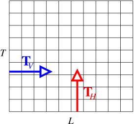
Figure 1: Two transfer matrices of a statistical lattice model.

In the case of conformal field theories, there are special features that allow for a complete solution of the modular invariance conditions [CFT]:

• The spectrum of states in the theory, is organized in families, the “conformal towers”, with an infinite dimensional algebra acting as a spectrum generating algebra, (the Virasoro algebra or one of its extensions [Vir]) [1]. The structure of these conformal towers is given by the representation theory of the “chiral” algebra parameterized by the Virasoro central charge $c$ and other quantum numbers.

• the Hamiltonian can be expressed in terms of the Virasoro generator of dilatations $L_{0}$ and its conjugate $\bar{L}_{0}$, whose eigenvalues give the conformal weights (scale dimensions). The lowest-energy state in each tower, i.e. in each Virasoro representation, is called the “highest weight vector” with conformal weight $h$ and the excited states are obtained by acting on it with algebra generators. (Note the mismatch of terminology: the highest weight vector is actually the lowest energy state.) The structure of each tower is encoded in the character of the representation, $\chi_{h}(q)$, which is the generating function of the dimensions of eigenspaces of given energy (see below eq. (5)).

• The partition function $Z$ can be rewritten in terms of the Hamiltonian and thus of the Virasoro generators $L_{0},\bar{L}_{0}$, (eq. (3) hereafter). As a consequence, it involves a sum of bilinears of characters with undetermined non negative integer multiplicities of representations in the theory, see eq. (6).

• The requirement of modular invariance constrains these multiplicities and allows for the complete classification of partition functions in some theories for which that character expansion of $Z$ is finite.

In this contribution, we describe this classification program in the simplest classes of conformal theories, namely the Virasoro minimal models, having central charge $c<1$, and the models with the affine Lie algebra $\widehat{sl}(2)$ as an extended symmetry. The main result is that the modular invariant partition functions are in one-to-one correspondence with the Dynkin diagrams of the A, D and E types [2]. Each partition function defines an independent theory with specific Hilbert space and field content.

2 Modular invariant partition functions

Two-dimensional conformal field theories are quantum field theories enjoying covariance properties under conformal, i.e. local scale, transformations [CFT]. It is postulated that such theories exist and are consistent on any two-dimensional Riemann surface [Ver]. In the case of the plane with complex coordinate $z$, one shows that $z$ and its complex conjugate $\bar{z}$ may be treated as independent variables, called holomorphic and anti-holomorphic coordinates. Infinitesimal conformal transformations are generated by two copies of the Virasoro algebra [Vir], acting on $z$ and $\bar{z}$ and called right and left chiral algebras, respectively. More generally, one may consider theories with an extended chiral algebra ${\cal A}$ containing Virasoro, such as the affine Lie (Kac–Moody) algebras [KM], the superconformal algebras, etc. The Hilbert space ${\cal H}$ of the CFT decomposes onto pairs of representations ${\cal V}_{j}$ of the left and right copies of the Virasoro algebra or of ${\cal A}$. For “rational” conformal field theories (RCFT), the number of such irreducible representations ${\cal V}_{j}$ is finite. We label by $j\in{\cal I}$ and $\bar{\jmath}\in{\cal I}$ the left and right irreducible representations, respectively. These pairs of representations are in one-to-one correspondence with the “primary conformal fields” $\phi_{j\bar{\jmath}}$ [CFT].

The finite decomposition of the RCFT Hilbert space can be written:

$${\cal H}=\oplus_{j\bar{\jmath}\in{\cal I}}\ N_{j\bar{\jmath}}\ {\cal V}_{j}\otimes{\cal V}_{\bar{\jmath}}\ ,$$ (1)

where $N_{j\bar{\jmath}}$ are non negative integer multiplicities. These are subjected to consistency constraints, due to the fact that the RCFT must exist and be consistent on any Riemann surface [Ver]. In particular, a crucial condition on the torus is the modular invariance of the partition function: this requirement determines the $N_{j\bar{\jmath}}$ as described hereafter.

We start by considering the theory defined on a cylinder (see Fig.2) of perimeter $L$ with a coordinate $w$; points of coordinates $w$ and $w+L$ are identified. This cylinder is equivalent to the plane punctured at the origin, equipped with a complex coordinate $z$, by means of the conformal mapping $z=\exp(-2\pi iw/L)$. On the cylinder, it is natural to think of the Hamiltonian as the operator of translation along its axis (the imaginary axis in $w$), or more generally along any helix, defined by its complex period $\tau L$ in the $w$ plane, with $\Im m\,\tau>0$: ${\tau=iT/L}$ in the particular case of Fig.1, while the general case is depicted in Fig. 3. The Virasoro generators of translations in $w$ and $\bar{w}$ (regarded as independent variables) are identified with $L_{-1}^{{\rm cyl}}$ and $\bar{L}_{-1}^{{\rm cyl}}$, therefore $H^{{\rm cyl}}=\tau L_{-1}^{{\rm cyl}}+\bar{\tau}\bar{L}_{-1}^{{\rm cyl}}$, with $\bar{\tau}$ the complex conjugate of $\tau$.

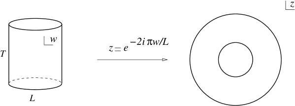
Figure 2: Mapping from the cylinder to the annulus in the punctured plane: the two edges are identified for periodic boundary conditions, while they are left independent in boundary CFT described in Section 4.

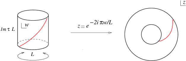
Figure 3: Time evolution on the cylinder along an helix, and its image in the annulus.

Through the conformal mapping $w\mapsto z$, it is clear that these translations correspond to dilatations and rotations in the plane. Indeed, using the transformation law of the energy-momentum tensor, one finds [BCFT]:

$${L_{-1}^{{\rm cyl}}=-{2\pi i\over L}(L_{0}-{c\over 24})}\ ,$$ (2)

where $L_{0}$ belongs to the Virasoro algebra of the plane and the term $c/24$ comes from the conformal anomaly. In the continuum formulation, the transfer matrix is the exponential of the Hamiltonian, ${\bf T}=\exp(-\Delta t\ H)$ and therefore, the evolution operator on a cylinder of length $(\Im m\,\tau)L$ is given by:

$$\exp\left(-H^{\rm cyl}L\right)=\exp\left[2\pi i\tau\left(L_{0}-{c\over 24}\right)-2\pi i\bar{\tau}\left(\bar{L}_{0}-{c\over 24}\right)\right]\ .$$ (3)

We now introduce the partition function of the theory on a torus $\mathbb{T}$: this is expressed by the trace of the evolution operator, owing to the identification of the two ends of the cylinder,

$$Z\left(\tau\right)=\,{\rm Tr\,}_{{\cal H}}\ e^{2\pi i[\tau(L_{0}-{c\over 24})-\bar{\tau}(\bar{L}_{0}-{c\over 24})]}\ .$$ (4)

Each irreducible representation ${\cal V}_{j}$ of Vir (or of ${\cal A}$) is graded for the action of the Virasoro generator $L_{0}$: the spectrum of $L_{0}$ in ${\cal V}_{j}$ is of the form $\{h_{j},h_{j}+1,h_{j}+2,\cdots\}$, with non-trivial multiplicities $m_{n}=\dim$(subspace of eigenvalue $h_{j}+n$). It is thus natural to introduce a generating function of these multiplicities, i.e. a function of a dummy variable $q$, called the character of the representation ${\cal V}_{j}$:

$$\chi_{j}(q)=\,{\rm Tr\,}_{{\cal V}_{j}}\ q^{L_{0}-{{c\over 24}}}=q^{h_{j}-{{c\over 24}}}\sum_{n=0}^{\infty}m_{n}q^{n}\ .$$ (5)

These functions have been computed for several classes of chiral algebras [4].

Using (1) and the definition of characters, the trace in (4) may be written as:

$$Z\left(\tau\right)=\sum_{j{\bar{\jmath}}}\ N_{j{\bar{\jmath}}}\ \chi_{j}(q)\ \chi_{\bar{\jmath}}(\bar{q})\ ,\qquad\qquad q=e^{2\pi i\tau}\ ,\quad\bar{q}=e^{-2\pi i\bar{\tau}}\ .$$ (6)

Let’s stress that in these expressions, $\bar{q}$ is the complex conjugate of $q$, and therefore, $Z$ is a sesquilinear form in the characters. Equation (6) shows that the torus partition function provides a convenient way of encoding the structure of the RCFT Hilbert space (1).

The geometry of the torus $\mathbb{T}$ has been specified in (6) through the modular parameter $\tau$, $\Im m\,\tau>0$; the two periods are $1$ and $\tau$, up to a global, irrelevant dilatation by $L$. Equivalently, the torus may be regarded as the quotient of the complex $w$-plane by the lattice generated by the two numbers $1$ and $\tau$:

$$\mathbb{T}=\mathbb{C}/(\mathbb{Z}\oplus\tau\mathbb{Z})\ ,$$ (7)

in the sense that points are identified according to $w\sim w^{\prime}=w+n+m\tau$, $n,m\in\mathbb{Z}$. This shows that there is a redundancy in the description of the torus: the modular parameters $\tau$ and $(c+d\tau)/(a+b\tau)$ describe the same torus, for any transformation of the modular group: $M=\left({a\ b\atop c\ d}\right)\in PSL(2,\mathbb{Z})$, with $a,b,c,d\in\mathbb{Z}$ defined up to a global sign and satisfying $ad-bc=1$. The group is generated by the two transformations: $T:\tau\to\tau+1$ and $S:\tau\to-1/\tau$ [3]: the first one is depicted in Fig.4 and the second exchanges the two periods of the torus generalizing the case in Fig.1.

The partition function must be uniquely defined on the torus, independently of coordinate choices, and thus be invariant under modular transformations:

$$Z\left(-\frac{1}{\tau}\right)=Z\left(\tau+1\right)=Z\left(\tau\right)\ .$$ (8)

These conditions, together with the expression (6) of $Z$ as a sesquilinear form in the characters, were introduced by Cardy [5]. As we shall show in the following, they open a route to the classification of RCFTs.

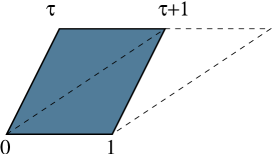
Figure 4: Elementary cell in the $w$-plane describing the torus. The $T$ modular transformation leads to the equivalent cell with parameter $\tau^{\prime}=\tau+1$.

In RCFTs, the finite set of characters $\chi_{j}$, $j\in{\cal I}$, transforms under modular transformations according to a unitary linear representation. It suffices to give the action of the two generators of the modular group acting on $\tau$, hence on $q=\exp 2\pi i\tau$,

$$\tau\mapsto\tau^{\prime}=\tau+1\ ,\qquad \chi_{j}(q^{\prime})=e^{2\pi i(h_{j}-\frac{c}{24})}\chi_{j}(q)=\sum_{j^{\prime}\in{\cal I}}T_{jj^{\prime}}\ \chi_{j^{\prime}}(q)\ ,$$ (9)

$$\tau\mapsto\tau^{\prime}=-\frac{1}{\tau}\ ,\qquad\quad \chi_{j}(q^{\prime})=\sum_{j^{\prime}\in{\cal I}}S_{jj^{\prime}}\ \chi_{j^{\prime}}(q)\ ;$$ (10)

$T$ and $S$ are unitary matrices [Ver]. It follows that RCFT partition functions (6) are modular invariant if the (non-negative) integer multiplicity matrices $N_{j{\bar{\jmath}}}$ obey the conditions:

$$SNS^{\dagger}=TNT^{\dagger}=N\ .$$ (11)

When explicit computations of the partition function (path integral) are possible, the results should automatically be modular invariant. In case of the strongly-interacting RCFTs, such derivations are not usually available: one can consider the algebraic construction described here, starting from the representations of the chiral algebra, and impose the modular invariance condition. Let us stress that in this approach, modular invariance of $Z$ is just one necessary condition for the consistency of the theory: there are additional requirements on other quantities, such as the crossing symmetry of the four-point function on the plane [1] [6] (See [Ver]).

3 A-D-E Classification

We thus are led to the following:
Classification Problem. For a given chiral algebra, find all possible Hilbert spaces (1), i.e. all possible sesquilinear forms (6) with non negative integer coefficients that are modular invariant, and such that $N_{11}=1$.

The label $1$ refers to the identity representation (with $h_{1}=0$) and the condition $N_{11}=1$ expresses the unicity of the ground state. As mentioned above, the finite set of characters of any RCFT, labelled by ${\cal I}$, supports a unitary representation of the modular group. This implies that the diagonal combination of characters, $Z=\sum_{i\in{\cal I}}\chi_{i}(q)\overline{\chi_{i}(q)}$, is always modular invariant for any RCFT.

Finding the general solutions for $Z$ in any RCFT is a well posed, although involved, algebraic problem. Complete results are known in a few cases, in particular in several families of RCFT’s based on the $sl(2)$ algebra, for which a special feature, the ADE classification, emerges.

$$\begin{array}[]{|c|c|c|}\hline\cr{\rm level}&Z&{\rm diagram}\\ \hline\cr\hline\cr k\geq 0&\displaystyle{\sum_{\lambda=1}^{k+1}\left|\chi_{\lambda}\right|^{2}}&A_{k+1}\\ \hline\cr k=4\rho\geq 4&\displaystyle{\sum^{2\rho-1}_{\lambda\ {\rm odd}\ =1}\left|\chi_{\lambda}+\chi_{4\rho+2-\lambda}\right|^{2}+2\left|\chi_{2\rho+1}\right|^{2}}&D_{2\rho+2}\\ \hline\cr k=4\rho-2\geq 6&\displaystyle{\sum^{4\rho-1}_{\lambda\ {\rm odd}\ =1}\left|\chi_{\lambda}\right|^{2}+\left|\chi_{2\rho}\right|^{2}+\sum_{\lambda\ {\rm even}=2}^{2\rho-2}\left(\chi_{\lambda}\overline{\chi}_{4\rho-\lambda}+{\rm c.c.}\right)}&D_{2\rho+1}\\ \hline\cr k=10&\displaystyle{\left|\chi_{1}+\chi_{7}\right|^{2}+\left|\chi_{4}+\chi_{8}\right|^{2}+\left|\chi_{5}+\chi_{11}\right|^{2}}&E_{6}\\ \hline\cr k=16&\begin{array}[]{c}\displaystyle{\left|\chi_{1}+\chi_{17}\right|^{2}+\left|\chi_{5}+\chi_{13}\right|^{2}+\left|\chi_{7}+\chi_{11}\right|^{2}+\left|\chi_{9}\right|^{2}}\\ \displaystyle{\qquad+\left[(\chi_{3}+\chi_{15})\overline{\chi}_{9}+{\rm c.c.}\right]}\end{array}&E_{7}\\ \hline\cr k=28&\displaystyle{\left|\chi_{1}+\chi_{11}+\chi_{19}+\chi_{29}\right|^{2}+\left|\chi_{7}+\chi_{13}+\chi_{17}+\chi_{23}\right|^{2}}&E_{8}\\ \hline\cr\end{array}$$

Table 1: List of modular invariant partition functions of $\widehat{sl}(2)$ RCFTs: $\chi_{\lambda}$ are characters of representations of the affine algebra at level $k$. The last column shows the associated ADE Dynkin diagram.

3.1 The $\widehat{sl}(2)$ cases.

For ${\cal A}=\widehat{sl}(2)$, the $sl(2)$ affine Kac-Moody algebra at a non negative integer value of the “level” $k$ (its central charge), the set of possible “integrable” representations is labelled by an integer or half-integer $j$ (the spin of the representation of the “horizontal algebra”), subject to $0\leq j\leq k/2$, or more conveniently by the integer $\lambda=2j+1$, $1\leq\lambda\leq k+1$ [KM]. The matrix of modular transformations in (10) reads:

$$S_{\lambda\lambda^{\prime}}=\left(\frac{2}{k+2}\right)^{1/2}\sin\left(\frac{\pi\lambda\lambda^{\prime}}{k+2}\right)\ ,$$ (12)

the Virasoro central charge and the conformal weights are,

$$c=\frac{3k}{k+2}\ ,\qquad\quad h_{\lambda}=\frac{\lambda^{2}-1}{4(k+2)}\ .$$ (13)

$G$	diagram	$h$	exponents $\ell_{n}$
$A_{n}$		$n+1$	$1,2,\cdots,n$
$D_{n+2}$		$2(n+1)$	$1,3,\cdots,2n+1,n+1$
$E_{6}$		12	$1,4,5,7,8,11$
$E_{7}$		18	$1,5,7,9,11,13,17$
$E_{8}$		30	$1,7,11,13,17,19,23,29$

Table 2: ADE Dynkin diagrams with Coxeter numbers $h$ and exponents $\ell_{n}$.

The study of modular invariance of partition functions leads to the determination of all possible matrices $N_{\lambda,\bar{\lambda}}$ in (6); they are displayed in Table 1. The result was first conjectured in [7] and then proved in [8], [9]; partial results had been previously obtained by several authors, including [5] and [10]. The analysis was made in two steps: i) the derivation of the complete list of sesquilinear invariants forms irrespectively of the positivity of their coefficients; ii) the imposition of positivity. The proof is rather long and cannot be described here: let us just give a clue. Given that the $S$ matrix is a discrete Fourier transform, one is dealing with the algebra of numbers $\lambda$ defined modulo $n=2(k+2)$: one finds that there is one independent modular invariant for each number $\omega$ solution of $\omega^{2}=1$ mod $2n$ [7] [11]. It is given by a sort of permutation matrix, $N_{\lambda,\lambda^{\prime}}=\delta_{\lambda,\omega\lambda^{\prime}\ {\rm mod}\ n}$, that obeys the conditions (11). The range of indices of the characters, however, is only $n/2$ rather than $n$, with the following periodicity property: $\chi_{\lambda}=-\chi_{\lambda+n/2}=\chi_{\lambda+n}$; therefore, most of these solutions actually correspond to sesquilinear forms (6) with some negative coefficients. A deeper analysis then obtained the subset of positive definite ones that are shown in Table 1 [8]. More recently, a simpler method was found that directly searches for the positive invariants [12].

The list of modular invariants in Table 1 exhibits a remarkable feature: a one-to-one correspondence with the ADE Dynkin diagrams, which are best known for the classification of simply-laced simple Lie algebras (See Table 2) [2]. The relation is as follows: if we analyze the diagonal terms of expressions in Table 1, their labels $\lambda$ turn out to be the “Coxeter exponents” $\ell_{n}$ of the Dynkin diagrams; these are given in Table 2 and will be defined shortly. For example, in the $E_{7}$ modular invariant of Table 1, the diagonal terms are labelled by odd integers from 1 to 17, excluding 3 and 15, which matches the $E_{7}$ exponents of Table 2. Moreover, the Coxeter number $h$, another characteristic of the diagrams, is related to the $\widehat{sl}(2)$ level by $h=k+2$.

We recall that the Dynkin diagrams encode the geometry of root systems $\{\alpha_{a}\}$ of simple Lie algebras [2]: the simply-laced ones have roots of equal length and the Cartan matrix, $C_{ab}=(\alpha_{a},\alpha_{b})$, is expressed in terms of the adjacency matrix $G$ of the diagram, $C_{ab}=2I-G_{ab}$ (the matrix $G$ is defined for any graph as $G_{ab}=1$ if sites $(a,b)$ are connected and zero otherwise). For these diagrams, the eigenvalues of the adjacency matrix $G$ are of the form $2\cos(\pi\ell_{n}/h)$, where $h$ is the Coxeter number, and $\ell_{n}$ the Coxeter exponents. These numbers take rank($G$) values (the number of vertices of $G$), ranging between $1$ and $h-1$, with possible multiplicities. The exponents also express other properties: for example, when shifted by $1$, they give the degrees of all invariant polynomials of the Lie algebra: the quadratic Casimir invariant ($\ell=1$) and the higher invariants ($\ell>1$). The Coxeter number and exponents are listed in Table 2.

3.2 Minimal conformal models

The “minimal models” introduced in Ref [1] are the only RCFT with values $c<1$ of the central charge of the Virasoro algebra:

$$c\left(p,p^{\prime}\right)=1-\frac{6(p-p^{\prime})^{2}}{pp^{\prime}}\ ,\qquad p,p^{\prime}\in\mathbb{Z}^{+},\quad(p,p^{\prime})=1,$$ (14)

($p$ and $p^{\prime}$ are positive coprime integers). The highest weights of representations take values in the “Kac table” [CFT]:

$$h_{rs}=\frac{(rp-sp^{\prime})^{2}-(p-p^{\prime})^{2}}{4pp^{\prime}},\qquad 1\leq r\leq p^{\prime}-1\ ,\quad 1\leq s\leq p-1\ ,$$ (15)

quotiented by the equivalence $(r,s)\sim(p^{\prime}-r,p-s)$. In Ref [7], the partition functions of minimal models were shown to also follow the ADE scheme: the results are displayed in Table 3. In this case, the partition functions are associated to pairs of diagrams: one of them is always of the $A$ type, because one of the Coxeter numbers $(p,p^{\prime})$ is odd. Besides the diagonal invariants, there are two infinite series, $(D,A_{p-1})$ and $(A_{p^{\prime}-1},D)$, and six exceptional cases, $(E,A)$, $(A,E)$. The similarity between the two ADE classifications can be traced back to the relation between Virasoro representations and affine $\widehat{sl}(2)$ algebra representations [KM], given by the coset construction: ${\rm Vir}\sim\widehat{sl}(2)_{p^{\prime}}\otimes\widehat{sl}(2)_{p-p^{\prime}}/\widehat{sl}(2)_{p}$ (for $p=p^{\prime}+1$) [13][4].

$$\begin{array}[]{|c|c|c|}\hline\cr p^{\prime}&Z&{\rm diagrams}\\ \hline\cr\hline\cr&\displaystyle{\frac{1}{2}\sum_{r=1}^{p^{\prime}-1}\sum_{s=1}^{p-1}\left|\chi_{rs}\right|^{2}}&(A_{p^{\prime}-1},A_{p-1})\\ \hline\cr\displaystyle{p^{\prime}=4\rho+2\atop\rho\geq 1}&\displaystyle{\frac{1}{2}\sum_{s=1}^{p-1}\left\{\sum^{2\rho-1}_{r\ {\rm odd}\ =1}\left|\chi_{r,s}+\chi_{4\rho+2-r,s}\right|^{2}+2\left|\chi_{2\rho+1,s}\right|^{2}\right\}}&(D_{2\rho+2},A_{p-1})\\ \hline\cr\displaystyle{{p^{\prime}=4\rho\atop\rho\geq 2}}&\displaystyle{\frac{1}{2}\sum_{s=1}^{p-1}\left\{\sum^{4\rho-1}_{r\ {\rm odd}\ =1}|\chi_{r,s}|^{2}+|\chi_{2\rho,s}|^{2}+\sum_{r\ {\rm even}=2}^{2\rho-2}\left(\chi_{r,s}\overline{\chi}_{4\rho-r,s}+{\rm c.c.}\right)\right\}}&(D_{2\rho+1},A_{p-1})\\ \hline\cr p^{\prime}=12&\displaystyle{\frac{1}{2}\sum_{s=1}^{p-1}\left\{\left|\chi_{1,s}+\chi_{7,s}\right|^{2}+\left|\chi_{4,s}+\chi_{8,s}\right|^{2}+\left|\chi_{5,s}+\chi_{11,s}\right|^{2}\right\}}&(E_{6},A_{p-1})\\ \hline\cr p^{\prime}=18&\displaystyle{\frac{1}{2}\sum_{s=1}^{p-1}\left\{\left|\chi_{1,s}+\chi_{17,s}\right|^{2}+\left|\chi_{5,s}+\chi_{13,s}\right|^{2}+\left|\chi_{7,s}+\chi_{11,s}\right|^{2}+\left|\chi_{9,s}\right|^{2}\right.}\atop\displaystyle{\left.\qquad+\left[\left(\chi_{3,s}+\chi_{15,s}\right)\overline{\chi}_{9,s}+{\rm c.c.}\right]\right\}}&(E_{7},A_{p-1})\\ \hline\cr p^{\prime}=30&\displaystyle{\frac{1}{2}\sum_{s=1}^{p-1}\left\{\left|\chi_{1,s}+\chi_{11,s}+\chi_{19,s}+\chi_{29.s}\right|^{2}+\left|\chi_{7,s}+\chi_{13,s}+\chi_{17,s}+\chi_{23,s}\right|^{2}\right\}}&(E_{8},A_{p-1})\\ \hline\cr\end{array}$$

Table 3: List of modular invariant partition functions of minimal models with $c(p,p^{\prime})<1$: $\chi_{r,s}$ are characters of Virasoro representations with highest weight $h_{rs}$ in (15). Each invariant, but the first, also occurs for $p\leftrightarrow p^{\prime}$.

The results in Table 3 amount to a classification of the operator contents of all rational conformal theories with $c<1$; we see that more than one consistent set of primary fields is possible for the same central charge (14), leading to quite different theories. These correspond to independent universality classes of critical phenomena in statistical mechanics, because the (relevant) primary fields characterize the manifold of perturbations around the fixed point. Let us mention some examples among the unitary minimal models corresponding to $(p,p^{\prime})=(m+1,m)$ or $(m,m+1)$, with $m=3,4,\dots$. In the $(A_{m-1},A_{m})$ series, the $(A_{2},A_{3})$ model is the Ising model, $(A_{3},A_{4})$ is the tricritical Ising and the higher models are their restricted solid-on-solid (RSOS) generalizations [14] [15] [16]. The simplest non-diagonal partition functions are: $(A_{4},D_{4})$ corresponding to the 3-state Potts model and $(D_{4},A_{6})$ its tricritical version [5].

Related ADE classifications of partition functions were found for the minimal superconformal theories [17], the $\mathbb{Z}_{k}$ parafermionic theories [11] and the ${\cal N}=2$ superconformal theories [18], all being connected with the $\widehat{sl}(2)$ affine algebra by coset constructions.

The classification of partition functions has also been completed for the case of the affine $\widehat{sl}(3)$ models [19]; the interpretation of the results in terms of generalized graphs has been considered in [20] [21]. Partial results have been obtained for other, higher rank algebras (for a review see [22]).

4 Partition functions on the annulus with boundary conditions

The ADE classification of modular invariants described in the previous section does not directly use, or relates to, properties of Lie algebras and the associated geometry of root lattices. However, a closer connection has been found in the corresponding classification of partition functions with a boundary [23].

As discussed in [BCFT], the partition function on the annulus (cf. Fig 2), with given conformal-preserving boundary conditions, is expressed in terms of the conformal characters (5) of a single chiral algebra:

$$Z_{a|b}(q)=\sum_{i\in\cal I}\ n_{ia}^{\ b}\ \chi_{i}(q)\ ,$$ (16)

where $q=\exp\left(-\pi L/T\right)$ in the notation of Fig.2. In this equation, the $a,b$ indices label the boundary conditions on the two edges of the annulus: as in the torus expansion (6), the integers $n_{ia}^{\ b}$ count the multiplicities of chiral representations pertaining to the Hilbert space of states compatible with the boundary conditions. In RCFTs, the number of boundary conditions is also finite, and a lot of information about the theory in the bulk may be obtained from the study of boundary states.

We also need to introduce the “fusion rules” and “fusion algebra” [Ver] [4]: they give the selection rules for the product of representations of chiral algebras of RCFTs, inherited from the operator product expansion of quantum field theory. It is natural to decompose the fusion of two representations labelled by $i,j\in{\cal I}$ into other representations, as follows:

$${\cal V}_{i}\bullet{\cal V}_{j}=\bigoplus_{k\in{\cal I}}\ {\cal N}_{ij}{}^{k}\ {\cal V}_{k}\ ,$$ (17)

thus defining the multiplicities, or “fusion coefficients”, ${\cal N}_{ij}{}^{k}$. Due to the properties of the operator product, the $({\cal N}_{i})_{j}^{\ k}$ matrices yield an associative and commutative algebra over the integer numbers called fusion algebra.

There is a remarkable formula, due to Verlinde [24][Ver], expressing these multiplicities in terms of the unitary modular matrix $S$ defined in (10):

$${\cal N}_{ij}{}^{k}=\sum_{\ell\in{\cal I}}\frac{S_{i\ell}\ S_{j\ell}\ \overline{S}_{k\ell}}{S_{1\ell}}\ .$$ (18)

This general result in RCFT follows from consistency conditions relating multipoint amplitudes on Riemann surfaces [6].

In the annulus geometry, the partition function can also be expressed in two alternative (and different) ways corresponding to evolutions in the two orthogonal directions (cf. Fig. 1), one of whose is (16). Their comparison yields Cardy’s equation of modular covariance on the annulus [BCFT] [25]. Supplemented by some technical assumptions of orthogonality and completeness of boundary conditions [26], this equation implies that the matrices of multiplicities, $n_{i}=\left(n_{i}\right)_{a}^{\ b}$, in (16) must form a representation of the fusion algebra,

$${n_{i}\;n_{j}=\sum_{k\in{\cal I}}{\cal N}_{ij}{}^{k}\,n_{k}\ }\ .$$ (19)

The study of (orthogonal complete) boundary conditions is thus given by the study of non-negative integer valued matrix representations (or “nimreps”) of the fusion algebra [23]. In the case of diagonal torus invariants, one actually has $(n_{i})_{j}^{\ k}=({\cal N}_{j})_{j}^{\ k}$, and there is a complete correspondence between the bulk and boundary sectors of the theory. For general, non-diagonal torus partition functions, one finds that the eigenvalues of $n_{i}$ are the same as those of ${\cal N}_{i}$, and are of the form $S_{ij}/S_{1j}$, owing to (18); however, the $j$ label can only take the values corresponding to the diagonal terms, for which $N_{jj}\neq 0$ in the expression of the torus partition function (6).

In the case of $\widehat{sl}(2)$ theories, the study of boundary conditions can be carried out completely. The fusion algebra is generated by the first non trivial matrix ${\cal N}_{2}$ (corresponding to spin $1/2$). From section 3.1, its eigenvalues are of the form $S_{2\ell}/S_{1\ell}=\sin(2\pi\ell/h)/\sin(\pi\ell/h)=2\cos(\pi\ell/h)$, thus in the interval $]-2,2[$. This property is shared by the matrix $n_{2}$ of multiplicities in (16), which also generates the whole set $\{n_{i}\}$. The study of boundary conditions thus reduces to finding all matrices $n_{2}$ with that spectral property.

A theorem (see [27]) states that the symmetric matrices with non negative integer entries and eigenvalues between $-2$ and $2$ are the adjacency matrices $G_{ab}$ of the ADE graphs of Table 2. Therefore, the ADE classification of $\widehat{sl}(2)$ theories, obtained through the imposition of their consistency on a torus, reappears through the consistency of their possible boundary conditions. In particular, the occurrence of Coxeter exponents as labelling diagonal terms in the torus partition functions receives a natural explanation (see Table 1). We remark that the same characterization of ADE graphs also occurs for the Cartan matrix in the classification of Lie algebras; this provides a more direct link between the two problems.

(For completeness, we observe that the set of $\widehat{sl}(2)$ boundary conditions, i.e. of fusion algebra representations, is not completely equivalent to that of torus partition functions. Actually, the theorem above provides additional fusion matrices $n_{2}$, associated to “tadpole” graphs $T_{n}=A_{2n}/\mathbb{Z}_{2}$ [23], but they do not correspond to any modular invariant $Z$. One can show by inspection that a multiplicity matrix $N_{\lambda\lambda^{\prime}}$ in (6), whose diagonal terms would be labelled by tadpole exponents, could not satisfy the invariance conditions (11). Still, the study of boundary conditions leads to a neat appearence of the ADE scheme.)

5 Physical realizations of A-D-E partition functions

There are two classes of CFTs for which the ADE classification appears from a more physical standpoint: the $c<1$ (unitary) minimal models, and the minimal ${\cal N}=2$ superconformal field theories ($c<3$) (and their topological cousins).

In the former case, the $c<1$ minimal models admit a realization as integrable statistical systems on a lattice [16]. In these solid-on-solid models, the patterns of heights are given by paths on a graph: by demanding that the configuration space supports a representation of the Temperley-Lieb algebra (a quantum deformation of the symmetric group algebra and a known way to achieve Yang-Baxter integrability [YB]) and that the model is at the critical point, one is led to graphs whose adjacency matrix has eigenvalues between $-2$ and $2$, hence of ADE type. This construction of minimal models was found at the same time of the classification of partition functions, thus providing a useful physical implementation of it. The lattice model based on a Dynkin diagram $G$ of ADE type, with Coxeter number $h$, is mapped in the continuum limit onto the minimal CFT with $(A_{h-2},G)$ modular invariant, while the $(G,A_{h})$ modular invariant describes a tricritical version of the same lattice model [28] [29] [30].

The minimal ${\cal N}=2$ superCFTs admit a Lagrangian description, involving chiral superfields and a holomorphic superpotential $W$ [31] [32]. Due to supersymmetry, the form of $W$ is protected by nonrenormalization theorems; therefore, the semiclassical Landau-Ginsburg theory [LG] of critical points as stationary points of the potential $W$ holds at the full quantum level. For example, the simpler $m$-th critical point is described in terms of a single chiral field $\Phi$ and the potential $W=\lambda\Phi^{m+1}$. A perturbation that moves the theory off the critical point and eventually lowers the degree of criticality is represented by:

$$W\left(\Phi\right)=\lambda\Phi^{m+1}+\mu_{k}\Phi^{k}\ ,\qquad k=1,\dots,m-1.$$ (20)

Indeed, the coupling $\mu_{k}\in[0,\infty]$ is relevant and describes the renormalization-group flow from the $m$-th critical point to the $(k-1)$-th one. The phase diagram around multicritical points is described by these perturbations that match Wilson’s analysis of relevant and marginal scaling fields; the higher the degree of criticality, the larger the number of these fields.

In this setting, one can make contact with another occurrence of the ADE scheme, that of Arnold’s singularities [33]. This is the study of critical points of polynomials $W(x_{1},x_{2},\cdots,x_{p})$, i.e. $\partial W/\partial x_{i}|_{0}=0$ for all $i=1,\cdots,p$, that are identified up to diffeomorphisms of the $x_{i}$ coordinates. As in (20), each singularity has an associated vector space of “genuine” deformations, that cannot be removed by reparametrizations: they may keep the same degree of the singularity or lower it, namely keep the vector space unchanged or reduce it, respectively. Deformations of the former type are called “moduli” and the “simple” singularities have none of them. A theorem states that simple singularities for any number $p$ of coordinates fall into the ADE scheme: they are actually given by the “Kleinian polynomials” $W$ that are listed in Table 4 (discarding the quadratic terms) ([33].

Arnold’s study of singularities can be used to classify the stationary points of Landau-Ginsburg potentials: the reparametrizations are redefinitions of the effective field(s) that have no physical effect, and the moduli are deformations preserving the critical degree, i.e. marginal perturbations. The simple singularities correspond to isolated critical points, that is, without marginal operators. Therefore, the ADE scheme classifies the isolated critical points of ${\cal N}=2$ Landau-Ginsburg superpotentials and matches the series of superconformal minimal models [31] [32]. This description applies to the “chiral sector” of the theory [18].

Let us notice that the classifications of ${\cal N}=2$ and ${\cal N}=0$ (Virasoro) minimal models are very similar: the former involve one ADE scheme (through the $\widehat{sl}(2)$ classification, Table 1), the second a double scheme (Table 3). Indeed, several results have shown that a qualitative Landau-Ginsburg description of Virasoro minimal models is possible, in spite of renormalization changing the conformal dimensions of fields [34] [35] ([36] discuss the case with boundaries). However, a detailed correspondence with ADE singularities cannot be found as in the supersymmetric case. Still the Landau-Ginsburg description, supplemented by the Arnold study of simple singularities, provides a qualitative physical picture for the ADE schemes found in the minimal CFTs.

We finally mention that rational CFTs find several applications in low-dimensional condensed-matter systems, like spin chains and quantum wires in $(1+1)$ dimensions [37] and quantum Hall effect in $(2+1)$ dimensions [38]. In the latter case in particular, modular invariant partition functions have been found in [39] [40] and the RCFT methods of section 4 have been exploited in [41].

$$\begin{array}[]{|c||ccccc|}\hline\cr\Gamma&{\cal C}_{n}&{\cal D}_{n}&{\cal T}&{\cal O}&{\cal I}\\ |\Gamma|&n&4n&24&48&120\\ W&X^{n}-YZ&X^{n+1}+XY^{2}+Z^{2}&X^{4}+Y^{3}+Z^{2}&X^{3}+XY^{3}+Z^{2}&X^{5}+Y^{3}+Z^{2}\\ G&A_{n-1}&D_{n+2}&E_{6}&E_{7}&E_{8}\\ \hline\cr\end{array}$$

Table 4: Finite subgroups $\Gamma$ of $SU(2)$, their orders $|\Gamma|$, the Kleinian polynomials $W$ and the associated Dynkin diagram. Arnold’s simple singularities are the polynomials without quadratic terms.

6 Elements of ADE-ology

The occurrence of the ADE scheme in the solution of modular invariant partition functions is a rather remarkable result, but we saw it can be traced back to a simple fact: certain discrete equations admits a simple, yet non-trivial set of solutions, which are in one-to-one correspondence with Dynkin diagrams. Besides the classification of Lie algebras and simple singularities, the ADE scheme also appear in other seemingly unrelated problems of physics and mathematics. It is rather interesting to find analogies and correspondences among them.

Other occurrences of the ADE scheme are found in:

(i)	finite reflection groups of crystallographic and of simply-laced type [42];
(ii)	finite subgroups of $SO(3)$ or of $SU(2)$, and the associated Platonic solids;
(iii)	Kleinian singularities [43];
(iv)	finite type quivers [44];
(v)	algebraic solutions to the hypergeometric equation [45];
(vi)	subfactors of finite index [46];

and the list is probably not exhaustive.

Let us briefly describe some of these classifications and point to the relevant literature.

We already introduced the ADE Dynkin diagrams that arise in the classification of simple Lie algebras by Killing and Cartan [2]. In the case of crystallographic groups, the Dynkin diagrams describe the geometry of the hyperplanes of reflection and of the simple root vectors orthogonal to them. The product of the reflections, $S_{a}(\beta)=\beta-2\frac{(\beta,\alpha_{a})}{(\alpha_{a},\alpha_{a})}\alpha_{a}$, over all positive simple roots $\alpha_{a}$ defines the Coxeter element, unique up to conjugation, whose eigenvalues are $\exp(2i\pi\ell_{i}/h)$, with $\ell_{i}$ running over the exponents defined above in section 3.1 (Table 2).

Finite subgroups of $SU(2)$ form two infinite series and three exceptional cases: the cyclic groups ${\cal C}_{n}$, the binary dihedral groups ${\cal D}_{n}$, the binary tetrahedral group ${\cal T}$, the binary octahedral group ${\cal O}$ and the binary icosahedral group ${\cal I}$. It is natural to label them by ADE as in Table 4. A related classification is that of the regular solids in three dimensions: this may be the oldest ADE classification, since it goes back to the school of Plato; here, $E_{6}$ is associated with the symmetry group of the tetrahedron, $E_{7}$ with the group of the octahedron or of the cube, and $E_{8}$ with the group of the dodecahedron or of the icosahedron. The cyclic and dihedral groups may be thought of respectively as the rotation invariance group of a pyramid and of a prismus of base a regular $n$-gon, but those are not regular Platonic solids. The McKay correspondence provides a direct relation between subgroups and Dynkin diagrams [47] [48].

Kleinian singularities (Table 4): Let $\Gamma$ be a finite subgroup of $SU(2)$. It acts on $(u,v)\in\mathbb{C}^{2}$. The algebra of $\Gamma$-invariant polynomials in $u,v$ is generated by three polynomials $X,Y,Z$ subject to one relation $W(X,Y,Z)=0$. The quotient variety $\mathbb{C}^{2}/\Gamma$ is parameterized by these polynomials $X,Y,Z$ and is thus embedded into the hypersurface $W(x,y,z)=0$, $(x,y,z)\in\mathbb{C}^{3}$. This variety has an isolated singularity at the origin [43].

In many cases, the classification follows from the spectral condition for symmetric matrices discussed in section 4. In some others, however, the key point is the determination of triplets of integers $(p,q,r)$ such that:

$${1\over p}+{1\over q}+{1\over r}>1\ .$$ (21)

These are:

$$\begin{array}[]{|l||lllll|}\hline\cr G&A_{2n-1}&D_{n+2}&E_{6}&E_{7}&E_{8}\\ (p,q,r)&(1,n,n)&(2,2,n)&(2,3,3)&(2,3,4)&(2,3,5)\\ \hline\cr\end{array}$$ (22)

Note that the ADE list above includes all the solutions except $(p=1,q\neq r)$. Note also that for the $D$ and $E$ cases, these integers give the length (plus one) of the three branches of the Dynkin diagram counted from the vertex of valency three.

This short account does not exhaust all the facets of this fascinating subject. The ADE scheme also manifests itself in related problems, namely:

• the construction by Ocneanu of topological invariants à la Turaev-Reshetikhin with the methods of operator algebras, their ADE classification, and their connection with Jones classification of subfactors [49];

• the discussion of the minimal topological (“cohomological”) field theories, that may be regarded as twisted versions of the ${\cal N}=2$ superconformal theories mentioned above: in these theories, the (genus 0) three-point functions satisfy the so-called Witten-Dijkgraaf-Verlinde-Verlinde equations [50] [51], for which Dubrovin has shown the appearance of monodromy groups generated by reflections [52].

Finally, the ADE scheme not only controls the spectrum of the minimal conformal theories, but also contains some important information about their Operator Product Algebra (OPA). It can be proved that the structure constants of the OPA of all the minimal theories may be determined from those of the diagonal theories in terms of the eigenvectors of the ADE Dynkin diagrams [16] [53].

Acknowledgments

Our first thought goes to a great friend, Claude Itzykson. We would like to thank all colleagues that shared their insight and enthusiasm on this subject with us; in particular, Michel Bauer, Roger Behrend, Denis Bernard, John Cardy, Philippe Di Francesco, Terry Gannon, Lachezar Georgiev, Doron Gepner, Victor Kac, Ivan Kostov, Vincent Pasquier, Paul Pearce, Valentina Petkova, Hubert Saleur, Ivan Todorov and Guillermo Zemba.

References

- [CFT] A. Litvinov and A. B. Zamolodchikov, Conformal field theories in two dimensions, in Scholarpedia.
- [BCFT] J. L. Cardy, Boundary conformal field theory, in Scholarpedia.
- [Ising] L P. Kadanoff, The Ising model, in Scholarpedia.
- [KM] Kac-Moody algebras, in Scholarpedia.
- [Ver] E. Verlinde, Verlinde algebra, in Scholarpedia.
- [Vir] M. Virasoro, The Virasoro algebra, in Scholarpedia.
- [YB] Yang-Baxter equation, in Scholarpedia.
- [LG] Ginzburg-Landau theory, in Scholarpedia.
- [1] A. A. Belavin, A. M. Polyakov and A. B. Zamolodchikov, Infinite conformal symmetry in two-dimensional quantum field theory, Nucl. Phys. B 241 (1984) 333.
- [2] J.E. Humphreys, Introduction to Lie algebras and representation theory, Springer, New York, 1972.
- [3] M. I. Knopp, Modular functions in analytic number theory, Markham, Chicago, 1970.
- [4] P. Di Francesco, P. Mathieu and D. Sénéchal, Conformal field theory, Springer, Berlin, 1997.
- [5] J. L. Cardy, Operator content of two-dimensional conformally invariant theories, Nucl. Phys. B 270 (1986) 186.
- [6] G. W. Moore and N. Seiberg, Naturality in conformal field theory, Nucl. Phys. B 313 (1989) 16; Classical and quantum conformal field theory, Commun. Math. Phys. 123 (1989) 177.
- [7] A. Cappelli, C. Itzykson and J. B. Zuber, Modular invariant partition functions in two dimensions, Nucl. Phys. B 280 (1987) 445.
- [8] A. Cappelli, C. Itzykson and J. B. Zuber, The ADE classification of minimal and A1(1) conformal invariant theories, Commun. Math. Phys. 113 (1987) 1.
- [9] A. Kato, Classification of modular invariant partition functions in two dimensions, Mod. Phys. Lett. A 2 (1987) 585.
- [10] D. Gepner, On the spectrum of 2D conformal field theories, Nucl. Phys. B 287 (1987) 111.
- [11] D. Gepner and Z. Qiu, Modular invariant partition functions for parafermionic field theories, Nucl. Phys. B 285 (1987) 423.
- [12] T. Gannon, The Cappelli-Itzykson-Zuber A-D-E classification, Rev. Math. Phys. 12 (2000) 739.
- [13] P. Goddard, A. Kent and D. I. Olive, Unitary representations of the Virasoro and supervirasoro algebras, Commun. Math. Phys. 103 (1986) 105.
- [14] G. E. Andrews, R. J. Baxter and P. J. Forrester, Eight vertex SOS model and generalized Rogers-Ramanujan type identities, J. Stat. Phys. 35 (1984) 193.
- [15] D. A. Huse, Exact exponents for infinitely many new multicritical points, Phys. Rev. B 30 (1984) 3908.
- [16] V. Pasquier, Operator content of the ADE lattice models, J. Phys. A 20 (1987) 5707; Continuum limit of lattice models built on quantum groups, Nucl. Phys. B 295 (1988) 491.
- [17] A. Cappelli, Modular invariant partition functions of superconformal theories, Phys. Lett. B 185 (1987) 82.
- [18] T. Gannon, U(1)**m modular invariants, N = 2 minimal models, and the quantum Hall effect, Nucl. Phys. B 491 (1997) 659.
- [19] T. Gannon, The classification of affine SU(3) modular invariant partition functions, Commun. Math. Phys. 161 (1994) 233; The classification of SU(3) modular invariants revisited, Ann. Poincare Phys. Theor. 65 (1996) 15.
- [20] I. Kostov, Free field representation of the coset models on the torus, Nucl. Phys. B 300 [FS22] (1988) 559.
- [21] P. Di Francesco and J. B. Zuber, SU(N) lattice integrable models associated with graphs, Nucl. Phys. B 338 (1990) 602.
- [22] T. Gannon, The monstruous moonshine and the classification of CFT, arXiv:math/9906167.
- [23] R.E. Behrend, P.A. Pearce, V.B. Petkova and J.-B. Zuber, Boundary conditions in RCFT, Nucl. Phys. B 579 (2000) 707.
- [24] E. P. Verlinde, Fusion rules and modular transformations in 2d conformal field theory, Nucl. Phys. B 300 (1988) 360.
- [25] J. L. Cardy, Boundary conditions, fusion rules and the Verlinde formula, Nucl. Phys. B 324 (1989) 581.
- [26] G. Pradisi, A. Sagnotti and Ya. S. Stanev, Completeness conditions for boundary operators in 2D conformal field theory, Phys. Lett. B 381 (1996) 97.
- [27] F. M. Goodman, P. de la Harpe and V. F. R. Jones, Coxeter Dynkin diagrams and towers of algebras, Vol. 14, MSRI Publications, Springer, Berlin, 1989.
- [28] I. Kostov, Strings with discrete target space, Nucl.Phys. B 376 (1992) 539.
- [29] Ph. Roche, On the construction of integrable dilute ADE models, Phys. Lett. B 285 (1992) 49.
- [30] S. O. Warnaar, B. Nienhuis and K. A. Seaton, New construction of solvable lattice models including an Ising model in a field, Phys. Rev. Lett. 69 (1992) 710.
- [31] W. Lerche, C. Vafa and N. P. Warner, Chiral rings in N=2 superconformal theories, Nucl. Phys. B 324 (1989) 427.
- [32] E. J. Martinec, Algebraic geometry and effective Lagrangians, Phys. Lett. B 217 (1989) 431.
- [33] V.I. Arnold, S.M. Gusein-Zaide and A.N. Varchenko, Singularities of differential maps, Birkhäuser, Basel, 1985.
- [34] A. B. Zamolodchikov, Conformal symmetry and multicritical points in two-dimensional quantum field theory, Sov. J. Nucl. Phys. 44 (1986) 529.
- [35] A. W. W. Ludwig and J. L. Cardy, Perturbative evaluation of the conformal anomaly at new critical points with applications to random systems, Nucl. Phys. B 285 (1987) 687.
- [36] A. Cappelli, G. D’Appollonio and M. Zabzine, Landau-Ginzburg description of boundary critical phenomena in two dimensions, JHEP 0404 (2004) 010.
- [37] A. M. Tsvelik, Quantum field theory in condensed matter physics, Cambridge Univ. Press, Cambridge, 1995.
- [38] X. G. Wen, Quantum field theory of many-body systems, Oxford Univ. Press, Oxford, 2007.
- [39] A. Cappelli, L. S. Georgiev and I. T. Todorov, Parafermion Hall states from coset projections of Abelian conformal theories, Nucl. Phys. B 599 (2001) 499.
- [40] A. Cappelli, G. Viola and G. R. Zemba, Chiral partition functions of quantum Hall droplets, arXiv:0909.3588, Ann. Phys. in press.
- [41] C. Nayak, S. H. Simon, A. Stern, M. Freedman and S. Das Sarma, Non-Abelian anyons and topological quantum computation, Rev. Mod. Phys. 80 (2008) 1083.
- [42] J.E. Humphreys, Reflection groups and Coxeter groups, Cambridge Univ. Press, Cambridge, 1990.
- [43] P. Slodowy, Platonic solids, Kleinian singularities and Lie groups, in Algebraic geometry, Lect. Notes in Math. 1008 Springer, Berlin, 1983.
- [44] P. Gabriel, Berichtigungen zu Unzerlegbare Darstellungen I, Manusc. Math. 6 (1972) 71.
- [45] E. Hille, Ordinary differential equations in the complex domain, Wiley, New York, 1976.
- [46] V.F.R. Jones, Index for subfactors, Invent. Math. 72 (1983) 1.
- [47] J. McKay, Graphs, singularities and finite groups, Proc. Symp. Pure Math. 37 (1980) 183.
- [48] J. B. Zuber, CFT, BCFT, ADE and all that, Lectures given at School, Quantum Symmetries in Theoretical Physics and Mathematics, San Carlos de Bariloche, Argentina, 10-24 Jan 2000, arXiv:hep-th/0006151.
- [49] A. Ocneanu, Paths on Coxeter diagrams: from platonic solids and singularities to minimal models and subfactors, in: Rajarama Bhat et al. (Eds.), Lectures on operator theory, Fields Inst. Monographies, AMS, 1999.
- [50] E. Witten, On the structure of the topological phase of two-dimensional gravity, Nucl. Phys. B 340 (1990) 281;
- [51] R. Dijkgraaf, H. L. Verlinde and E. P. Verlinde, Topological strings in , Nucl. Phys. B 352 (1991) 59.
- [52] B. Dubrovin, Integrable systems in topological field theory, Nucl. Phys. B 379 (1992) 627; Geometry of 2d topological field theories, Springer Lect. Notes in Math. 1620 (1996) 120.
- [53] V.B. Petkova and J.-B. Zuber, On structure constants of sl(2) theories, Nucl. Phys. B 438 (1995) 347; The many faces of Ocneanu cells, Nucl. Phys. B 603 (2001) 449.