Effect of Holstein phonons on the optical conductivity of gapped graphene

Abstract

We study the optical conductivity of a doped graphene when a sublattice symmetry breaking is occurred in the presence of the electron-phonon interaction. Our study is based on the Kubo formula that is established upon the retarded self-energy. We report new features of both the real and imaginary parts of the quasiparticle self-energy in the presence of a gap opening. We find an analytical expression for the renormalized Fermi velocity of massive Dirac Fermions over broad ranges of electron densities, gap values and the electron-phonon coupling constants. Finally we conclude that the inclusion of the renormalized Fermi energy and the band gap effects are indeed crucial to get reasonable feature for the optical conductivity.

1 Introduction

There is a considerable interest in understanding the effects on properties of particle due to the interactions with environment, for instance the coupling of electrons to lattice vibrations or electron-phonon coupling. The electron-phonon coupling plays an essential role in the theory of high temperature superconductivity and they exist in other material such as nanotubes, C₆₀ molecules and other fullerenes rmp . Also it is important to consider the electron-phonon coupling in transport properties.

Graphene, a single layer of carbon atoms, Geim is disputable the first true two-dimensional lattices. Graphene is thermodynamically stable and there is indeed ripple structures on graphene sheets. Lattice displacements due to the ripple structures are symmetric with respect to their close carbon atoms and couple to the carrier densities. The electrons moving through the sheet are coupled to the out-of-plane phonons and therefore the electron-phonon coupling plays an important role in the transport properties akturk ; basko ; park . The coupling of electrons to out-of-plane optical phonons can be modeled by a Holstein type coupling Holstein . In this model the coupling of electrons to dispersionless optical phonons is essentially local. The electron-phonon coupling has been carefully examined and has been shown to give rise to Kohn anomalies in the phonon dispersion at edge points in the Brillouin zone where the phonons can be studied by Raman spectroscopy piscanec1 ; piscanec2 ; pisana . An alternative strategy for the electron-phonon coupling measurement is based on the analysis of the $G$-peak linewidths and its broadening.

The optical conductivity is one of the most useful tools to investigate the basic properties of materials. Both the excitation spectrum of materials such gaps, phonons and interband transitions and the scattering mechanisms leave their distinct traces in transport. It was shown that the infrared conductivity of graphene is basically independent of the frequency peres2 ; peresijmp ; peresprb78 ; gusynin and experimentally confirmed this manner li ; nair . The effect of electron-phonon interaction in gapless graphene has been discussed by several authors Stauber ; calandra ; tse ; peres ; stauperes directed towards understanding this effect on the optical conductivity.

The energy spectrum of the Dirac electrons in a graphene layer that epitaxially grown on a SiC substrate has been measured by Zhou et al. Zhou and they observed an energy gap of about 200 meV opened up in the electronic spectrum. They attributed the opening up of the gap is due to the breaking of the $A$ and $B$ sublattices symmetry novoselov . The optical response of a gapped graphene is of important for an understanding of optoelectronic devices. Moreover, the optical spectroscopy can be used for measurements of the magnitude of the energy gap.

In this paper we consider the sublattice symmetry breaking mechanism for a gap opening in a pristine doped graphene sheet and study the impact of the electron-phonon coupling on the electronic conductivity of the electron-doped gapped graphene using Kubo formula at zero-temperature. We show that the renormalized velocity is suppressed due to the electron-phonon interaction. There is a shift in the chemical potential and we show that the interacting chemical potential is less than the noninteracting one due to the electron-phonon coupling. The optical conductivity is affected by Pauli blocking below twice value of the renormalized interacting chemical potential and gap values.

2 Model Hamiltonian and theory

We consider the simplest form of Hamiltonian that describes the interaction of electron with an optical phonon mode, called the Holstein model. The honeycomb lattice can be consider in terms of two triangular sublattices $A$ and $B$. We consider electrons in $\pi$-orbital of carbon atoms by using the tight-binding Hamiltonian in addition to the effect of the electron-phonon coupling due to localized Holstein phonons and a gap opening procedure due to sublattice symmetry breaking alireza . The total Hamiltonian in momentum space can be expressed as

$$H = -t\sum_{k,\sigma}[\phi(k)a_{{\bf k},\sigma}^{\dagger}b_{{\bf k},\sigma}+h.c]$$ (1)

$$+ D\sum_{p,k,\sigma}\chi_{0}[a^{\dagger}_{{\bf p},\sigma}a_{{\bf p+k},\sigma}+b^{\dagger}_{{\bf p},\sigma}b_{{\bf p+k},\sigma}](c_{\bf k}+c_{\bf-k}^{\dagger})$$

$$+ \sum_{k}\omega_{0}c_{\bf k}^{\dagger}c_{\bf k}+\Delta\sum_{k}[a_{{\bf k},\sigma}^{\dagger}a_{{\bf k},_{\sigma}}-b_{{\bf k},\sigma}^{\dagger}b_{{\bf k},\sigma}]$$

$$- \mu_{0}\sum_{k}[a_{{\bf k},\sigma}^{\dagger}a_{{\bf k},\sigma}+b_{{\bf k},\sigma}^{\dagger}b_{{\bf k},\sigma}]$$

where $a_{{\bf k},\sigma}$ or $b_{{\bf k},\sigma}$ is the fermion annihilation operator in $k-$space on sublattice $A$ or $B$, respectively and $t$ is the nearest neighbor hopping parameter castro . The band gap, $2\Delta$ has a nonzero value as a result of breaks the symmetry between sublattices, A and B. We consider that the noninteracting chemical potential, $\mu_{0}$ be larger than the gap value representing the electron-doped system. The electron-phonon coupling is determined by $D$ and furthermore $\omega_{n}$ denotes the fermionic Matsubara frequency. Moreover, $c_{\bf k}$ is the annihilation phonon operator. $\omega_{0}$ is the frequency of the out of plane vibrations of the optical phonon and $\chi_{0}=\sqrt{\frac{\hbar}{2MN\omega_{0}}}$ with M is ion’s mass and N denotes the number of unit cells. $\phi(k)=\sum_{\delta}\exp^{-i{\bf\delta}\cdot{\bf k}}$ with $\delta$ being the vectors connecting the three nearest neighbors on the honeycomb lattice Mahan . $\phi(k)$ reduces to $\hbar v_{\rm F}k/t$ in the Dirac cone approximation castro .

The matrix element of noninteracting Green’s function with the gap of the electronic spectrum is determined by following expression

$$G_{\alpha\beta}^{0}(k,i\omega_{n})=\frac{1}{2}\sum_{\lambda=\pm 1}\left(\delta_{\alpha,\beta}+\frac{\lambda\Upsilon_{\alpha,\beta}}{\xi_{{}_{\Delta}}(k)}\right)\frac{1}{i\hbar\omega_{n}+\mu_{0}-\lambda\xi_{{}_{\Delta}(k)}},$$

in which $\alpha,\beta=A,B$ and we have defined parameters $\Upsilon_{AA}=-\Upsilon_{BB}=\Delta$, $\Upsilon_{AB}=\Upsilon^{*}_{BA}=-t\phi(k)$. The quasiparticle excitation energy is $\xi_{{}_{\Delta}}(k)=\sqrt{t^{2}|\phi(k)|^{2}+\Delta^{2}}$. Note that at zero-temperature $\mu_{0}=\xi_{{}_{\Delta}}(k_{\rm F})$ with $k_{\rm F}$ is the Fermi momentum of charge carriers.

An exact evaluation of the self-energy is only possible in some special cases. The matrix elements of the self-energy calculated to the lowest order in the electron-phonon interaction and is defined as

$$\Sigma_{\alpha,\beta}(i\omega_{n},p)=-k_{B}T\sum_{k,\nu}D^{2}\chi_{0}^{2}D^{(0)}(k,i\nu)G^{(0)}_{\alpha,\beta}(p-q,i\omega_{n}-i\nu)$$ (2)

where $G^{(0)}_{\alpha,\beta}$ and $D^{(0)}$ are the zero-order electron and phonon Green’s functions, respectively Mahan ; Jonson . In Holstein phonons, $\chi_{0}$ and $D^{(0)}(k,i\nu)$ are momentum independent and thus the phonon propagator is simplified by

$$D^{(0)}(k,i\nu)=-2\omega_{0}/(\nu^{2}+\omega_{0}^{2}).$$ (3)

We restrict our calculations to the lowest order self-energy that is sufficient if Migdal’s theorem, states that vertex corrections in the electron-phonon interaction can be neglected if the typical phonon frequencies are sufficiently smaller than the electronic energy scale, is valid. Therefore, we can neglect the vertex corrections since the self-energy is $k$-independent. Using the contour integration, we can perform the summation over the bosonic frequency in the expression of the self-energy and finally the self-energy yields as

$$\Sigma_{AA}(i\omega_{n}) = \frac{D^{2}\chi_{0}^{2}}{2}\sum_{k,\lambda=\pm 1}\left(1+\frac{\lambda\Delta}{\xi_{{}_{\Delta}(k)}}\right)\times$$ (4)

$$\left\{\frac{N_{0}+n_{F}(\lambda\xi_{{}_{\Delta}(k)}-\mu_{0})}{i\hbar\omega_{n}+\hbar\omega_{0}-\lambda\xi_{{}_{\Delta}(k)}+\mu_{0}}\!+\!\frac{N_{0}+1-n_{F}(\lambda\xi_{{}_{\Delta}(k)}-\mu_{0})}{i\hbar\omega_{n}-\hbar\omega_{0}-\lambda\xi_{{}_{\Delta}(k)}+\mu_{0}}\right\},$$

where $N_{0}=1/(e^{\hbar\omega_{0}/k_{B}T}-1)$ and $n_{F}(x)$ denotes the Fermi-Dirac distribution function. To calculate $\Sigma_{BB}(i\omega_{n})$, the gap value $\Delta$ might be replaced by $-\Delta$ in Eq. 4. It should be noted that $\Sigma_{AB}(i\omega_{n})=\Sigma_{BA}(i\omega_{n})=0$ in the Dirac cone approximation. The explicit expression of the self-energy will be computed in the following.

2.1 Finite doping with a gap opening

We consider the low excited electron energy where the noninteracting electron spectrum energy is given by $\sqrt{(\hbar v_{\rm F}k)^{2}+\Delta^{2}}$ alireza . To evaluate the zero-temperature retarded self-energy evaluated at the Fermi surface, we integrate Eq. 4 over $k$ and then decompose the results into $\Sigma^{j}(\omega)=\Sigma^{j}_{0}(\omega)+\Delta\Sigma^{j}(\omega)$ where

$$\Re e\Sigma^{j}_{0}(\omega)=\frac{\hbar A_{c}}{2\pi}(g\omega_{0})^{2}\{-\frac{\omega_{j}}{v_{F}^{2}}\ln|\frac{\Delta^{2}+\hbar^{2}v_{F}^{2}k_{c}^{2}}{(\hbar\omega+\mu_{0})^{2}-(\hbar\omega_{0}+\Delta)^{2}}|+\frac{\omega_{0}}{v_{F}^{2}}\ln|\frac{\omega_{+}+\omega_{0}}{\omega_{-}-\omega_{0}}|\}$$ (5)

$$\Im m\Sigma^{j}_{0}(\omega) = -\pi\frac{\hbar A_{c}}{2\pi}(g\omega_{0})^{2}\{-\frac{\omega_{j}+\omega_{0}}{v_{F}^{2}}\Theta(-\omega_{+}-\omega_{0})\Theta(\hbar\omega+\mu_{0}+\hbar\omega_{0}+\sqrt{\hbar^{2}v_{F}^{2}k_{c}^{2}+\Delta^{2}})$$

$$+ \frac{\omega_{j}-\omega_{0}}{v_{F}^{2}}\Theta(\omega_{-}-\omega_{0})\Theta(-\hbar\omega-\mu_{0}+\hbar\omega_{0}+\sqrt{\hbar^{2}v_{F}^{2}k_{c}^{2}+\Delta^{2}})\}$$

here $\omega_{j}=\omega+(\mu_{0}+j\Delta)/\hbar$ with $j=+1(-1)$ refers to sublattice $A$($B$). $k_{c}$ is the ultraviolet cut-off momentum Stauber and finally the coupling constant $g=\sqrt{N}D\chi_{0}/\omega_{0}$ being the order of unity. The area of the unit cell is $A_{c}=a^{2}3\sqrt{3}/2$ with $a=1.42$Å. The extra terms take the following form as

$$\Re e\Delta\Sigma^{j}(\omega)=\frac{\hbar A_{c}}{2\pi}(g\omega_{0})^{2}\{-\frac{\omega_{j}}{v_{F}^{2}}\ln|\frac{(\omega+\omega_{0})(\omega_{-}-\omega_{0})}{(\omega-\omega_{0})(\omega_{-}+\omega_{0})}|-\frac{\omega_{0}}{v_{F}^{2}}\ln|\frac{\omega^{2}-\omega_{0}^{2}}{(\omega_{-})^{2}-\omega_{0}^{2}}|\}$$ (6)

$$\Im m\Delta\Sigma^{j}(\omega)=-\pi\frac{\hbar A_{c}}{2\pi}(g\omega_{0})^{2}\{ \!\!\!\!\!\!\frac{\omega_{j}+\omega_{0}}{v_{F}^{2}}~{}\Theta(\omega_{-}+\omega_{0})\Theta(-\omega-\omega_{0})$$ (7)

$$- \frac{\omega_{j}-\omega_{0}}{v_{F}^{2}}\Theta(-\omega+\omega_{0})~{}\Theta(\omega_{-}-\omega_{0})\}$$

If $\Delta=0$, the self-energy reduces to massless Dirac graphene which addressed in Ref Stauber . Therefore, we have generalized the retarded self-energy expression to gapped graphene. Once the retarded self-energy is obtained, the quasiparticle properties of system due to the interaction of the electron-phonon can be calculated. The renormalized electronic spectrum is given by the Dyson equation as $E_{\bf k}=\xi_{\Delta}(k)+\Re e\Sigma(E_{\bf k})$. Notice that according to the Dyson equation, we might distinguish the noninteracting chemical potential from the chemical potential of the interacting system due to the fact that $\Re e\Sigma(\omega)$ is not vanished for doped graphene when $\omega$ tends to zero. We thus have

$$\mu=\mu_{0}+\Re e\Sigma(\omega)|_{\omega=0}~{}.$$ (8)

The renormalized velocity, on the other hand, is given by

$$\frac{v^{\star}}{v_{\rm F}}=\frac{\hbar v_{\rm F}k/\xi_{\Delta}(k)+(v_{\rm F}\hbar)^{-1}\partial_{k}\Re e\Sigma(k,\omega)}{1-\hbar^{-1}\partial_{\omega}\Re e\Sigma(k,\omega)}|_{\omega=0,k=k_{F}}$$ (9)

within the Dyson scheme Mahan . The self-energy is independent of the momentum, accordingly its $k$-derivative is zero. Consequently, the renormalized velocity is obtained analytically

$$\frac{v_{\rm F}}{v^{*}(1+(\Delta/\hbar v_{\rm F}k_{\rm F})^{1/2})} = 1+\left(\frac{g{\omega}_{0}}{v_{\rm F}{k}_{c}}\right)^{2}\{\ln|\frac{({\Delta}^{2}+({\hbar v_{\rm F}k_{c}})^{2})}{(({\mu_{0}}+{\hbar\omega}_{0})^{2}-{\Delta}^{2})}|$$ (10)

$$- ({\mu_{0}}+j{\Delta}+\hbar{\omega}_{0})\frac{2({\mu_{0}}+\hbar{\omega}_{0})}{({\mu_{0}}+\hbar{\omega}_{0})^{2}-{\Delta}^{2}}+2\frac{{\mu_{0}}+j{\Delta}}{\hbar{\omega}_{0}}\}.$$

2.2 Optical Conductivity

The optical conductivity can be calculated from the Kubo formalism. To this end, we need to obtain the current operator which is a composition of the paramagnetic and diamagnetic terms, i.e. $j_{\alpha}=j^{P}_{\alpha}+j^{D}_{\alpha\beta}{\emph{A}}_{\beta}$. We do need to modify the hopping parameter in the presence of an electromagnetic field Stauber and then expand it up to the second order in the vector potential $\overrightarrow{\emph{A}}(t)$. The current operator expressions do not change in the presence of the gap value and therefore by assuming that the electric field is in the direction of $x$-axis, we have

$$j_{x}^{P}=-i\xi\sum_{\sigma,k}[(\phi(k)-3)a_{\sigma}^{\dagger}(k)b_{\sigma}(k)-(\phi^{\star}(k)-3)a_{\sigma}(k)b_{\sigma}^{\dagger}(k)]$$ (11)

where $\xi=tea/\hbar$ and then the Kubo formula for conductivity is given by

$$\sigma_{xx}(\omega)=\frac{<j_{x}^{D}>}{iA_{s}(\omega+i\eta)}+\frac{\Lambda_{xx}(\omega+i\eta)}{i\hbar A_{s}(\omega+i\eta)}$$ (12)

where $A_{s}$ is the area of sample and $\Lambda_{xx}(i\omega_{n})=\int_{0}^{\hbar/k_{B}T}d\tau e^{i\omega_{n}\tau}<T_{\tau}j_{x}^{P}(\tau)j_{x}^{P}(0)>$ Mahan . We have ignored vertex corrections in the Kubo formula since we worked in nearly highly electron doped graphene for which the Dirac cone approximation is applicable. It was shown that the vertex corrections is essential for the low density carriers of the DC conductivity of graphene. cappelluti After a lengthy but straightforward algebra, we find

$$\Im m\Lambda_{xx}(\omega)\! = \!\!\xi^{2}\frac{A_{s}}{8\pi}\!\int_{0}^{k_{c}}\!kdk\int_{-\infty}^{\infty}\frac{d\epsilon}{2\pi}(n_{F}(\epsilon+\omega)-n_{F}(\epsilon))$$ (13)

$$\times \left\{(2t^{2}|\phi(k)|^{4})A_{AB}(k,\epsilon)A_{AB}(k,\epsilon+\omega)\right.$$

$$+ (9-|\phi(k)|^{2})~{}[A_{AA}(k,\epsilon)A_{BB}(k,\epsilon+\omega)$$

$$+ A_{BB}(k,\epsilon)A_{AA}(k,\epsilon+\omega)]\}$$

where the spectral functions are the imaginary part of Green’s function which take the following forms:

$$A_{\alpha,\beta}=-2\Im m\{\frac{\Phi_{\alpha,\beta}}{{(\Omega_{+}-\Sigma_{BB}(i\omega_{n}))(\Omega_{-}-\Sigma_{AA}(i\omega_{n}))-t^{2}|\phi(k)|^{2}}}\}.$$

Here

$$\Omega_{\pm}=i\hbar\omega_{n}+\mu\pm\Delta,~{}~{}~{}~{}~{}~{}~{}~{}~{}\Phi_{AA(BB)}=\Omega_{+(-)}-\Sigma_{BB(AA)}(i\omega_{n})$$

and $\Phi_{AB}=\Phi_{BA}=1$. The integral over $k$ in Eq. 13 can be performed analytically and accordingly one dimensional integral will be needed to be calculated numerically. Note that the interacting chemical potential is used instead of the noninteracting one because of the nonzero value of $\Sigma_{j}(0)$ . It should be noted that by setting $\Delta=0$, the optical conductivity results are different with the results given in Ref. Stauber due to the fact that we have implemented the interacting Fermi energy in the formalism.

3 Numerical Results

We have considered the system with the phonon energy being $\hbar\omega_{0}=0.2~{}eV$ peres . Although the order of coupling constant is unity, we consider a larger value to seek its effect better. We have found that the value of the quasiparticle properties for sublattices $A$ and $B$ are different at most about $0.8\%$ due to the gap opening. We will then present only the results of the sublattice $A$.

In Fig. 1, we have shown the results of the real and imaginary parts of the retarded self-energy for the electron-doped system, ($\mu>\Delta$) at $n=5\times 10^{12}$cm^-2. $\Im m\Sigma(\omega)$ vanishes in $|\omega|<\omega_{0}$ at which point it jumps up to a finite value because only then can a quasiparticle decay by boson emission. It drops towards the zero for $\omega<-\omega_{0}$ and then increases linearly showing a marginal type physics which happens in the Coulomb electron interactions in undoped graphene polini . Notice that $\Im m\Sigma$ is not symmetric with respect to change of the sign of frequency. In addition, $\Im m\Sigma(\omega)$ vanishes when $|\hbar\omega+\hbar\omega_{0}+\mu_{0}|<\Delta$ due to the effect of the gap opening and $\Im m\Sigma$ tends to zero at $-\hbar\omega_{0}-\mu_{0}$ for $\Delta=0$. These behaviors can be determined explicitly from expressions given by Eqs. 2.1 and 7.

In Fig. 1b we can see logarithmic type singularities dogan at $\omega=\pm\omega_{0}$ and $\omega=-\omega_{0}-(\mu_{0}-\Delta)/\hbar$ for the results of $\Re e\Sigma$. The extra singular behavior is due to the gap effect. It should be noted that the singularity at $\omega=\pm\omega_{0}$ would be washed out if a momentum dependence of phonon spectra is used. In addition, there is a cancelation of the logarithmic singularity at $\omega=-\omega_{0}-(\mu_{0}+\Delta)/\hbar$. The logarithmic singularity can be determined to the argument of the logarithm in Eqs. 5 and 6. We have obtained an expression for the interacting density of states too through the spectral function. The singularities manner lead to kink structures in the interacting electronic density of states. In the results, there are three kink structures in the interacting density of states where one of them is associated to the gap. The kink structures would affect to physical quantities and transport properties through the interacting electronic density of states.

The renormalized velocity as function of the densities, gap values and the coupling constants are shown in Fig. 2. The renormalized velocity is suppressed due to the electron-phonon interaction and the gap values too. We have found a nonmonotonic behavior of $v^{*}$ with respect to the electron density when the gap value increases and results are shown in Fig. 2b. At small gap values, $v^{*}$ decreases with increasing density however it changes behavior at large gap values and behaves like conventional two-dimensional electron systems. Therefore, we expect that the electron-phonon interaction renormalized the electronic quantities at the Fermi surface by a factor $v^{*}/v_{\rm F}$.

The optical conductivity scaled by $\sigma_{0}=e^{2}/4\hbar$ as a function of energy for different values of (a) the coupling constants and (b) the gap values are shown in Fig. 3. First of all, $\sigma$ tends to a minimum value at $\omega_{0}$. Moreover it basically increases around $\omega>\omega_{0}$ due to the contribution of the Holstein phonon sideband. In the case of noninteracting electron-phonon system, $\sigma$ has a sharp structure, step function manner, at $2\mu_{0}$ due to interband transitions and the conductivity increases by a factor of two, $\sigma=2\sigma_{0}$ at $\omega=2\Delta$ and finally at higher frequencies decreases and approaches to $\sigma_{0}$ gusynin . By switching interaction on, the chemical potential becomes weaker and consequently the position of the sharp structure changes to $2\mu$ which is smaller than $2\mu_{0}$. This behavior is clearly shown in the Fig. 3 which did not consider in results discussed in Ref. Stauber . At $g=0$, the conductivity is larger than $\sigma_{0}$ about $2\mu$ and then tends to $\sigma_{0}$ in gapped graphene. However, $\sigma$ always remains smaller than $\sigma_{0}$ in gapless graphene. The gap dependence on the optical conductivity is shown in Fig. 3b. First, the gap opening makes the chemical potential bigger therefore the sharp structure in the $\sigma$ tends to larger $\omega$ values. Second, the scattering mechanism increases by increasing the electron densities and then the optical conductivity changes and becomes smaller.

Another point of interest for experiments is the density dependence ( in units of 10¹² cm^-2) of the optical conductivity ( Fig. 4) as a function of frequency at $2\Delta=0.2$ eV. Note that the noninteracting chemical potential values associated to the electron densities used in Fig. 4 are $\mu_{0}=0.154,0.279,0.382$ and $0.831$ eV, respectively with giving $\Delta=0.1$ eV. The optical conductivity increases by increasing the electron density around $\omega_{0}$ however $\sigma$ decreases faster by increasing the density at high frequency. The sharp structure of the optical conductance tends to higher frequency by increasing the electron density. The sharp position occurs at $2\mu$ which is always smaller than $2\mu_{0}$ for the same system.

4 Conclusion

we have calculated the optical conductivity of gapped graphene, including the effect of the lowest order self-energy diagram due to the electron-phonon interaction by Holstein Hamiltonian. We have reported an extra logarithmic singular behavior associated to gap value in the real part of the self-energy. We have found the density, gap value and the electron-phonon coupling dependence of the renormalized velocity and the interacting chemical potential. The optical conductivity is affected by these physical quantities and Pauli blocking below twice value of the renormalized chemical potential and the gap values. We conclude that the inclusion of the renormalized Fermi energy and the band gap affects are indeed crucial to get reasonable feature for the optical conductivity. The gap dependence of the optical conductivity would be verified by experiments.

5 acknowledgments

R. A thank S.G. Sharapov for stimulating discussion. We are grateful A. Qaiumzadeh for useful comments. We thank Centro de Ciencias de Benasque, Spain where this work was completed.

Note added- In final stage of preparing this manuscript, we became aware of a related work for gapless graphene carbotte .

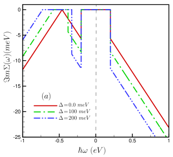
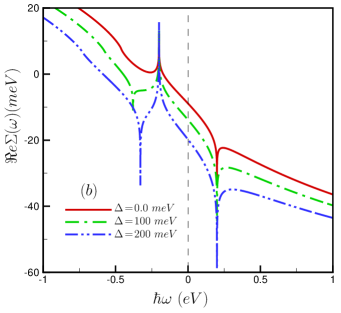
Figure 1: (Color online) Imaginary (a) and real (b) parts of the self-energy as a function of energy evaluated at Fermi energy for different gap values at the coupling constant $g=3.0$ and density $n=5.0\times 10^{12}$ cm^-2.

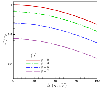
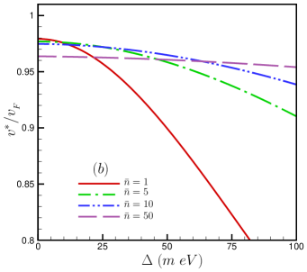
Figure 2: (Color online) Renormalized electron velocity for (a) the different values of coupling constants at $n=5.0\times 10^{12}$ cm^-2, (b) the different value of density (in units of $10^{12}$ cm^-2) at $g=3.0$.

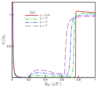
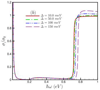
Figure 3: (Color online) Optical conductivity as a function of energy for (a) the different values of coupling constant at $\Delta=0.1~{}eV$ and (b) the different value of $\Delta$ at $g=3.0$. We consider $n=1\times 10^{13}~{}cm^{-2}$.

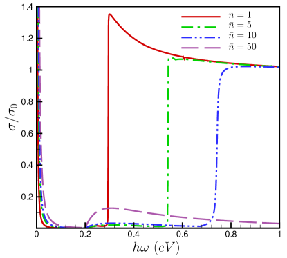
Figure 4: (Color online) Optical conductivity as a function of energy for different values of density ( in unites of $10^{12}$ cm^-2) at $g=3.0$ and $\Delta=0.1~{}eV$

References

- (1) O. Gunnarsson, Rev. Mod. Phys. 69 (1997) 575 and references therein.
- (2) K. S. Novoselov, A. K. Geim, S. V. Morozov, et.al., Science, 306 (2004) 666 .
- (3) Akin Akturk and Neil Goldman, Journal of Applied physics, 103 (2008) 053702 .
- (4) D. M. Basko and I. L. Aleiner, Phys. Rev. B 77 (2008) 041409 (R) .
- (5) Cheol-Hwang Park, Feliciaon Giustino, Marivin L. Cohen and Steven G. Louie, Nano Letters 8 (2008) 4229 .
- (6) T. Holstein, Ann. Phys. (N.Y.) 8, 325 (1959); 8 (1959) 343 .
- (7) S. Piscanec et al., Phys. Rev. Lett. 93 (2004) 185503 .
- (8) S. Piscanec et al., Phys. Rev. B 75 (2007) 035427 .
- (9) S. Pisana et al. Nature Mater. 6 (2007) 198 .
- (10) N. M. R. Peres, F. Guinea and A. H. Castro Neto, Phys. Rev. B 73(2006) 125411
- (11) N. M. R. Peres, and T. Stauber, Int. J. Mod. Phys. B, 16 (2008) 2529 .
- (12) T. Stauber, N. M. R. Peres, and A. K. Geim, Phys. Rev. B, 78 (2008) 085432 .
- (13) V. P. Gusynin, S. G. Sharapov and J. P. Carbotte, Phys. Rev. Lett. 96(2006) 256802 .
- (14) Z. Q. Li, et.al., Nat. Phys., 4(2008) 532 .
- (15) R. R. Nair et. al., Science, 320 (2008) 1308 .
- (16) T. Stauber, and N. M. R. Peres, J. Phys.: Condens. Matter 20 (2008) 055002.
- (17) M. Calandra and F. Mauri, Phys. Rev. B 76 (2007) 205411 .
- (18) W.-K. Tse and Das Sarma, Phys. Rev. Lett 99 (2007) 236802 .
- (19) N. M. R. Peres, T. Stauber and A. H. Castro Neto, EPL 84 (2008) 38002 .
- (20) T. Stauber, and N. M. R. Peres, Phys. Rev. B, 78(2008) 085418 .
- (21) S.Y. Zhou et. al., Nature Mater., 76 (2007) 770 .
- (22) K. S. Novoselov, et.al., nature 438(2005) 197 .
- (23) E. Cappelluti and L. Benfatto, Phys. Rev. B 79 (2009) 035419 .
- (24) A. Qaiumzadeh and R. Asgari, Phys. Rev. B 79 (2009) 075414 .
- (25) A. H. Castro Neto et al., Rev. Mod. Phys., 81 (2009) 109 .
- (26) Gerald D. Mahan, Many-Particle physics, (Plenum Peress, New York 1990) 2nd edition.
- (27) M. Jonson, and G. D. Mahan, Phys. Rev. B, 21 (1980) 4223 .
- (28) F. Dogan and F. Marsiglio, Phys. Rev. B 68 (2003) 165102 .
- (29) M. Polini et al., Phys. Rev. B 77 (2008) 081411(R) .
- (30) J. P. Carbotte, E. J. Nicol and S. G. Sharapov, arXiv:0908.2608 .