3D stellar atmospheres for stellar structure models and asteroseismology

Abstract

Convection is the most important physical process that determines the structure of the envelopes of cool stars. It influences the surface radiation flux and the shape of observed spectral line profiles and is responsible for both generating and damping solar-like oscillations, among others. 3D numerical simulations of stellar surface convection have developed into a powerful tool to model and analyse the physical mechanisms operating at the surface of cool stars. This review discusses the main principles of 3D stellar atmospheres used for such applications. The requirements from stellar structure and evolution theory to use them as boundary conditions are analysed as well as the capabilities of using helio- and asteroseismology to reduce modelling uncertainties and probing the consistency and accuracy of 3D stellar atmospheres as part of this process. Simulations for the solar surface made by different teams are compared and some issues concerning the uncertainties of this modelling approach are discussed.

1 Introduction – 3D Stellar Atmospheres

The inhomogeneous solar surface is characterised by large scale structures originating from the solar convection zone as well as from the complex solar magnetic field. Globally, the solar convection zone is dominated by an extreme density and temperature stratification with a contrast of $625,000:1$ and $350:1$, respectively, when comparing values for these quantities as found for the bottom of the solar convection zone with those found for its surface. The model data underlying these estimates are supported by helioseismology and solar surface observations (for further references related to these estimates see Kupka 2009). As a result the entire solar convection zone comprises 20 pressure scale heights spread over 30% of the solar radius. In spite of the slow solar rotation rate the timescales on which convection transports mass and heat through the entire zone are hence comparable to those of rotation. This does not hold for the surface layers of the Sun. With average velocities reaching 2 to 3 km s^-1 the granules and downflow regions observed at the solar surface change over timescales of a few minutes to less than half an hour, two orders of magnitudes faster than the timescale of rotation on these length scales. Similar holds for other types of stars with convection zones reaching the stellar surface provided that the surface gravity is high enough such that the pressure scale height at optical depths of order unity is just a small fraction of the stellar radius.

These physical relations are the main background for the “box-in-a-star” approach to 3D stellar atmospheres. In this case, a small volume of the entire convection zone is considered for which the conservation law equations for the densities of mass, momentum, and energy, have to be solved. The hydrodynamical equations are coupled to the equation for radiative transfer, which have to be solved as well, since at the surface of a star the diffusion approximation is no longer valid. Realistic hydrodynamical simulations of such a system require a tabulated equation of state and tabulated opacities computed for the chemical composition assumed for the object to be studied. The simulations performed for this setting describe the evolution of such a sample volume of the stellar atmosphere (and upper envelope) in space and time, as represented on a grid extending over the entire simulation box and computed for a finite number of time steps. The capabilities of this approach and its successful recovery of observational data such as surface intensity images in the visual or detailed spectral line profiles have been discussed in many research papers and conference reviews (cf. Stein & Nordlund 1998 as well as examples and references in Asplund 2007, Steffen 2007, Kupka 2009, and the extensive review of Nordlund, Stein, & Asplund 2009).

In the following we provide a short review on how 3D stellar atmospheres can be used for the modelling of stellar structure and for helio- and asteroseismology. We discuss requirements on model stellar atmospheres posed by these branches of stellar physics and some applications to illustrate the demands on the 3D models. More recently, 3D stellar atmospheres have been used to compute physical quantities difficult to access by means of direct observations or even seismology, such as turbulent pressure or skewness of vertical velocities below the visible solar or stellar surface. We provide some first results from a comparison of different 3D stellar atmospheres used to compute statistically averaged quantities required in stellar structure modelling and seismology. We also discuss some issues related to the resolution of 3D models and conclude this paper with a summary.

2 Stellar Modelling

A solar structure model or a stellar evolution track depends on a variety of hydrodynamical processes including convection. Since the associated hydrodynamical timescales are many orders of magnitudes shorter than the thermal and nuclear ones during most phases of stellar evolution, 3D hydrodynamical simulations of solar or stellar evolution are computationally too demanding. This restriction holds even for simulations of solar convection on just the hydrodynamical timescales because of extreme stratification (20 pressure scale heights from the top to the bottom of the zone).

From a stellar structure modelling point of view convection models are required, among others, to compute stellar radii of stars which have convective envelopes. For this purpose tables of the mixing length parameter and turbulent pressure obtained from hydrodynamical simulations of the surface convection zones would in principle be sufficient (see Ludwig, Freytag, & Steffen 1998, Trampedach et al. 1999, and more recent work from the same authors for some examples). But for stellar evolution modelling such tables are inadequate. In particular, these tables would not describe the nature of convection in the stellar interior, where we need to compute the amount overshooting of convective zones into radiative ones, the precise convective efficiency in those transition regions, and other phenomena which occur in stellar interiors such as semi-convection and further varieties of double-diffusive convection. The currently used analytical, semi-empirical formulae for the description of these physical processes suffer from inconsistencies (cf. the discussions in Canuto & Mazzitelli 1991; Canuto 1993; Charbonnel & Zahn 2007). Hence, the development of improved calibration methods is highly rewarding as are more refined simulations, which would be suitable for deducing more versatile convection models.

Classical procedures for the computation of stellar models with convective envelopes such as calibrating the mixing length have some severe limitations. Among others, they are based on integral quantities (radius, luminosity, etc.). Unless secondary calibration methods are used (which in turn require stellar models), these quantities are known only for rather few, nearby stars with sufficient accuracy. In the end, such methods are an ambiguous probe of convection models.

Methods based on detailed photospheric properties alone (such as comparing observed with computed spectral line profiles) require quantities such as the mean temperature to be properly modelled as a function of depth. They hence provide some extra information to reduce ambiguities in calibrations and models tests, but they have only limited implications on how convection is modelled in the stellar interior and can still remain inconclusive for photospheric convection modelling (cf. Montalbán et al. 2004 and Heiter et al. 2002, for example).

3 Helioseismology and Asteroseismology

Helio- and asteroseismology have opened a new window to look inside stars. They allow a much more thorough understanding of the mean structure and hydrodynamical properties of stellar interiors due to convection and rotation. Traditional “seismological tests” of convection models are based on frequency information obtained from helioseismological or asteroseismological observations. But in spite of the constraints they provide on measurements of the depth of the solar convection zone, on the extent of deviations from a radiative temperature gradient in the layers right underneath the solar convection zone (overshooting), or on the chemical composition, these methods are still limited by ambiguities. One of the reasons is that the acoustic size of a resonant cavity can be the same for different model structures within the frequency domain which is accessible to measurements with sufficient accuracy. This is the physical background for two contradicting explanations suggested for the differences between observed solar p-mode frequencies and predicted ones based on standard solar models (Basu & Antia 1995 found that a much steeper superadiabatic temperature gradient as obtained with the convection model by Canuto & Mazzitelli 1991, 1992 reduces the discrepancy between observations and computations, while a similar reduction was found when using averaged model structures from 3D hydrodynamical simulations of the surface layers by Rosenthal et al. 1999, who pointed out the role of turbulent pressure and differences in the model structure originating from the 3D, inhomogeneous radiative transfer — see also Canuto & Christensen-Dalsgaard 1998 for further discussion).

Observational data on amplitude and time dependence (mode linewidth and lifetime) of the p-modes, i.e. the study of p-mode excitation and p-mode damping, provides the extra information necessary to remove such ambiguities. Mode excitation occurs due to shear stresses and entropy fluctuations. Based on earlier work by Goldreich & Keeley (1977) and Balmforth (1992), different semi-analytical models have been developed (see Houdek et al. 1999; Samadi & Goupil 2001; Houdek 2002; Chaplin et al. 2005). Through predictions of velocity and convective flux these models link observations with quantities required to construct stellar models. Models or numerical simulations are used to compute eigenfunctions and associated eigenfrequencies, the mean structure (density, entropy, …), spatial and temporal correlations of velocity and entropy as a function of length scale, the filling factor (fraction of horizontal area covered by upflows), and the ratio of vertical to horizontal root mean square velocities.

Observations (with some modelling) provide quantities such as mode mass, the height above the photosphere where the modes are measured, the mode line width at half maximum, and the mean square of the mode surface velocity. Samadi et al. (2006) have used standard solar structure models to compute the model dependent input data for the approach of Samadi & Goupil (2001) required to calculate p-mode excitation rates. They investigated the influence of non-grey atmospheres in comparison with the grey diffusion approximation and compared a standard mixing length model of convection with the model of Canuto, Goldman, & Mazzitelli (1996). The standard model (grey, mixing length treatment of convection) underestimates excitation rates by up to an order of magnitude. Convection treatment was found to be more important for the excitation rate calculation than line blanketing (non-grey atmospheres), but eventually also the convection model by Canuto, Goldman, & Mazzitelli (1996) combined with a non-grey atmosphere, as in Heiter et al. (2002), was found to yield a model structure that still underestimates p-mode excitation rates by up to a factor of 3.

By comparison, numerical simulations were found to reproduce observed excitation rates under the assumption of a non-Gaussian temporal correlation (Samadi et al., 2003). A new, semi-analytical model to compute p-mode excitation rates was presented by Belkacem et al. (2006a). It is based on the model of Gryanik & Hartmann (2002) and Gryanik et al. (2005) for computing third and fourth order correlation functions in flows dominated by turbulent convection. This model accounts for asymmetry between up- and downflows (skewness of velocity and temperature). Due to mass conservation a flow with broad upflows (granules !) has higher velocities in its downflows and since the input power for p-modes depends quadratically on the velocity, the total input power increases in this case. Belkacem et al. (2006b) have shown that this model together with the assumption of a Lorentzian distribution function taken for the temporal correlations predicts solar p-mode excitation rates in agreement with observations. We note at this point that some of the input for their model had to be taken from numerical simulations (for instance, the horizontal area fraction covered by upflow regions).

The applicability of their new approach to stars other than the Sun was shown by Samadi et al. (2008) by computing mode excitation rates for $\alpha$ Cen A and comparing them with observational predictions. The model predictions were found in agreement with the data, but it was also pointed out that a higher accuracy of asteroseismological measurements is still needed to provide sufficiently tight constraints for the models, which is now possible with the results from the CoRoT mission (Appourchaux et al. 2008; Michel et al. 2008) and soon by the Kepler mission. This demonstrates that helio- and asteroseismology have the capability to falsify models and simulations where classical methods remain ambiguous.

4 Comparing Simulations, Resolution Issues

How well do the currently available numerical simulations of surface convection agree about the mean structure of the uppermost layers of stars and on the correlation functions required to interpret data from helio- and asteroseismology? To find an answer one should consider, among others, the following questions: to what extent is the flow influenced by the boundary conditions? How large is the influence of the domain size? How important is non-grey radiative transfer for the structure of the superadiabatic layer developed by convection zones that reach the stellar surface? Do different numerical methods and viscosity models change the large scale (coherently structured) part of the flow?

In the following we discuss some first results of a comparison of solar surface convection simulations performed with four different simulation codes. Each of these 3D simulations is set up for the “box-in-a-star” scenario with a rectangular box covering only a small fraction of the stellar surface layers, with a constant surface gravity, and with periodic boundaries along the horizontal directions. Results for the CO⁵BOLD (Freytag, Steffen, & Dorch, 2002) have kindly been provided by M. Steffen. This code uses a Roe-scheme for advection (i.e. a non-linear numerical viscosity) combined with a subgrid-scale viscosity (Smagorinsky, 1963). For the two simulations shown the vertical boundaries are open and the chemical composition assumed is that one of Grevesse & Sauval (1998). The high resolution case shown assumes non-grey radiative transfer (with 5 opacity bins), a box volume of $11.2^{2}\times 3.1$ Mm³, a grid of $400^{2}*165$ points, a constant horizontal grid size of $28$ km and a variable vertical one of $12\dots 28$ km. The deep simulation assumes grey radiative transfer, a box volume of $11.2^{2}\times 5.2$ Mm³, a grid of $200^{2}\times 250$ points, a constant horizontal grid size of $56$ km and a fixed vertical one of $21$ km.

Two further simulations have kindly been provided by F.J. Robinson and are based on the simulation code presented in Kim & Chan (1998) and Robinson et al. (2003) (named CKS code in the figures). Its numerical scheme uses plain second order finite differences with a subgrid-scale viscosity (Smagorinsky, 1963) where the coefficients are boosted near shock fronts. Both sets have closed vertical boundaries and grey radiative transfer is assumed, with a 3D Eddington approximation. The simulation with smaller domain size (“case D” from Robinson et al. 2003) assumes a chemical composition as in Grevesse & Noels (1993) and has a box volume of $2.9^{2}\times 3$ Mm³, a grid size of $58^{2}\times 170$ points, a constant horizontal grid size of $50$ km and a fixed vertical one of $17.6$ km. The “2008” simulation assumes the chemical composition of Grevesse & Sauval (1998) and has a box volume of $5.4^{2}\times 3.6$ Mm³, a grid of $117^{2}\times 190$ points, a constant horizontal grid size of $46$ km and a fixed vertical one of $19$ km.

Another simulation, performed with the code by Stein & Nordlund (1998), has kindly been provided by R. Samadi and K. Belkacem (it is essentially the one used by Belkacem et al. 2006a). The advection scheme of this code is stabilized with hyperviscosity and an extra viscosity near shock fronts. Open vertical boundary conditions are assumed and for this simulation the chemical composition is similar to that one published by Grevesse & Sauval (1998). A non-grey radiative transfer (with 4 bins) is assumed as well as a box volume of $6^{2}\times 3$ Mm³, a grid of $150^{3}$ points, a constant horizontal grid size of $40$ km and a variable vertical grid with an average spacing of $20$ km.

Finally, we present results from a new simulation performed with the ANTARES code (Muthsam et al., 2007, 2009). Due to its high order advection scheme based on essentially non-oscillatory methods, i.e. a non-linear numerical viscosity, physical viscosity sources (radiative and molecular ones) are sufficient to stabilize the code for the photospheric layers contained in the simulation. For the stellar interior their contributions are negligible and the numerical scheme is stable without adding subgrid-scale or artificial diffusivities. For this simulation the chemical composition presented in Grevesse & Noels (1993) is used together with a box volume of $6^{2}\times 3$ Mm³, a grid of $150^{2}\times 190$ points, a constant horizontal grid size of $40$ km and a constant vertical grid spacing of $16$ km, and grey radiative transfer is assumed.

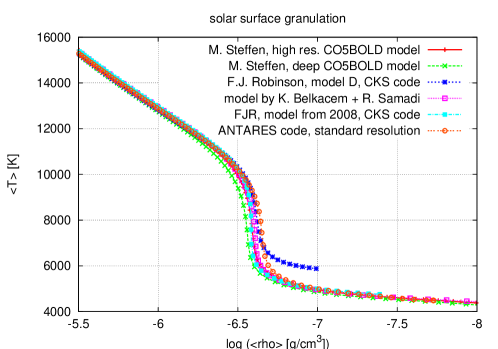
Figure 1: Horizontally averaged mean temperature $T$ as a function of the logarithm of the horizontally averaged mean density $\rho$ for the six simulation sets. The region shown includes the uppermost layers of the solar interior, the superadiabatic peak, and the lower photosphere.

In Fig. 1 we compare the horizontally averaged mean temperature $T$, plotted as a function of the logarithm of the horizontally averaged mean density $\rho$, for all six simulation sets. The averaging was performed for each horizontal layer and each point in time followed by a time average. Since there is no inversion of the mean density as a function of depth in any of the simulations, there is a unique mapping of the mean density to depth and radius for each simulation. In the interior all simulations agree very well with each other. Near the superadiabatic peak the maximum spread in mean density for a given mean temperature is $\pm 15\%$ and is due to different metallicities, different resolution, and different treatment of radiative transfer schemes being used. For the lower photosphere all but one of the simulations agree again quite well (the exception is the “case D” model which does not extend far enough into the photosphere to produce realistic temperatures in that region). For the mid and upper photosphere, which are not shown here, the simulations with grey radiative transfer yield higher average temperatures, although the detailed behaviour for the outermost layers also depends on the exact implementation of the boundary conditions.

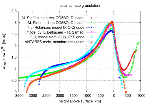
Figure 2: Root mean square values of horizontally averaged vertical velocity fluctuations of all six simulations.

In Fig. 2 we compare the root mean square values of the horizontally averaged vertical velocity fluctuations of all six simulations. Despite the simulations with closed boundary conditions have $w_{\rm rms}$ values which tend towards zero near the top, they behave very similarly to the simulations with open vertical boundaries for the layers at the solar surface up to the highest velocities, which are found around the superadiabatic peak. Only the shallow “model D” computed with the CKS code and the lower resolution, deep model computed with the CO⁵BOLD code predict slightly lower maximum values. Further inside, both simulations with the CKS code predict higher values for $w_{\rm rms}$, which drops rapidly near the closed bottom. In turn, the averages from the ANTARES code are very similar to those computed by K. Belkacem and R. Samadi with the code by Stein & Nordlund (1998) from the solar surface close to the bottom of the simulation volume. Note the different behaviour of the simulation codes using open vertical boundaries near the top of the simulation domain (increasing vs. constant $w_{\rm rms}$).

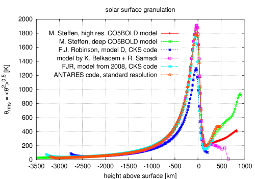
Figure 3: Root mean square values of the horizontally averaged temperature fluctuations of all six simulations.

In Fig. 3 we compare the root mean square values of the horizontally averaged temperature fluctuations of all six simulations. Differences in the mid and upper photosphere originate from the non-grey radiative transfer assumed in some of the simulations. Except for the most shallow model, which has lower peak values, the root mean square fluctuations agree well among all of the simulations throughout most of the convection zone. Simulations with non-grey radiative transfer have larger peak values by only a few percent. Simulations with closed lower vertical boundary can be distinguished by an increase of temperature fluctuations close to the bottom boundary layer.

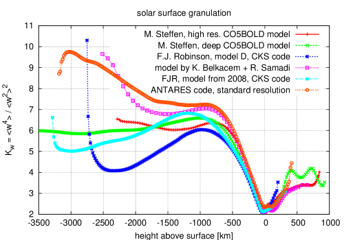
Figure 4: Kurtosis $K_{w}$ of horizontally averaged vertical velocity fluctuations for all six simulations.

In Fig. 4 we compare the kurtosis $K_{w}$ of the horizontally averaged vertical velocity fluctuations for all six simulations. We note that again all simulations agree for the layers from the bottom of the photosphere till below the superadiabatic peak. However, further below the differences become large despite long-term averages performed over about 4 to 12 hours of solar time (about 15 to 50 convective turnover times) have been used. In particular, simulations with open vertical boundaries do not (!) agree more closely among each other when compared to simulations with closed vertical boundaries. This is an important caveat to remember when using 3D stellar atmospheres to compute data for helio- and asteroseismology. Clearly, the higher order correlations are much more sensitive to the details of the implementation of the boundary conditions than the variables representing only the mean structure of the simulation domains.

Since the simulations compared above have the same resolution within a factor of two, one might argue how they depend on numerical methods used and on resolution in general. None of the simulations compared above can be expected to resolve turbulence created by shear between up- and downflows, since in 3D one expects a horizontal and vertical resolution of less than 5 km to be required for that (Kupka, 2009). Questions related to resolution include whether the spectral line profiles remain unaffected by turbulence generated through shear underneath the visible surface, what are the contributions of turbulence to Reynolds stresses and entropy for p-mode driving, or whether a better resolved radiative cooling at the stellar surface does change the flow properties. Resolution effects in 3D stellar atmosphere for grid spacings similar to the simulations discussed above have been discussed by Stein & Nordlund (1998) and Robinson et al. (2003), among others. Recently, Muthsam et al. (2009) have demonstrated that for this resolution the diffusion of the advection scheme in the simulation clearly has an influence on the small scale structures at the visible surface. However, horizontal resolutions of 10 km with the least dissipative numerical scheme are necessary to finally reveal the highly turbulent nature of downdrafts underneath the solar surface rather than just noticing indications for their turbulent behaviour. At the transition between laminar and turbulent flow the effective resolution of a numerical scheme is crucial, since only for even higher resolution (i.e. in the turbulent regime) such numerical details can be expected to no longer matter. The influence of shear driven turbulence on observable quantities has yet to be investigated.

5 Summary

Hydrodynamical simulations have developed into a tool for the computation of realistic 3D stellar atmospheres of cool stars. Particularly for stars at or close to the main sequence they have successfully passed observational tests based on spectroscopy and traditional calibration methods for convection models, but also tests based on helioseismology, which can distinguish much more sensitively between different physical models of the outer envelope of the Sun. Asteroseismology is now gradually gaining the same capability. Current numerical simulations of solar surface convection are robust in their predictions of the mean solar surface structure (different boundary conditions, radiative transfer treatment, resolution) and pass observational tests which require moderate spatial resolution. However, a comparison of higher order correlation functions for velocity (and temperature) demonstrates that these quantities are sensitive to the implementation of boundary conditions. Interestingly, they could be tested by means of helio- and asteroseismology. Refined advection numerics and high spatial resolution show how turbulence is generated in downflows shrouded by the surface layers (cf. also Stein & Nordlund 2000 for a first study of this question).

Thus, 3D stellar atmospheres provide stellar evolution modelling with a tool to calibrate convection models and improve stellar evolution calculations. Both spectroscopy and asteroseismology will continue to help in defining the region of applicability of numerical simulations of stellar convection. At the same time, questions related to mixing due to convection zones and their behaviour deep inside the stars remain open. A convection model taking these processes into account is still in demand.