Mapping the Asymmetric Thick Disk I. A Search for Triaxiality

Abstract

A significant asymmetry in the distribution of faint blue stars in the inner Galaxy, Quadrant 1 (l $=20\arcdeg-45\arcdeg$) compared to Quadrant 4 was first reported by Larsen & Humphreys (1996). Parker et al (2003, 2004) greatly expanded the survey to determine its spatial extent and shape and the kinematics of the affected stars. This excess in the star counts was subsequently confirmed by Jurić et al. (2008) using SDSS data. Possible explanations for the asymmetry include a merger remnant, a triaxial Thick Disk, and a possible interaction with the bar in the Disk. In this paper we describe our program of wide field photometry to map the asymmetry to fainter magnitudes and therefore larger distances. To search for the signature of triaxiality, we extended our survey to higher Galactic longitudes. We find no evidence for an excess of faint blue stars at l $\geq 55\arcdeg$ including the faintest magnitude interval. The asymmetry and star count excess in Quadrant 1 is thus not due to a triaxial Thick Disk.

1 Introduction: The Asymmetric Thick Disk

Studies of both stars and gas are revealing significant structure and asymmetries in their motions and spatial distributions including the bar of stars and gas in the Galactic bulge (Blitz & Spergel 1991, Stanek et al. 1994), the evidence from infrared surveys for a larger stellar bar in the inner disk (Weinberg 1992, Lopez-Corredoira et al. 1997, Benjamin et al. 2005), the discovery of the Sagittarius dwarf (Ibata et al., 1994; Ibata & Gilmore, 1995), and a significant asymmetry of unknown origin in the distribution of faint blue stars in Quadrant 1 (Q1) of the inner Galaxy (Larsen & Humphreys, 1996). Each of these observations provides a significant clue to the history of the Milky Way. When combined with the growing evidence for Galactic mergers in addition to the Sagittarius dwarf, i.e. the Monoceros stream (Newberg et al. 2002, Ibata et al. 2003), the Canis Major merger remnant (Martin et al. 2004), the Virgo stream (Vivas et al. 2001, Martínez-Delgado et al. 2005), we now realize that the structure and evolution of our Galaxy have been significantly altered by mergers with other systems. Indeed the population of the Galactic Halo and possibly the Thick Disk as well, may be dominated by mergers with smaller systems.

The asymmetry in Q1, $l=20\arcdeg-45\arcdeg$, first recognized by Larsen & Humphreys (1996) was based on a comparison with complementary fields in the fourth Quadrant (Q4) using star counts from the Minnesota Automated Plate Scanner Catalog of the POSS I (Cabanela et al., 2003). To map the extent and shape of the asymmetric distribution and further identify the contributing stellar population, Parker et al. (2003) extended the search to 40 contiguous fields from the digitized POSS I on each side of the Sun-Center line plus the same number of fields below the plane in Q1. They examined the star count ratios for paired fields in three color ranges: blue, intermediate and red. Over 6 million stars were used in the star count analysis covering almost 2000 square degrees on the sky. They found a 25% excess in the number of probable Thick Disk stars in Q1, $l\approx 20$ to $60\arcdeg$ and $20\arcdeg$ to $40\arcdeg$ above and below the plane compared to the complementary fields ($l\approx 340$ to $300\arcdeg$) in Q4. While the region of the asymmetry is somewhat irregular in shape, it is also fairly uniform and covers several hundred square degrees. It is therefore a major substructure in the Galaxy due to more than small scale clumpiness. Assuming that these are primarily main sequence thick disk stars, with a typical magnitude completeness limit of $V\approx 18$ mag, they are 1 - 2 kpc from the Sun and about 0.5 to 1.5 kpc above (and below) the plane.

Parker et al. (2004) also found an associated kinematic signature. Using velocities from spectra for more than 700 stars, they not only found an asymmetric distribution in the v_LSR velocities, but the Thick Disk stars in Q1 have a much slower effective rotation rate $\omega$ compared to the corresponding Q4 stars. A solution for the radial and tangential components of the v_LSR velocities reveals a significant lag of 80 to 90 km s^-1 in the direction of Galactic rotation for the Thick Disk stars in Q1.

Three possible explanations for the asymmetry are the fossil remnant of a merger, a triaxial Thick Disk or inner Halo, and interaction of the Thick Disk/inner Halo stars with the bar in the Disk. Given the lack of any spatial overlap with the path of the Sagittarius dwarf through the Halo (Ibata et al., 2003), and the predicted path of the Canis Major dwarf (Martin et al., 2004), its association with either feature is unlikely. Furthermore its spatial extent and apparent symmetry relative to the plane also do not automatically support a merger interpretation. Our line of sight to the asymmetry is interestingly in the same direction as the stellar bar in the Disk (Weinberg, 1992; Benjamin et al., 2005), and the near end of the Galactic bar (Lopez-Corredoira et al., 1997; Hammersley et al., 2000), but the Disk bar is approximately 5 kpc from the Sun in this direction. Thus the stars showing the excess are between the Sun and the bar, not directly above it. However the maximum extent of the star count excess along our line of sight is not known.

Recently Larsen et al. (2008) showed the stellar density distribution from the MAPS scans for the Parker et al. (2003) fields in Q1 and Q4 above the plane, demonstrating that the excess was in Q1 and was not due to a ring above the plane (Jurić et al., 2008). Larsen et al named the asymmetry feature the Hercules Thick Disk Cloud in recognition of the direction on the sky where the star count excess is maximum. Thus, interpretation of the Hercules Thick Disk Cloud is not clear-cut. While it might well be a fossil merger remnant, the star count excess is also consistent with a triaxial Thick Disk or inner Halo as well as a gravitational interaction with the stellar bar especially given the corresponding asymmetry in the kinematics. The distinction between a triaxial Thick Disk and interaction with a Disk bar may be difficult to discern. Indeed, it is unclear which may have formed first, and one or both may be the result of mergers.

The release of the SDSS Data Release 5 (DR5) photometry in the direction of the observed asymmetry in Q1 led to the discovery of a feature at much fainter magnitudes, the distant Hercules-Aquila cloud (Belokurov et al., 2007) and also confirmed the nearer star count excess in the inner Galaxy (Jurić et al., 2008). The SDSS survey however is not well designed for a comprehensive survey of the Thick Disk inside the Solar orbit. It extends below $b=30\arcdeg$ in only a few directions in Q1 and has only limited coverage in Q4. It does not have the leverage in Galactic longitude needed to discriminate among the possible causes of the Hercules Thick Disk Cloud.

To further explore the possible origin of the observed spatial and kinematic asymmetry, we have obtained multicolor CCD images to extend the star counts to fainter magnitudes to map the spatial extent of the asymmetry along the line of sight as a function of Galactic longitude and latitude. For example, if the Thick Disk is triaxial we would expect to observe the star count excess out to greater longitudes, but the star count excess described by Parker et al. (2003) appears to terminate near l $\sim$ 55$\arcdeg$. However, if it is triaxial in Q1 with its major axis above the bar, the stars would be further away at the higher longitudes. By extending the star counts to fainter magnitudes, corresponding to greater distances, we can search for the asymmetry at higher longitudes, from l of 50$\arcdeg$ to 75$\arcdeg$.

In this first paper we describe our observing program and present results on a search for triaxiality of the inner Halo and Thick Disk. Our second paper will discuss the star counts across the full range of longitudes in Q1 and Q4 containing the asymmetry feature and a third paper in the series will analyze the kinematics of the associated stars. In the next section we describe the CCD observing program and data reduction. Determination of the star count ratios and their errors for the fields at the higher longitudes are discussed in §3. Our results do not support a triaxial interpretation of the asymmetry feature and are summarized in §4.

2 Observations and Data Reduction

To map the asymmetry feature both above and below the Galactic plane we identified 67 fields ranging in longitude from l = 20$\arcdeg$ to 75$\arcdeg$, and l = 340$\arcdeg$ to 285$\arcdeg$ and latitude b = $\pm$20$\arcdeg$ to $\pm$45$\arcdeg$. The total sky coverage of the program is 47.5 square degrees. The distribution of our program fields on the sky is shown in Figure 1 and the information for each field is given in Table 1 with their Galactic and equatorial centers, instrument, field size and date of observation . In this paper we will be discussing a subset of the fields relevant to the triaxiality question. These fields are circled on Figure 1 and are listed in Table 6. Our program required observations in both hemispheres.

2.1 Northern Hemisphere - Steward Observatory Bok 2.3 Meter

We used the Steward Observatory 2.3 meter Bok telescope with the 1 square degree 90Prime camera in 2006 May, 2007 September and 2008 May. This mosaic camera has 4 blue sensitive 4096x2096 CCDs. Counting cosmetic defects and the plate scale of 0.45″ per pixel we had an effective field of view of approximately 1.02 square degrees. The CCDs are arranged in a square with intra-CCD gaps of about 10 arcminutes. We used a Johnson U,B,V + Cousins-Kron R filter set for the observations. This field of view was ideal for the project as it allowed each of the project fields to be observed in a single pointing.

Program fields were observed twice in each filter with exposure times of 600 seconds in U, 480 seconds in B, and 90 seconds each in V and R. Exposure times were chosen to reach a limiting magnitude of 20th in U and 22nd in B, V and R. These exposures were of sufficient length to require autoguiding. The filters were not parfocal but focus was digital and corrections were easily applied.

We reduced the data with the IRAF MSCRED mosaic image reduction package (Valdes, 1998). The data were corrected for cross talk, bias, and dark current. Flatfielding was done using night-sky flats from program fields supplemented by a series of random sky exposure with equivalent exposure times. CCD defects, bad pixels and satellite trails were removed.

Astrometry was done with Larsen’s MOSAF (Mosaic Astrometry Finder) program written for the Spacewatch 0.9 meter telescope (Larsen et al., 2007) which uses a 13 term polynomial for a plate model, the CFITSIO library (Pence, 1999) and WCSLib from WCSTools (Mink, 1999). The astrometric reference catalog was USNO-B1.0 (Monet et al., 2003), and the residuals were approximately 0.3″  in all frames.

Photometric reductions used both Landolt Standards (Landolt, 1992) and a secondary set of faint standards from Osmer et al. (1998), and followed the method of Hardie (1964). The formal zero point errors were approximately 0.03 magnitudes per filter with the photometric RMS of 0.05 magnitudes per band. An example of the mean atmospheric extinction and color terms can be found in Table 2; seeing varied from 1.0″  to 2.8″  during the 2006 May observations.

2.2 Southern Hemisphere - CTIO SMARTS 1.0 Meter

Fields which could not be reached with the Bok 2.3 meter telescope were observed using the Y4KCam at the 1.0 meter SMARTS consortium telescope at CTIO in 2006 April and 2008 October. This camera is a 4096x4096 pixel single CCD with a plate scale of 0.289” per pixel and a field of view of about 0.108 square degrees. Consequently, 9 subfields were observed to yield an effective area of $\approx$ 0.95 square degrees with overlap. The Johnson U,B,V + Cousins-Kron R filter set was used for these observations.

Program fields were observed once in each filter. During 2006 April, the exposure times were 300s in U, 150s in B, and 60s in the V and R bands. This was sufficient to reach 19th magnitude in B. V and R and 18th magnitude in U. In 2008 October, the exposure times were increased to 400s in U, 485s in B, 160s in V and 190s in R to reach fainter magnitudes. These exposures were of sufficient length to require autoguiding. The filters were not parfocal but could be compensated by a focus reduction.

Our initial processing of the frames was based on the IRAF scripts for the Y4KCam provided by Massey. Flat fielding used both dome and twilight flats. Astrometry was done using WCSTools and the USNO-B1.0 catalog with results refined and checked against MOSAF. Seeing was moderate for the 2006 April observations, with FWHM from 1.5″  to 3.0″ .

Photometric reductions used both Landolt Standards (Landolt, 1992) and a secondary set of faint standards from Osmer et al. (1998). Photometric magnitudes were then determined using the same method as the 90Prime data to assure consistency. Examples of the mean atmospheric extinction and color terms are in Table 3.

2.3 Catalog Creation

Source detection, image parametrization and catalog creation used Source Extractor (Bertin & Arnouts, 1996). After several tests to verify that we were detecting objects close to the image limits, the default size for the Gaussian convolution mask was used and magnitudes were determined using the MAG_AUTO feature which uses an adaptive aperture photometry routine. Aperture photometry was performed on the detected objects. Since most are stars, they were not subject to the same faint-end systematics as galaxies (Bernstein et al., 2002). We also discarded all objects detected within 4″  of the edge of the frame as potentially truncated.

A custom pipeline was written to apply the WCS astrometry solution and photometric calibration to each object in the catalogs for each field. We then used the WCS positions to match the objects observed in the different filters. To be included in the final catalog, each object had to be measured in at least two filters to provide color information. Problems with the star-galaxy classifier in Source Extractor are discussed in the next section.

The final catalogs with magnitudes, positions, colors and object classifications will be available on-line with the second paper.

2.4 Star Galaxy Separation

The neural network classifier in Source Extractor does not work on images with pixel scales similar to those in our data. We therefore developed our own simple classifier, called JAL, based on image parameters from Source Extractor sensitive to the differences between point sources and extended objects. We conducted a series of tests of the various image parameters to find three that were suitable for a simple parameter space cut which could be applied to each image. The following three parameter space comparisons were adopted:

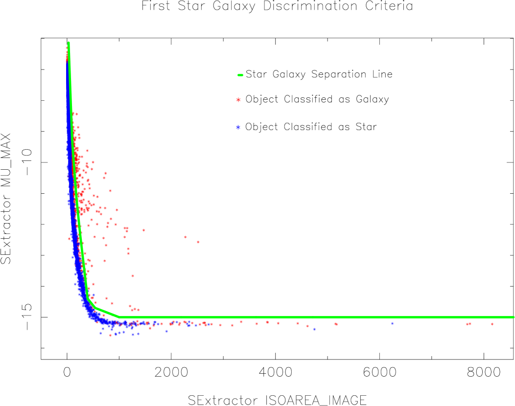
Figure 2: Star/galaxy separation with MU_MAX vs. ISOIMAGE_AREA. The stellar locus is well defined. The plot represents all points on amplifier ”A” of 90Prime during a 120 second R band exposure on the night of May 26, 2006. The discrimination line is plotted in green. Objects which are classified as a galaxy when all three discriminators are applied are plotted in red while objects which remain on the stellar locus are plotted in blue.

1. MU_MAX vs. ISOAREA_IMAGE captures the tendency of extended objects to have a surface brightness much lower than a star at the same isophotal diameter. A sample parameter space is shown in Figure 2, with the discriminator curve separating stars from galaxies.

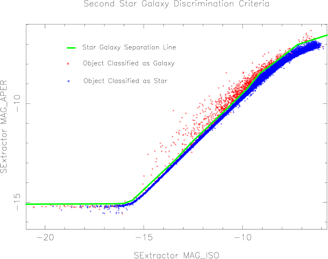
Figure 3: Star/galaxy separation with MAG_ISO versus MAG_APER. The plot represents all points on amplifier ”A” of 90Prime during a 120 second R band exposure on the night of May 26, 2006. The discrimination line is plotted in green. Objects which are classified as a galaxy when all three discriminators are applied are plotted in red while objects which remain on the stellar locus are plotted in blue.

2. MAG_ISO vs. MAG_APER isolates the tendency of extended objects to have a substantial fraction of its light outside of the core of the PSF, generating an isophotal magnitude larger than the aperture magnitude. An example of this parameter space is shown in Figure 3, with the discriminator curve separating stars from galaxies.

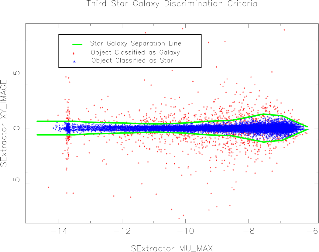
Figure 4: Star/galaxy with XY_IMAGE versus MU_MAX. The plot represents all points on amplifier ”A” of 90Prime during a 120 second R band exposure on the night of May 26, 2006. The discrimination line is plotted in green. Objects which are classified as a galaxy when all three discriminators are applied are plotted in red while objects which remain on the stellar locus are plotted in blue. The spike in the XY_IMAGE direction which occurs at MU_MAX $\sim$ 13.7 is due to charge bleed for the brightest objects. Since these objects are already saturated they are not contaminating our star count samples.

3. XY_IMAGE vs. MU_MAX shows how an extended object tends to have a moment in the intensity distribution much different than a star at the same peak surface brightness. The sample parameter space for these parameters is shown in Figure 4, with the discriminator curve separating stars from galaxies. This is the weakest of the three criteria and is therefore given one-half the weight of the other tests.

We used these three discriminators in a simple Perl/Pgplot routine which allowed the user to interactively define a curve separating stars (scored as 0) from galaxies (scored as 1). The net classification for a given image was a weighted score of 0 to 1 averaged from the three tests. During the final catalog matching an averaged net score was then computed from the V and R bands only. We conservatively considered an object with a average score greater than 0.3 to be a galaxy.

We developed this method by comparison with other classifiers. Training and fine-tuning the parameter spaces was done using stars and galaxies classified with FOCAS in the Osmer and Hall standard fields observed each night. As a final test, we chose a 90Prime field (H055+42) in the MAPS Catalog of the POSS I with object classification using a neural network (Odewahn et al., 1992, 1993) which was also observed and classified by SDSS. The results of our comparison as a function of magnitude are in Tables 4 and  5 for the MAPS and SDSS, respectively. For $V>16$, our classifier agreed with the APS classification 89% of the time or better and with SDSS 95% of the time or better. The lower agreement with the MAPS can be attributed to blended images on the MAPS scans which were classified as non-stellar or galaxies. The poor agreement with both APS and SDSS for $V<16$ is easily explained by the onset of saturation in the 90Prime images for our exposure times.

2.5 Comparison with SDSS

Six of our program fields overlap SDSS. Figure 5 shows a photometry comparison between objects classified as stars by both SDSS and our classifier for the program field H055+42. The SDSS stars have been transformed to the standard V band (Rodgers et al., 2006). For this comparison we find a zero point difference of 0.02 magnitudes. For $V\leq 20.0$ the RMS difference between SDSS magnitudes and ours is 0.04 magnitudes, for $20.0<V\leq 21.5$ the deviation is 0.09 magnitude and for $V>21.5$ it is 0.31 magnitude. Our data is thus well-suited for our star count analysis down to $V\sim 21$.

2.6 Extinction Corrections

Our magnitudes and colors were corrected for interstellar extinction using the maps from Schlegel et al. (1998) and the standard interstellar extinction law (Cardelli et al., 1989). Each star was corrected based on its coordinates using the interpolation routines provided. This approach assumes that the extinction comes from relatively near the Sun and is applied as a constant correction. Because our fields are intermediate to high galactic latitudes, extinction is relatively low. All but two fields have an average $E(B-V)$ of less than 0.08. One high extinction field (H300-20) has an average $E(B-V)$ of 0.36. The extinction-corrected color-magnitude diagram resembled the other fields with the placement of the blue ridge at the expected $B-V$ color. Therefore extinction anomalies do not play a role in our evaluation of the star counts.

2.7 Completeness Estimates

The classical estimate of the completeness limit is determined from a plot of the log of the cumulative star counts vs. magnitude and determining the magnitude at which it deviates from the expected straight power law. For galactic structure work at the magnitudes we are considering however, this classical method does not work well because the density of Thick Disk stars changes with distance above the plane of the Galaxy. At fainter magnitudes there are simply fewer stars to be found at larger distances which can look like incompleteness.

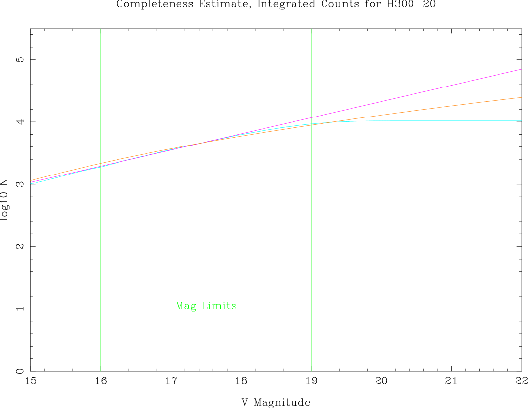
Figure 6: Integrated counts for field H300-20 as observed from CTIO (blue curve). Magnitude limits of interest in this paper ($16<V<19$) are delineated with green lines. Completeness estimates are also plotted: a classic power law matched to the counts for $V<19$ (magenta curve) and a model-based estimate using the best fit parameters from Larsen & Humphreys (2003) (orange curve). The power law implies a completeness limit more than a magnitude brighter the model-based method.

To derive our completeness estimates we therefore adopt a model-based estimate of completeness using Larsen’s galactic model program GALMOD (Larsen & Humphreys, 2003). In Figure 6 we show the results of a completeness estimate for field H300-20 using a classical power law compared with one using the galactic model. While the power law deviates by more than 10% from the observed cumulative counts as bright as $V=18.2$, the model based estimate shows that due to the decreasing density of stars along the line of sight the completeness limit of the field is closer to $V=19.6$. We use the model-based completeness estimate for the rest of our analysis. Our completeness limits are tabulated in Table 6. If the completeness limit appears fainter than $V=21.0$, it is reported as being 21.0. In general, due to their brighter limiting magnitudes, our CTIO fields are not as complete as the fields observed with the Bok telescope.

3 The Star Counts Ratios – A Test for Triaxiality

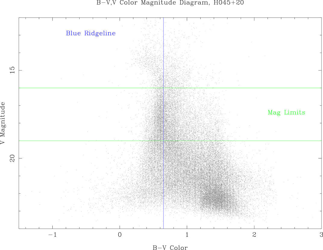
Figure 7: Example Color-Magnitude diagram in V and B-V for H045+20, observed using 90Prime. The magnitude range used in this analysis is bounded in green and the location of the “blue ridge” is shown in blue.

The fields used to test for triaxiality are circled on Figure 1 and listed in Table 6. For this initial analysis we use $V$ and the $B-V$ color only. A sample color-magnitude diagram for one of our fields is shown in Figure 7.

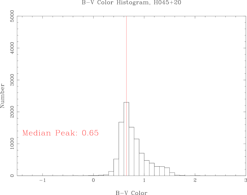
Figure 8: The number of stars vs. color for H045+20 for all stars with $16<V<19$ The location of the blue ridge line as determined by our median routine is indicated.

To isolate the faint blue stars in the Thick Disk/inner Halo which show the stellar excess, we use the easily recognized “blue ridge” which identifies the locus of the main sequence stars in each field. The green lines in Figure 7 delineate this magnitude range over which all of the Y4KCam and 90Prime fields are complete. At these magnitudes, a well-defined peak in the number of stars is apparent near $B-V\approx 0.6$, the blue ridge, as illustrated in the color histogram in Figure  8. As we have discussed in previous papers (Larsen & Humphreys, 1996; Parker et al., 2003), the GALMOD model shows that bluewards of this peak, we isolate a sample of inner halo and thick disk stars in the magnitude range $16<V<19$. Assuming that these are main sequence subdwarfs, these stars will be between 1 and 5 kpc from the Sun.

We define the peak of the blue ridge, $(B-V)_{P}$, as the median color of the stars within $\pm$ 0.4 dex of the maximum color bin, see Figure  8. The resulting blue ridge peak colors are included in Table 6. With the magnitude and color range thus defined, we also give the area of each field, the estimated completeness limit $V_{C}$, and the number of stars bluer than $(B-V)_{P}$ in the magnitude ranges $16<V<19$, $17<V<18$, and $18<V<19$.

We then determined the star count ratios for the paired fields in Q1 and Q4 normalizing for the area of the field. The ratios for each magnitude range are summarized in Table 7 with their error and the significance parameter, s computed as per Parker et al. (2003). The predicted ratios from GALMOD are also included. GALMOD ratios were required for all comparisons which involved fields above and below the plane because the Sun is not in the mid-plane of the disk but instead lies slightly above it (Humphreys & Larsen, 1995). Ratios of fields above the plane compared to fields below the plane should be slightly less than one due to this geometry and the Sun’s location in the Northern Galactic hemisphere. Comparisons between lines of sight in the same Galactic hemisphere should have a ratio near unity if the stellar distribution in the Galaxy is symmetric.

There are four comparisons in Table 7: Q1 and Q4 fields above the plane, Q1 and Q4 fields below the plane, Q1 fields above with those below the plane, and the Q4 fields above and below the plane.

We find a statistically significant excess in the ratios for the Q1 to Q4 fields above the plane for the two fields at the lowest longitudes, l of 45$\arcdeg$ and 50$\arcdeg$ that are an extension of the Hercules Thick Disk Cloud asymmetry. The fields at the greater longitudes, l of 55$\arcdeg$, 60$\arcdeg$, 65$\arcdeg$ and 75$\arcdeg$ show no trend of systematic deviations from a ratio of 1.0. For Q1 above and below the plane, there is a small excess above the plane in the two lowest longitude fields that does not extend to higher longitudes. We do not find evidence for an excess when comparing Q1 to Q4 below the plane or when comparing the Q4 fields above and below the plane. A few deviations from the expected ratios exist in isolated directions/magnitude bins and are of interest, but they do not show a systematic trend.

4 Summary and Conclusions – A Search for a Triaxial Thick Disk

Our star count ratios summarized in Table 7 show a small excess of faint blue stars at l of 45$\arcdeg$ and 50$\arcdeg$ but not at the greater longitudes including the faintest magnitude intervals. These results support Parker et al’s (2003) conclusion that the asymmetry feature in Q1 extends to about 55$\arcdeg$. We thus find no evidence that the Hercules Thick Disk Cloud and the star count excess is due to a triaxial Thick Disk. The ratios at l of 45$\arcdeg$ and 50$\arcdeg$ return to 1.0 at the faintest magnitude bin ($18<V<19$), suggesting that we may be seeing through the asymmetry feature; a possible clue to its extent along our line of sight in this direction. At $V\sim 19$ however, these faint blue stars will be about 2 kpc above the plane, and may not be in the Thick Disk.

We also note that the above vs. below the plane ratios in Q1 and Q4 and the Q1/Q4 ratio below the plane are consistent with the predictions of the Galactic model. There is no star count excess. This is not in agreement with Parker et al. (2003) who concluded that the excess exists both above and below the plane. This may be evidence that the Hercules Thick Disk Cloud is actually a debris stream. However, considering the small number of field pairs and the fact that we are apparently at the edge of the Cloud at these longitudes, we consider this a tentative result pending the analysis of the full set of fields.

Paper II will include an analysis of the full dataset, mapping the stellar excess in Galactic longitude and latitude and along the line of sight to determine the full extent of the Cloud. Our third paper will include the spectroscopy and analysis of the kinematics of the stars showing the excess.

Table 1: Field Information for the Thick Disk Asymmetry Project.

Field Name	$l$	$b$	Mean RA (J2000)	Mean Dec (J2000)	Instrument	Area	Run Observed
H020+20	20.63°	18.79°	17h17m12s	-01°46’31”	90Prime	1.04	2006 May
H020+32	20.53°	30.79°	16h35m28s	+04°09’44”	90Prime	1.04	2006 May
H020+47	20.30°	45.70°	15h42m32s	+11°17’18”	90Prime	0.77	2008 May
H020-47	21.02°	-48.25°	21h36m27s	-28°00’21”	Y4KCam	0.80	2008 Oct
H023+40	23.34°	38.69°	16h12m01s	+09°59’47”	90Prime	0.77	2008 May
H025+40	25.38°	38.83°	16h14m27s	+11°28’33”	90Prime	1.04	2006 May
H027+37	27.31°	35.72°	16h28m36s	+11°28’52”	90Prime	0.77	2008 May
H027-37	28.03°	-38.18°	20h59m56s	-20°22’32”	Y4KCam	0.80	2008 Oct
H027+40	27.25°	38.73°	16h17m24s	+12°44’26”	90Prime	0.77	2008 May
H030+20	30.51°	18.89°	17h34m43s	+06°29’21”	90Prime	1.04	2006 May
H030-20	30.90°	-21.17°	19h58m42s	-11°28’38”	90Prime	0.77	2007 Sep
H033+40	32.68°	38.76°	16h24m25s	+16°37’47”	90Prime	0.77	2008 May
H033-40	34.21°	-41.28°	21h19m20s	-17°02’39”	Y4KCam	0.48	2008 Oct
H035+32	35.34°	30.89°	16h58m07s	+15°34’43”	90Prime	1.04	2006 May
H035-32	36.06°	-33.06°	20h50m41s	-12°23’15”	90Prime	1.04	2006 May
H042-20	43.34°	-41.08°	21h30m28s	-10°43’38”	90Prime	0.77	2007 Sep
H042+40	42.09°	38.99°	16h34m08s	+23°35’27”	90Prime	1.04	2006 May
H042-40	43.30°	-41.07°	21h30m24s	-10°44’47”	90Prime	0.77	2007 Sep
H044+40	43.99°	38.92°	16h36m18s	+24°58’46”	90Prime	0.77	2008 May
H045+20	45.43°	19.02°	17h58m57s	+19°18’40”	90Prime	1.04	2006 May
H045-20	45.99°	-20.96°	20h24m20s	+01°04’50”	90Prime	1.04	2006 May
H046+45	45.08°	43.79°	16h16m17s	+27°02’01”	90Prime	0.77	2008 May
H048+45	47.27°	43.97°	16h17m05s	+28°36’35”	90Prime	0.77	2008 May
H050+31	50.23°	30.09°	17h20m37s	+27°19’10”	90Prime	1.04	2006 May
H050-31	51.19°	-31.87°	21h11m17s	-00°38’31”	90Prime	1.04	2006 May
H053+42	52.79°	41.05°	16h34m02s	+32°02’05”	90Prime	0.77	2008 May
H055+42	54.87°	41.20°	16h34m35s	+33°36’18”	90Prime	1.04	2006 May
H055-42	56.55°	-42.86°	21h57m14s	-03°16’54”	90Prime	0.59	2007 Sep
H060+20	60.32°	19.27°	18h21m40s	+32°25’12”	90Prime	1.04	2006 May
H060-20	61.06°	-20.69°	20h54m40s	+12°59’39”	90Prime	1.04	2006 May
H065+31	65.08°	30.36°	17h35m16s	+39°46’56”	90Prime	1.04	2006 May
H065-31	66.33°	-31.70°	21h41m43s	+09°44’33”	90Prime	0.78	2007 Sep
H075+20	75.28°	19.54°	18h45m52s	+45°44’02”	90Prime	1.04	2006 May
H075-20	76.14°	-20.50°	21h32m53s	+23°49’24”	90Prime	0.77	2007 Sep
H285-20	285.37°	-20.11°	08h11m31s	-72°10’17”	Y4KCam	0.70	2008 Oct
H285+20	286.13°	19.82°	11h23m00s	-39°45’21”	Y4KCam	0.90	2006 Apr
H295-31	294.94°	-31.35°	04h48m47s	-82°01’58”	Y4KCam	0.90	2008 Oct
H295+31	296.39°	30.60°	12h19m37s	-31°22’40”	Y4KCam	0.90	2006 Apr
H300-20	300.34°	-20.41°	11h28m40s	-82°19’09”	Y4KCam	0.85	2006 Apr
H300+20	301.12°	19.50°	12h36m33s	-42°47’15”	Y4KCam	0.90	2006 Apr
H305-42	304.75°	-42.67°	00h27m26s	-74°56’07”	Y4KCam	0.90	2008 Oct
H305+42	306.66°	41.38°	12h58m06s	-20°52’02”	90Prime	1.04	2006 May
H307+32	308.71°	41.23°	13h04m44s	-20°53’57”	90Prime	0.77	2008 May
H310+31	311.27°	30.30°	13h19m48s	-31°29’45”	Y4KCam	0.90	2006 Apr
H312+45	314.28°	44.14°	13h20m13s	-17°27’33”	90Prime	0.77	2008 May
H314+45	315.77°	44.09°	13h24m38s	-17°18’20”	90Prime	0.77	2008 May
H315-20	315.40°	-20.79°	16h51m22s	-76°49’47”	Y4KCam	0.90	2006 Apr
H315+20	316.13°	19.22°	13h52m43s	-41°26’05”	Y4KCam	0.90	2006 Apr
H316+40	317.52°	39.04°	13h34m48s	-21°56’24”	90Prime	0.77	2008 May
H318-40	318.02°	-41.07°	22h12m05s	-71°50’00”	Y4KCam	0.90	2008 Oct
H318+40	319.46°	39.17°	13h40m57s	-21°25’46”	90Prime	1.04	2006 May
H325-32	325.23°	-32.96°	20h10m13s	-70°11’34”	Y4KCam	0.90	2008 Oct
H325+32	326.19°	31.05°	14h15m31s	-27°16’07”	Y4KCam	0.92	2006 Apr
H327+40	328.88°	38.89°	14h10m41s	-19°12’19”	90Prime	0.77	2008 May
H330-20	330.46°	-21.01°	18h10m53s	-64°13’34”	Y4KCam	0.90	2006 Apr
H330+20	330.97°	18.98°	14h59m22s	-36°05’31”	Y4KCam	0.90	2006 Apr
H333-37	28.09°	-37.78°	20h58m26s	-20°11’59”	Y4KCam	0.21	2008 Oct
H333+37	334.20°	35.82°	14h32m34s	-20°03’01”	90Prime	0.77	2008 May
H333+40	334.30°	38.81°	14h26m45s	-17°23’50”	90Prime	0.77	2008 May
H335-20	335.09°	-41.24°	21h09m48s	-60°32’57”	Y4KCam	0.20	2008 Oct
H335-40	335.07°	-41.19°	21h09m26s	-60°34’26”	Y4KCam	0.53	2008 Oct
H335+40	336.19°	38.97°	14h31m47s	-16°32’02”	90Prime	1.04	2006 May
H337+40	338.24°	38.76°	14h37m54s	-15°52’59”	90Prime	0.77	2008 May
H340-20	340.52°	-21.09°	18h36m21s	-55°23’38”	Y4KCam	0.90	2006 Apr
H340+20	340.86°	18.91°	15h36m16s	-30°46’05”	Y4KCam	0.88	2006 Apr
H340+32	341.02°	30.87°	15h04m29s	-21°10’01”	90Prime	1.04	2006 May
H340+47	341.29°	45.75°	14h30m10s	-08°47’15”	90Prime	0.77	2008 May

Table 2: Mean extinction and color terms from the 90Prime camera on the Bok 2.3 meter telescope for May of 2006.

Band or Color	Atmospheric Extinction	Color Terms
$V$	$0.142\pm 0.024$	$-0.032\pm 0.010$
$BV$	$0.089\pm 0.011$	$1.125\pm 0.018$
$VR$	$0.049\pm 0.008$	$0.930\pm 0.010$
$UB$	$0.232\pm 0.009$	$0.957\pm 0.021$

Table 3: Mean extinction and color terms from the Y4KCam camera on the SMARTS 1.0 meter telescope for April of 2006.

Band or Color	Atmospheric Extinction	Color Terms
$V$	$0.163\pm 0.017$	$0.096\pm 0.013$
$BV$	$0.123\pm 0.007$	$0.847\pm 0.033$
$VR$	$0.052\pm 0.019$	$0.912\pm 0.025$
$UB$	$0.245\pm 0.030$	$0.877\pm 0.057$

Table 4: Star-Galaxy Separation Comparison between the JAL classifier and the Automated Plate Scanner for field H055+42. The table presents the number of classified stars (S) and galaxies (G) for each method along with the number of classifications in agreement. The last columns express the overall agreement and agreement on only the stellar classification between methods.

B Mag	APS	APS	JAL	JAL	Agree	Disagree	Agree	Disagree	Overall	Stellar
Range	S	G	S	G	G	G	S	S	Agreement	Agreement
15 - 16	4	0	3	1	0	1	3	0	75%	75%
16 - 17	74	2	73	3	1	2	72	1	96%	97%
17 - 18	377	33	388	22	10	12	365	23	91%	96%
18 - 19	635	82	653	64	45	19	616	37	92%	97%
19 - 20	432	191	499	124	110	14	415	81	84%	96%
20 - 21	234	241	345	130	110	19	213	131	68%	91%
21 - 22	137	194	264	67	55	12	123	139	54%	89%

Table 5: Star-Galaxy Separation Comparison between the JAL classifier and the Sloan Digital Sky Survey for field H055+42. The table presents the number of classified stars (S) and galaxies (G) for each method along with the number of classifications in agreement. The last columns express the overall agreement and agreement on only the stellar classification between methods.

B Mag	SDSS	SDSS	JAL	JAL	Agree	Disagree	Agree	Disagree	Overall	Stellar
Range	S	G	S	G	G	G	S	S	Agreement	Agreement
15 - 16	0	4	3	1	1	0	0	3	25%	0%
16 - 17	63	13	73	3	3	0	63	10	86%	100%
17 - 18	384	26	388	22	10	12	372	16	93%	96%
18 - 19	660	57	653	64	41	23	637	16	94%	96%
19 - 20	498	125	499	124	108	16	482	17	94%	96%
20 - 21	344	131	345	130	116	14	330	15	93%	95%
21 - 22	248	83	264	67	64	3	245	19	93%	98%

Table 6: Extinction Corrected Star Counts.

Field Name	Area	$V_{C}$	$(B-V)_{P}$	$16<V<19$	$17<V<18$	$18<V<19$
H045-20	1.02	21.0	0.70	3478	1241	1513
H045+20	1.02	21.0	0.65	3944	1465	1671
H050-31	1.02	21.0	0.64	1077	368	463
H050+31	1.02	20.7	0.68	1179	423	468
H055+42	1.02	20.5	0.61	547	154	260
H060-20	1.02	21.0	0.66	2689	949	521
H060+20	1.00	21.0	0.72	2803	1013	551
H065+31	1.01	20.5	0.70	937	342	354
H065-31	0.72	21.0	0.66	741	259	269
H075+20	1.02	21.0	0.67	2092	713	774
H075-20	0.77	19.3	0.65	1889	642	683
H285+20	0.93	19.6	0.65	1889	670	735
H285-20	0.73	19.0	0.63	1738	596	632
H295+31	0.93	19.4	0.59	890	299	383
H295-31	0.93	19.2	0.69	933	285	452
H300-20	0.93	18.5	0.58	2535	992	494
H300+20	0.93	19.2	0.62	2522	932	529
H305+42	1.02	21.0	0.64	525	170	242
H310+31	0.91	19.2	0.58	870	289	399
H315-20	0.93	19.4	0.58	3176	1052	1536
H315+20	0.93	19.5	0.58	2880	980	1418

Table 7: Star Count Ratios for fields with $|l|\geq 45-75\arcdeg$ from the Galactic Center.

Field	$l_{1}$/$l_{2}$	$b_{1}$/$b_{2}$	GALMOD Ratio Predictions			Observed Count Ratios
Ratio			$16<V<19$	$17<V<18$	$18<V<19$	$16<V<19$	$s$	$17<V<18$	$s$	$18<V<19$	$s$
Quadrant 1/Quadrant 4 ratios above the Galactic Plane
H045+20/H315+20	45/315	+20/+20	1.00	1.00	1.00	$1.25\pm 0.03$	8.12	$1.36\pm 0.06$	6.45	$1.07\pm 0.04$	1.92
H050+31/H310+31	50/310	+31/+31	1.00	1.00	1.00	$1.21\pm 0.05$	3.87	$1.31\pm 0.10$	3.07	$1.05\pm 0.07$	0.65
H055+42/H305+42	55/305	+42/+42	1.00	1.00	1.00	$1.04\pm 0.06$	0.66	$0.91\pm 0.10$	0.90	$1.07\pm 0.10$	0.70
H060+20/H300+20	60/300	+20/+20	1.00	1.00	1.00	$1.03\pm 0.03$	1.19	$1.01\pm 0.05$	0.24	$0.97\pm 0.06$	0.53
H065+31/H295+31	65/295	+31/+31	1.00	1.00	1.00	$0.97\pm 0.05$	0.67	$1.05\pm 0.08$	0.64	$0.85\pm 0.06$	2.37
H075+20/H285+20	75/285	+20/+20	1.00	1.00	1.00	$1.01\pm 0.03$	0.30	$0.97\pm 0.05$	0.57	$0.96\pm 0.05$	0.81
Quadrant 1/Quadrant 4 ratios below the Galactic Plane
H045-20/H315-20	45/315	-20/-20	1.00	1.00	1.00	$1.00\pm 0.02$	0.06	$1.08\pm 0.05$	1.68	$0.90\pm 0.03$	3.13
H060-20/H300-20	60/300	-20/-20	1.00	1.00	1.00	$0.97\pm 0.03$	1.23	$0.87\pm 0.04$	3.23	$0.96\pm 0.06$	0.64
H065-31/H295-31	65/295	-31/-31	1.00	1.00	1.00	$1.03\pm 0.03$	0.89	$1.02\pm 0.06$	0.37	$1.02\pm 0.06$	0.43
H075-20/H285-20	75/285	-20/-20	1.00	1.00	1.00	$1.03\pm 0.05$	0.51	$1.17\pm 0.10$	1.73	$0.77\pm 0.06$	3.91
Quadrant 1 ratios above/below the Galactic Plane
H045+20/H045-20	45/45	+20/-20	0.94	0.94	0.97	$1.13\pm 0.03$	6.33	$1.18\pm 0.05$	3.96	$1.10\pm 0.04$	3.25
H050+31/H050-31	50/50	+31/-31	0.97	0.97	0.98	$1.09\pm 0.05$	2.40	$1.15\pm 0.08$	2.25	$1.01\pm 0.07$	0.43
H060+20/H060-20	60/60	+20/-20	0.94	0.93	0.96	$0.99\pm 0.03$	1.66	$1.06\pm 0.05$	1.80	$1.07\pm 0.07$	1.85
H075+20/H075-20	75/75	+20/-20	0.94	0.93	0.96	$0.84\pm 0.05$	2.00	$0.84\pm 0.05$	1.80	$0.86\pm 0.04$	2.50
H065+31/H065-31	65/65	+31/-31	0.97	0.96	0.98	$0.90\pm 0.04$	1.75	$0.94\pm 0.08$	0.25	$0.94\pm 0.08$	0.50
Quadrant 4 ratios above/below the Galactic Plane
H315+20/H315-20	315/315	+20/-20	0.94	0.94	0.97	$0.91\pm 0.02$	1.50	$0.93\pm 0.04$	0.25	$0.92\pm 0.03$	1.60
H300+20/H300-20	300/300	+20/-20	0.94	0.93	0.96	$0.99\pm 0.03$	1.60	$0.94\pm 0.04$	0.25	$1.07\pm 0.07$	1.56
H285+20/H285-20	285/285	+20/-20	0.94	0.93	0.96	$0.85\pm 0.04$	2.25	$0.88\pm 0.05$	1.00	$0.91\pm 0.05$	1.00
H295+31/H295-31	295/295	+31/-31	0.97	0.96	0.98	$0.95\pm 0.04$	1.03	$1.05\pm 0.09$	1.00	$0.85\pm 0.06$	2.16

Figure 1: Distribution on the sky of project fields. Fields observed with 90Prime are plotted as open squared and fields observed with Y4KCam are represented as filled squares. Fields used for our first result on triaxiality are circled. The size of each icon is roughly twice as large as the actual sky coverage of the corresponding field.

Figure 5: Photometric comparison for H0055+42 between the 90Prime V band data and the SDSS DR5, converted to V band using the transformations of Rodgers et al. (2006).

References

- Abadi et al. (2003) Abadi, M. G., Navarro, J. F., Steinmetz, M., & Eke, V. R. 2003, ApJ, 597, 21
- Belokurov et al. (2007) Belokurov, V., et al. 2007, ApJ, 657, L89
- Benjamin et al. (2005) Benjamin, R. A., et al. 2005, ApJ, 630, L149
- Bernstein et al. (2002) Bernstein, R. A., Freedman, W. L., & Madore, B. F. 2002, ApJ, 571, 56
- Bertin & Arnouts (1996) Bertin, E., & Arnouts, S. 1996, A&AS, 117, 393
- Blitz & Spergel (1991) Blitz, L., & Spergel, D. N. 1991, ApJ, 379, 631
- Cabanela et al. (2003) Cabanela, J. E., Humphreys, R. M., Aldering, G., Larsen, J. A., Odewahn, S. C., Thurmes, P. M., & Cornuelle, C. S. 2003, PASP, 115, 837
- Cardelli et al. (1989) Cardelli, J. A., Clayton, G. C., & Mathis, J. S. 1989, ApJ, 345, 245
- Debattista & Sellwood (1998) Debattista, V. P., & Sellwood, J. A. 1998, ApJ, 493, L5
- Hammersley et al. (2000) Hammersley, P. L., Garzón, F., Mahoney, T. J., López-Corredoira, M., & Torres, M. A. P. 2000, MNRAS, 317, L45
- Hardie (1964) Hardie, R. H. 1964, Astronomical techniques, 178
- Hernquist & Weinberg (1992) Hernquist, L., & Weinberg, M. D. 1992, ApJ, 400, 80
- Humphreys & Larsen (1995) Humphreys, R. M., & Larsen, J. A. 1995, AJ, 110, 2183
- Ibata et al. (1994) Ibata, R. A., Gilmore, G., & Irwin, M. J. 1994, Nature, 370, 194
- Ibata & Gilmore (1995) Ibata, R. A., & Gilmore, G. F. 1995, MNRAS, 275, 591
- Ibata et al. (2001) Ibata, R., Irwin, M., Lewis, G. F., & Stolte, A. 2001, ApJ, 547, L133
- Ibata et al. (2003) Ibata, R. A., Irwin, M. J., Lewis, G. F., Ferguson, A. M. N., & Tanvir, N. 2003, MNRAS, 340, L21
- Jurić et al. (2008) Jurić, M., et al. 2008, ApJ, 673, 864
- Kazantzidis et al. (2008) Kazantzidis, S., Bullock, J. S., Zentner, A. R., Kravtsov, A. V., & Moustakas, L. A. 2008, ApJ, 688, 254
- Landolt (1992) Landolt, A. U. 1992, AJ, 104, 340
- Larsen & Humphreys (1996) Larsen, J. A., & Humphreys, R. M. 1996, ApJ, 468, L99
- Larsen & Humphreys (2003) Larsen, J. A., & Humphreys, R. M. 2003, AJ, 125, 1958
- Larsen et al. (2007) Larsen, J. A., et al. 2007, AJ, 133, 1247
- Larsen et al. (2008) Larsen, J. A., Humphreys, R. M., & Cabanela, J. E. 2008, ApJ, 687, L17
- Lasker et al. (1988) Lasker, B. M., et al. 1988, ApJS, 68, 1
- Lopez-Corredoira et al. (1997) Lopez-Corredoira, M., Garzon, F., Hammersley, P., Mahoney, T., & Calbet, X. 1997, MNRAS, 292, L15
- Majewski et al. (1999) Majewski, S. R., Siegel, M. H., Kunkel, W. E., Reid, I. N., Johnston, K. V., Thompson, I. B., Landolt, A. U., & Palma, C. 1999, AJ, 118, 1709
- Martin et al. (2004) Martin, N. F., Ibata, R. A., Conn, B. C., Lewis, G. F., Bellazzini, M., Irwin, M. J., & McConnachie, A. W. 2004, MNRAS, 355, L33
- Martínez-Delgado et al. (2005) Martínez-Delgado, D., Butler, D. J., Rix, H.-W., Franco, V. I., Peñarrubia, J., Alfaro, E. J., & Dinescu, D. I. 2005, ApJ, 633, 205
- Mink (1999) Mink, D. J. 1999, Astronomical Data Analysis Software and Systems VIII, 172, 498
- Monet et al. (2003) Monet, D. G., et al. 2003, AJ, 125, 984
- Newberg et al. (2002) Newberg, H. J., et al. 2002, ApJ, 569, 245
- Newberg et al. (2003) Newberg, H. J., et al. 2003, ApJ, 596, L191
- Odewahn et al. (1992) Odewahn, S. C., Stockwell, E. B., Pennington, R. L., Humphreys, R. M., & Zumach, W. A. 1992, AJ, 103, 318
- Odewahn et al. (1993) Odewahn, S. C., Humphreys, R. M., Aldering, G., & Thurmes, P. 1993, PASP, 105, 1354
- Osmer et al. (1998) Osmer, P. S., Kennefick, J. D., Hall, P. B., & Green, R. F. 1998, ApJS, 119, 189
- Parker et al. (2003) Parker, J. E., Humphreys, R. M., & Larsen, J. A. 2003, AJ, 126, 1346
- Parker et al. (2004) Parker, J. E., Humphreys, R. M., & Beers, T. C. 2004, AJ, 127, 1567
- Pence (1999) Pence, W. 1999, Astronomical Data Analysis Software and Systems VIII, 172, 487
- Rodgers et al. (2006) Rodgers, C. T., Canterna, R., Smith, J. A., Pierce, M. J., & Tucker, D. L. 2006, AJ, 132, 989
- Schlegel et al. (1998) Schlegel, D. J., Finkbeiner, D. P., & Davis, M. 1998, ApJ, 500, 525
- Stanek et al. (1994) Stanek, K. Z., Mateo, M., Udalski, A., Szymanski, M., Kaluzny, J., & Kubiak, M. 1994, ApJ, 429, L73
- Valdes (1998) Valdes, F. G. 1998, Astronomical Data Analysis Software and Systems VII, 145, 53
- Vivas et al. (2001) Vivas, A. K., et al. 2001, ApJ, 554, L33
- Weinberg (1992) Weinberg, M. D. 1992, ApJ, 384, 81
- Xu et al. (2007) Xu, Y., Deng, L. C., & Hu, J. Y. 2007, MNRAS, 379, 1373
- Yanny et al. (2003) Yanny, B., et al. 2003, ApJ, 588, 824