Two Weight Inequalities for Discrete Positive Operators

Abstract.

We characterize two weight inequalities for general positive dyadic operators. Let $\boldsymbol{\tau}=\{\tau_{Q}\;:\;Q\in\mathcal{Q}\}$ be non-negative constants associated to dyadic cubes, and define a linear operators by

$$\operatorname{T}_{\boldsymbol{\tau}}f \coloneqq\sum_{Q\in\mathcal{Q}}\tau_{Q}\cdot\mathbb{E}_{Q}f\cdot\mathbf{1}_{Q}\,.$$

Let $\sigma,\omega$ be non-negative locally finite weights on $\mathbb{R}^{d}$. We characterize the two weight inequalities

$$\lVert\operatorname{T}_{\boldsymbol{\tau}}(f\sigma)\rVert_{L^{q}(\omega)}\lesssim\lVert f\rVert_{L^{p}(\sigma)}\,,\qquad 1<p\leq q<\infty\,,$$

in terms of Sawyer-type testing conditions. For specific choices of constants $\tau_{Q}$, this reduces to the two weight fractional integral inequalities of Sawyer [MR930072]. The case of $p=q=2$, in dimension $1$, was characterized by Nazarov-Treil-Volberg [MR2407233], which result has found several interesting applications.

1. Introduction

Our interest is in extensions of the Carleson Embedding Theorem, especially in the discrete setting. We recall this well-known Theorem. Let $\mathcal{Q}$ be a choice of dyadic cubes in $\mathbb{R}^{d}$. For a cube $Q$, set

(1.1) $$\mathbb{E}_{Q}f\coloneqq\lvert Q\rvert^{-1}{\int_{Q}f\;dx}$$

Here we are abusing the probabilistic notation for conditional expectation.

1.2 Carleson Embedding Inequality.

Let $\{\tau_{Q}\;:\;\mathcal{Q}\}$ be non-negative constants, and let $1<p<\infty$. Define

(1.3) $$\lVert\tau_{Q}\rVert_{\textup{Car}}\coloneqq\sup_{Q\in\mathcal{Q}}\lvert Q\rvert^{-1}\sum_{\begin{subarray}{c}R\in\mathcal{Q}\\ R\subset Q\end{subarray}}\tau_{R}\,,$$

(1.4) $$C_{p}\coloneqq\sup_{\lVert f\rVert_{p}=1}\Bigl{[}\sum_{Q\in\mathcal{Q}}\tau_{Q}\lvert\mathbb{E}_{Q}f\rvert^{p}\Bigr{]}^{1/p}\,.$$

We have the equivalence $C_{p}\simeq\lVert\tau_{Q}\rVert_{\textup{Car}}^{1/p}$.

We are interested in weighted inequalities, especially two-weight inequalities, and in particular we will give discrete extensions of results of Sawyer [MR930072] (also see [MR1437584, MR1175693]) and Nazarov-Treil-Volberg [MR1685781]. For the study of such inequalities, it is imperative to have universal statements, universal in the weight, that can be applied to particular operators. By a weight we mean a non-negative locally integrable function $\omega\;:\;\mathbb{R}^{d}\to[0,\infty)$. While this is somewhat restrictive, by a limiting procedure, one can pass to more general measures. For such weights, and ‘nice’ sets like cubes $Q$ we will set

$$\omega(Q)\coloneqq\int_{Q}\omega\;dx\,.$$

A first operator that one can construct from a weight is the (dyadic) maximal function associated to $w$ given by

(1.5) $$\operatorname{M}_{\omega}f(x) \coloneqq\sup_{Q\in\mathcal{Q}}\mathbf{1}_{Q}(x)\mathbb{E}^{\omega}_{Q}\lvert f\rvert\,,$$

(1.6) $$\mathbb{E}^{\omega}_{Q}f \coloneqq\omega(Q)^{-1}\int_{Q}f\,\omega\;dx\,.$$

Here we are extending the definition in (1.1) to arbitrary weights. It is a basic fact, proved by exactly the same methods that proves the non-weighted inequality, that we have

1.7 Theorem.

We have the inequalities

(1.8) $$\lVert\operatorname{M}_{\omega}f\rVert_{L^{p}(\omega)}\lesssim\lVert f\rVert_{L^{p}(\omega)}\,,\qquad 1<p<\infty\,.$$

This, by exactly the same proof that proves the Carleson Embedding Theorem, gives us

1.9 Weighted Carleson Embedding Inequality.

Let $\{\tau_{Q}\;:\;\mathcal{Q}\}$ be non-negative constants, let $1<p<\infty$ and let $w$ be a weight. Define a weighted version of the Carleson norm by

(1.10) $$\lVert\tau_{Q}\rVert_{\textup{Car},w}\coloneqq\sup_{Q\in\mathcal{Q}}\omega(Q)^{-1}\sum_{\begin{subarray}{c}R\in\mathcal{Q}\\ R\subset Q\end{subarray}}\tau_{R}\,,$$

(1.11) $$C_{p,w}\coloneqq\sup_{\lVert f\rVert_{L^{p}(\omega)}=1}\Bigl{[}\sum_{Q\in\mathcal{Q}}\tau_{Q}\bigl{\lvert}\mathbb{E}_{Q}^{\omega}f\bigr{\rvert}^{p}\Bigr{]}^{1/p}\,.$$

We have the equivalence $C_{p,w}\simeq\lVert\tau_{Q}\rVert_{\textup{Car},w}^{1/p}$.

This is a foundational estimate in the two-weight theory, indeed the only tool needed for the proof of the two-weight maximal Theorem of Sawyer [MR676801].

We are concerned with the following deep extension, obtained by Nazarov-Treil-Volberg [MR1685781], of the Theorem of Eric Sawyer on two-weight inequalities for fractional integrals [MR930072].

1.12 Embedding Inequality of Sawyer and Nazarov-Treil-Volberg.

Let $\{\tau_{Q}\;:\;Q\in\mathcal{Q}\}$ be non-negative constants. Let $w,\sigma$ be weights. Define

(1.13) $$C_{1}^{2} \coloneqq\sup_{R}\sigma(R)^{-1}\int\Bigl{[}\sum_{Q\subset R}\tau_{Q}\mathbf{1}_{Q}\mathbb{E}_{Q}\sigma\Bigr{]}^{2}\omega\,,$$

(1.14) $$C_{2}^{2} \coloneqq\sup_{R}\omega(R)^{-1}\int\Bigl{[}\sum_{Q\subset R}\tau_{Q}\mathbf{1}_{Q}\mathbb{E}_{Q}w\Bigr{]}^{2}\sigma$$

(1.15) $$C_{3} \coloneqq\sup_{\lVert f\rVert_{L^{2}(\sigma)}=1}\sup_{\lVert g\rVert_{L^{2}(\omega)}=1}\sum_{Q\in\mathcal{Q}}\tau_{Q}\mathbb{E}_{Q}(f\sigma)\cdot\mathbb{E}_{Q}(g\omega)\cdot\lvert Q\rvert\,.$$

We have the equivalence $C_{3}\simeq C_{1}+C_{2}$.

The case of $\tau_{Q}=\lvert Q\rvert^{\alpha/d}$ for $0<\alpha<1$ corresponds to the result of Sawyer. Nazarov-Treil-Volberg identified the critical role of this result in two-weight inequalities. And it has been subsequently used in the proofs of several results, such as [MR2433959, MR2354322, MR2367098, MR1748283, MR1897458] among other papers.

The Nazarov-Treil-Volberg proof uses the Bellman Function approach. Our purpose is to give a new proof of this result, as well as extensions of it. In particular, our proof will work in all dimensions, a result that is new (but expected) in dimensions $d\geq 2$ and higher. We discuss the general case of $1<p\leq q<\infty$. We also focus on the quantitative versions of these Theorems, as such estimates are important for applications.

Let $\boldsymbol{\tau}=\{\tau_{Q}\;:\;Q\in\mathcal{Q}\}$ be non-negative constants, and define linear operators by

(1.16) $$\operatorname{T}_{\boldsymbol{\tau}}f \coloneqq\sum_{Q\in\mathcal{Q}}\tau_{Q}\cdot\mathbb{E}_{Q}f\cdot\mathbf{1}_{Q}\,,$$

(1.17) $$\operatorname{T}_{\boldsymbol{\tau},R}^{\textup{in}}f \coloneqq\sum_{\begin{subarray}{c}Q\in\mathcal{Q}\\ Q\subset R\end{subarray}}\tau_{Q}\cdot\mathbb{E}_{Q}f\cdot\mathbf{1}_{Q}\,,$$

(1.18) $$\operatorname{T}_{\boldsymbol{\tau},R}^{\textup{out}}f \coloneqq\sum_{\begin{subarray}{c}Q\in\mathcal{Q}\\ Q\supset R\end{subarray}}\tau_{Q}\cdot\mathbb{E}_{Q}f\cdot\mathbf{1}_{Q}$$

Here, we are defining the operator $T_{\alpha}$ and two different ‘localizations’ of $T_{\alpha}$ corresponding to a cube $R$, one local and the other global. With these definitions, we have the following equality:

(1.19) $$\operatorname{T}_{\boldsymbol{\tau}}f(x)=\operatorname{T}_{\boldsymbol{\tau},R}^{\textup{in}}f(x)+\operatorname{T}_{\boldsymbol{\tau},R^{(1)}}^{\textup{out}}f(x^{\prime})\,,\qquad x\in R\,\ x^{\prime}\in R^{(1)}\,.$$

Here and below, we will denote by $R^{(1)}$ the ‘parent’ of $R$: The minimal dyadic cube that strictly contains $R$. Note that the previous Theorem characterizes the inequality

(1.20) $$\lVert\operatorname{T}_{\boldsymbol{\tau}}(f\sigma)\rVert_{L^{2}(\omega)}\lesssim\lVert f\rVert_{L^{2}(\sigma)}$$

Below, we consider the $L^{p}(\sigma)$ to $L^{q}(\omega)$ mapping properties of $\operatorname{T}_{\boldsymbol{\tau}}$, where $1<p\leq q<\infty$. These inequalities are immediately translatable into bilinear embedding inequalities. First, we have the weak-type inequalities.

1.21 Theorem.

Let $\boldsymbol{\tau}$ be non-negative constants, and $w,\sigma$ weights. Let $1<p\leq q<\infty$. Define

(1.22) $$\llbracket\sigma,\omega\rrbracket_{\boldsymbol{\tau},p,q}^{\textup{Loc}} \coloneqq\sup_{R\in\mathcal{Q}}\omega(R)^{-1/q^{\prime}}\lVert\operatorname{T}_{\boldsymbol{\tau},R}^{\textup{in}}(\omega\mathbf{1}_{R})\rVert_{L^{p^{\prime}}(\sigma)}$$

(1.23) $$\llbracket\sigma,\omega\rrbracket_{\boldsymbol{\tau},p,q}^{\textup{Glo}} \coloneqq\sup_{R\in\mathcal{Q}}\omega(R)^{-1/q^{\prime}}\lVert\operatorname{T}_{\boldsymbol{\tau},R}^{\textup{out}}(\omega\mathbf{1}_{R})\rVert_{L^{p^{\prime}}(\sigma)}$$

We have the equivalence of norms below.

(1.24) $$\lVert\operatorname{T}_{\boldsymbol{\tau}}(\sigma\cdot)\rVert_{L^{p}(\sigma)\mapsto L^{q,\infty}(\omega)} \simeq\llbracket\sigma,\omega\rrbracket_{\boldsymbol{\tau},p,q}^{\textup{Loc}}\,,\qquad 1<p\leq q<\infty$$

(1.25) $$\lVert\operatorname{T}_{\boldsymbol{\tau}}(\sigma\cdot)\rVert_{L^{p}(\sigma)\mapsto L^{q,\infty}(\omega)} \simeq\llbracket\sigma,\omega\rrbracket_{\boldsymbol{\tau},p,q}^{\textup{Glo}}\,,\qquad 1<p<q<\infty\,.$$

Note that the first equivalence holds for $p\leq q$, while the second requires a strict inequality.

The ‘global conditions’, in (1.25) above and in (1.28) below, arise from the observations of Gabidzashvili and Kokilashvili [gk], also see [MR1791462]*Chapter 3 and [MR804116]. There is a corresponding, harder, strong-type characterization.

1.26 Theorem.

Under the same assumptions as Theorem 1.21 we have the equivalences of norms below.

(1.27) $$\lVert\operatorname{T}_{\boldsymbol{\tau}}(\sigma\cdot)\rVert_{L^{p}(\sigma)\mapsto L^{q}(\omega)} \simeq\llbracket\sigma,\omega\rrbracket_{\boldsymbol{\tau},p,q}^{\textup{Loc}}+\llbracket w,\sigma\rrbracket_{\boldsymbol{\tau},q^{\prime},p^{\prime}}^{\textup{Loc}}\,,\qquad 1<p\leq q<\infty$$

(1.28) $$\lVert\operatorname{T}_{\boldsymbol{\tau}}(\sigma\cdot)\rVert_{L^{p}(\sigma)\mapsto L^{q}(\omega)} \simeq\llbracket\sigma,\omega\rrbracket_{\boldsymbol{\tau},p,q}^{\textup{Glo}}+\llbracket w,\sigma\rrbracket_{\boldsymbol{\tau},q^{\prime},p^{\prime}.}^{\textup{Glo}}\,,\qquad 1<p<q<\infty\,.$$

In particular, the case of (1.27) with $p=q=2$ is Theorem 1.12.

We can take $\sigma$ and $w$ to be finite measures and $f$ a smooth Schwartz function, so that there are no convergence issues at any point of the arguments below. By $A\lesssim B$ we mean $A<KB$ for an absolute constant $K$. By $A\simeq B$ we mean $A\lesssim B$ and $B\lesssim A$. We will not try to keep track of constants that depend upon dimension, choices of $p,\,q$ or $\alpha$.

Acknowledgment.

Two of the authors completed part of this work while participating in a research program at the Centre de Recerca Matemática, at the Universitat Autònoma Barcelona, Spain. We thank the Centre for their hospitality, and very supportive environment.

2. Proof of the Weak-Type Inequalities

Throughout the proofs of both the strong and weak-type results, we will suppress the dependence of the operator $\operatorname{T}_{\boldsymbol{\tau}}=\operatorname{T}$ upon $\boldsymbol{\tau}=\{\tau_{Q}\}$.

2.1. Proof of the necessity of the testing conditions.

Let us assume the weak-type inequality on $\operatorname{T}$. Set $\mathfrak{N}\coloneqq\lVert\operatorname{T}(\sigma\cdot)\rVert_{L^{p}(\sigma)\mapsto L^{q,\infty}(\omega)}<\infty$. By duality for Lorentz spaces, we then have

$$\lVert\operatorname{T}(f\cdot\omega)\rVert_{L^{p^{\prime}}(\sigma)}\leq\mathfrak{N}\lVert f\rVert_{L^{q^{\prime},1}(\omega)}\,.$$

Apply this inequality to $f=\mathbf{1}_{Q}$ to see that

$$\lVert\operatorname{T}_{Q}(\mathbf{1}_{Q}\omega)\rVert_{L^{p^{\prime}}(\sigma)}\leq\lVert\operatorname{T}(\mathbf{1}_{Q}\omega)\rVert_{L^{p^{\prime}}(\sigma)}\leq\mathfrak{N}\omega(Q)^{1/q^{\prime}}\,.$$

Hence $\llbracket\sigma,\omega\rrbracket_{p,q}^{\textup{Loc}}\leq\mathfrak{N}$. For the global condition, note that

$$\omega(Q)^{-1/q^{\prime}}\lVert\operatorname{T}_{Q}^{\textup{out}}(\omega\mathbf{1}_{Q})\rVert_{L^{p^{\prime}}(\sigma)} \leq\mathfrak{N}\omega(Q)^{-1/q^{\prime}+1/q^{\prime}}=\mathfrak{N}\,.$$

Hence, $\llbracket\sigma,\omega\rrbracket_{p,q}^{\textup{Glo}}\leq\mathfrak{N}$.

2.2. Proof of the weak-type inequality assuming $\mathfrak{L}\coloneqq\llbracket\sigma,\omega\rrbracket_{p,q}^{\textup{Loc}}<\infty$.

We consider the proof that the ‘local testing condition’ implies the weak-type bound for $\operatorname{T}$.

Fix $f\in L^{p}(\sigma)$, smooth with compact support and $\lambda>0$. We bound the set $\{\operatorname{T}(f\sigma)>2\lambda\}$. Let $\mathcal{Q}_{\lambda}$ be the maximal dyadic cubes in $\{\operatorname{T}(f\sigma)>\lambda\}$ which also intersect the set $\{\operatorname{T}(f\sigma)>2\lambda\}$.

Let $Q^{(1)}$ denote the parent of a dyadic cube. For fixed $Q_{0}\in\mathcal{Q}_{\lambda}$, we must have that $Q_{0}^{(1)}$ contains a point $z$ with $\operatorname{T}(f\sigma)(z)<\lambda$. It follows that

$$\lambda >\operatorname{T}(f\sigma)(z)\geq\operatorname{T}_{Q_{0}^{(1)}}^{\textup{out}}(f\sigma)\,.$$

From this, we must have

(2.1) $$\lambda\leq\operatorname{T}_{Q_{0}}^{\textup{in}}(f\sigma)(x)\,,\qquad x\in Q_{0}\cap\{\operatorname{T}(f\sigma)(x)>2\lambda\}\,.$$

This represents an important localization of the operation $\operatorname{T}(f\sigma)$.

Note that we can estimate

(2.2) $$M \coloneqq\sum_{Q\in\mathcal{Q}_{\lambda}}\Bigl{[}\frac{1}{\omega(Q)}\int_{Q}\operatorname{T}_{Q}^{\textup{in}}(f\sigma)\omega\;dx\Bigr{]}^{q}\omega(Q)$$

(2.3) $$\lesssim\sum_{Q\in\mathcal{Q}_{\lambda}}\Bigl{[}\int_{Q}f\sigma\operatorname{T}_{Q}^{\textup{in}}(\mathbf{1}_{Q}\omega)\;dx\Bigr{]}^{q}\omega(Q)^{1-q}$$

(2.4) $$\lesssim\mathfrak{L}^{q}\sum_{Q\in\mathcal{Q}_{\lambda}}\Bigl{[}\int_{Q}\lvert f\rvert^{p}\sigma\Bigr{]}^{q/p}\omega(Q)^{q/q^{\prime}+1-q}$$

(2.5) $$\lesssim\mathfrak{L}^{q}\Bigl{[}\sum_{Q\in\mathcal{Q}_{\lambda}}\int_{Q}\lvert f\rvert^{p}\sigma\Bigr{]}^{q/p} (p\leq q)$$

(2.6) $$\lesssim\mathfrak{L}^{q}\lVert f\rVert_{L^{p}(\sigma)}^{q}\,.$$

Note that we have used duality to move the (self-dual) operator $\operatorname{T}_{\alpha}^{\textup{in}}$ over to the simpler function.

To complete the proof, we will split $\mathcal{Q}_{\lambda}$ into subcollections $\mathcal{E}$ and $\mathcal{F}$, where $\mathcal{E}$ consists of those cubes which are ‘empty’ of the set $\{\operatorname{T}(f\sigma)>2\lambda\}$, precisely for $\eta=2^{-q-1}$

$$\mathcal{E}\coloneqq\bigl{\{}Q\in\mathcal{Q}_{\lambda}\;:\;\omega(Q\cap\{\operatorname{T}(f\sigma)>2\lambda\})<\eta\omega(Q)\bigr{\}}\,,$$

and $\mathcal{F}=\mathcal{Q}_{\lambda}-\mathcal{E}$. And to conclude the proof, we can estimate, using (2.6),

$$(2\lambda)^{q}\omega(\operatorname{T}(f\sigma)>2\lambda) \leq\eta(2\lambda)^{q}\sum_{Q\in\mathcal{E}}\omega(Q)+\eta^{-q}M$$

$$\leq\eta 2^{q}\lambda^{q}\omega(\operatorname{T}(f\sigma)>\lambda)+C\eta^{-q}\mathfrak{L}^{q}\lVert f\rVert_{L^{p}(\sigma)}^{q}\,.$$

Take $\lambda$ so that the left-hand side of this inequality is close to maximal. (The supremum is a finite number by assumption.) By choice of $\eta$, this proves the estimate.

2.3. Proof of the weak-type inequality assuming $\mathfrak{G}\coloneqq\llbracket\sigma,\omega\rrbracket_{p,q}^{\textup{Glo}}<\infty$.

We show that the ‘global testing condition’ implies the weak-type inequality for the fractional integral operator, when $p<q$. This proof will depend upon a (clever) comparison to a maximal function. We proceed with the initial steps of the previous proof, up until (2.1).

We rewrite the sum in (2.1) in a way that permits our application of the ‘global’ testing condition. Inductively define $Q_{k}$ containing $x$ as follows. The cube $Q_{0}$ and $x$ are as (2.1) above, and given $Q_{k}\subset Q_{0}$, take $Q_{k+1}$ to be the maximal dyadic cube containing $x$ that satisfies $\omega(Q_{k+1})\leq\tfrac{1}{2}\omega(Q_{k})$. Then, we have, continuing from (2.1),

(2.7) $$\lambda \leq\sum_{k=0}^{\infty}\sum_{\begin{subarray}{c}Q\;:\;x\in Q\\ Q_{k+1}\subsetneqq Q\subset Q_{k}\end{subarray}}\tau_{Q}\lvert Q\rvert^{-1}\int_{Q}f\;\sigma dy$$

(2.8) $$\leq\sum_{k=0}^{\infty}\int_{Q_{0}}\Biggl{\{}\sum_{\begin{subarray}{c}Q\;:\;x\in Q\\ Q_{k+1}\subsetneqq Q\subset Q_{k}\end{subarray}}\tau_{Q}\lvert Q\rvert^{-1}\mathbf{1}_{Q}\Biggr{\}}f\;\sigma dy$$

(2.9) $$\lesssim\sum_{k=0}^{\infty}\int_{Q_{0}}\omega(Q^{(1)}_{k+1})^{-1}\operatorname{T}_{Q^{(1)}_{k+1}}^{\textup{out}}(\omega\mathbf{1}_{Q^{(1)}_{k+1}})\cdot(f\mathbf{1}_{Q_{k}})\;\sigma dy$$

(2.10) $$\lesssim\sum_{k=0}^{\infty}\omega(Q^{(1)}_{k+1})^{-1}\lVert\operatorname{T}_{Q^{(1)}_{k+1}}^{\textup{out}}(\omega\mathbf{1}_{Q^{(1)}_{k+1}})\rVert_{L^{p^{\prime}}(\sigma)}\Bigl{(}\int_{Q_{k}}f^{p}\sigma\Bigr{)}^{1/p}$$

(2.11) $$\lesssim\mathfrak{G}\sum_{k=0}^{\infty}\omega(Q^{(1)}_{k+1})^{-1/q}\Biggl{(}\int_{Q_{k}}f^{p}\;\sigma\Biggr{)}^{1/p}$$

(2.12) $$\lesssim\mathfrak{G}\sum_{k=0}^{\infty}\omega(Q_{k})^{1/p}\omega(Q^{(1)}_{k+1})^{-1/q}\Biggl{(}\omega(Q_{k})^{-1}\int_{Q_{k}}f^{p}\;\sigma\Biggr{)}^{1/p}$$

(2.13) $$\lesssim\mathfrak{G}\omega(Q_{0})^{1/p-1/q}\overline{\operatorname{M}}f(x)\,.$$

In the last inequality, we define the maximal function $\overline{\operatorname{M}}$ as follows.

$$\overline{\operatorname{M}}f(x)\coloneqq\sup_{Q\;:\;Q\subset Q_{0}}\mathbf{1}_{Q}(x)\Bigl{[}\omega(Q)^{-1}\int_{Q}f^{p}\;\sigma\Bigr{]}^{1/p}\,.$$

This is a localized maximal function, with both weights involved in the definition. In passing to (2.13), we should note that we are certainly using the strict inequality $p<q$: By construction, $\omega(Q^{(1)}_{k+1})\geq\tfrac{1}{2}\omega(Q_{k})$, so that

$$\sum_{k=0}^{\infty}\omega(Q_{k})^{1/p}\omega(Q^{(1)}_{k+1})^{-1/q} \lesssim\sum_{k=0}^{\infty}\omega(Q_{k})^{1/p-1/q}\lesssim\omega(Q_{0})^{1/p-1/q}\,.$$

The conclusion of these calculations is that for maximal dyadic $Q_{0}\subset\{\operatorname{T}(f\sigma)>\lambda\}$, and $x\in Q_{0}\cap\{\operatorname{T}(f\sigma)>2\lambda\}$, we have

$$\lambda\leq c\mathfrak{G}\omega(Q_{0})^{1/p-1/q}\overline{\operatorname{M}}f(x)\,.$$

We proceed with an estimate for $\omega(Q_{0}\cap\{\operatorname{T}(f\sigma)>2\lambda\})$.

Take $\mathcal{P}_{0}$ to be the maximal dyadic cubes $Q\subset Q_{0}$ so that

$$\lambda \leq c\mathfrak{G}\omega(Q_{0})^{1/p-1/q}\Biggl{[}\omega(Q)^{-1}\int_{Q}f^{p}\;\sigma\Biggr{]}^{1/p}\,,$$

$$\omega(Q) \leq c\mathfrak{G}^{p}\lambda^{-p}\omega(Q_{0})^{1-1/q}\int_{Q}f^{p}\;\sigma\,.$$

And this permits us to estimate

$$\lambda^{q}\omega\bigl{(}Q_{0}\cap\{\operatorname{T}(f\sigma)>2\lambda\}\bigr{)} \leq\lambda^{q}\sum_{Q\in\mathcal{P}_{0}}\omega(Q)$$

$$\lesssim\mathfrak{G}^{p}\lambda^{q-p}\omega(Q_{0})^{1-p/q}\sum_{Q\in\mathcal{Q}_{0}}\int_{Q}f^{p}\;\sigma$$

$$\lesssim\mathfrak{G}^{p}\lambda^{q-p}\omega(Q_{0})^{1-p/q}\int_{Q_{0}}f^{p}\;\sigma\,.$$

We have to this moment been working with a single maximal $Q_{0}\subset\{\operatorname{T}(f\sigma)>\lambda\}$ which also meets the set $\{\operatorname{T}(f\sigma)>2\lambda\}$. Let $\mathcal{Q}_{0}$ be the collection of all such $Q_{0}$. We can estimate

(2.14) $$(2\lambda)^{q}\omega(\operatorname{T}_{\alpha}(f\sigma)>2\lambda) \lesssim\mathfrak{G}^{p}\lambda^{q-p}\sum_{Q_{0}\in\mathcal{Q}_{0}}\omega(Q_{0})^{1-p/q}\int_{Q_{0}}f^{p}\;\sigma$$

(2.15) $$\lesssim\mathfrak{G}^{p}\lambda^{q-p}\Biggl{[}\sum_{Q_{0}\in\mathcal{Q}_{0}}\omega(Q_{0})\Biggr{]}^{1-p/q}\cdot\Biggl{[}\sum_{Q_{0}\in\mathcal{Q}_{0}}\Bigl{(}\int_{Q_{0}}f^{p}\sigma\Bigr{)}^{q/p}\Biggr{]}^{p/q}$$

(2.16) $$\lesssim\mathfrak{G}^{p}\bigl{[}\lambda^{q}\omega(\operatorname{T}(f\sigma)>\lambda)\bigr{]}^{1-p/q}\int f^{p}\;\sigma\,.$$

Apply (2.16) with a choice of $\lambda$ so that the left-hand side is close to maximal. It follows that we have

$$[\lambda^{q}\omega(\operatorname{T}_{\alpha}(f\sigma)>2\lambda)]^{p/q}\lesssim\mathfrak{G}^{p}\int f^{p}\;\sigma\,.$$

And this completes the proof.

3. Proof of Sawyer’s Two Weight Norm Result

3.1. Linearizations of Maximal Functions

The maximal theorem Theorem 1.7, giving universal bounds on the maximal function $\operatorname{M}_{\omega}$, will be an essential tool, arising in proof of the sufficiency of the testing conditions below. It will arise in a ‘linearized’ form. By this we mean the usual way to pass from a sub-linear maximal operator to a linear one, which for $\operatorname{M}_{\omega}$ means the following.

Let $\{E(Q)\;:\;Q\in\mathcal{Q}\}$ be any selection of measurable disjoint sets $E(Q)\subset Q$ indexed by the dyadic cubes. Define a corresponding linear operator $\operatorname{L}$ by

(3.1) $$\operatorname{L}f(x)\coloneqq\sum_{Q\in\mathcal{Q}}\mathbf{1}_{E(Q)}(x)\mathbb{E}^{\omega}_{Q}f\,.$$

Then, (1.8) is equivalent to the bound $\lVert\operatorname{L}f\rVert_{L^{p}(\omega)}\lesssim\lVert f\rVert_{L^{p}(\omega)}$ with implied constant independent of $w$ and the sets $\{E(Q)\;:\;Q\in\mathcal{Q}\}$.

3.2. Initial Considerations. Whitney Decomposition.

In this proof we will only explicitly use the ‘local’ testing conditions, which is sufficient to deduce the Theorem as the previous arguments show that the ‘local’ and ‘global’ conditions are equivalent, in the case of $1<p<q<\infty$. Let us set

(3.2) $$\mathfrak{L}\coloneqq\llbracket\sigma,\omega\rrbracket_{p,q}^{\textup{Loc}}\,,\qquad \mathfrak{L}_{\ast}\coloneqq\llbracket w,\sigma\rrbracket_{q^{\prime},p^{\prime}}^{\textup{Loc}}\,.$$

There is a very useful strengthening of the assumption that we can exploit, due to the fact that we have already proved the weak-type results, namely Theorem 1.21. Due to (1.24), we have

(3.3) $$\sup_{Q\in\mathcal{Q}}\omega(Q)^{-1/q^{\prime}}\lVert\operatorname{T}(\mathbf{1}_{Q}\omega)\rVert_{L^{p^{\prime}}(\sigma)}\lesssim\mathfrak{L}\,.$$

We take $f$ to be a finite combination of indicators of dyadic cubes. We work with the sets $\Omega_{k}=\{\operatorname{T}(f\sigma)>2^{k}\}$, which are open, and begin by making a Whitney-style decomposition of all of these sets.

Let $Q^{(1)}$ denote the parent of $Q$, and inductively define $Q^{(j+1)}=(Q^{(j)})^{(1)}$. For an integer $\rho\geq 2$, we should choose collections $\mathcal{Q}_{k}$ of disjoint dyadic cubes so that these several conditions are met.

(3.4) $$\Omega_{k}=\bigcup_{Q\in\mathcal{Q}_{k}}Q$$ (disjoint cover)

(3.5) $$Q^{(\rho)}\subset\Omega_{k}\,,\ Q^{(\rho+1)}\cap\Omega_{k}^{c}\neq\emptyset$$ (Whitney condition)

(3.6) $$\sum_{Q\in\mathcal{Q}_{k}}\mathbf{1}_{Q^{(\rho)}}\lesssim\mathbf{1}_{\Omega_{k}}$$ (finite overlap)

(3.7) $$\sup_{Q\in\mathcal{Q}_{k}}{}^{\sharp}\{Q^{\prime}\in\mathcal{Q}_{k}\;:\;Q^{\prime}\cap Q^{(\rho)}\neq\emptyset\}\lesssim 1\,,$$ (crowd control)

(3.8) $$Q\in\mathcal{Q}_{k}\,,\ Q^{\prime}\in\mathcal{Q}_{l}\,,\ Q\subsetneqq Q^{\prime}\quad\textup{implies }\quad k>l\,.$$ (nested property)

We will prove this for arbitrary $\rho$, but take $\rho=1$ in the proof.

Proof.

Take $\mathcal{Q}_{k}$ to be the maximal dyadic cubes $Q\subset\Omega_{k}$ which satisfy (3.5). Such cubes are disjoint and (3.4) holds. As the sets $\Omega_{k}$ are themselves nested, (3.8) holds.

Let us show that (3.6) holds. Note that holding the volume of the cubes constant we have

$$\sum_{\lvert Q\rvert=1}\mathbf{1}_{Q^{(\rho)}}\leq 2^{\rho d}$$

where $d$ is the dimension. So if we take an integer $\rho$, and assume that for some $k$ and $x\in\mathbb{R}^{d}$

$$\sum_{Q\in\mathcal{Q}_{k}}\mathbf{1}_{Q^{(\rho)}}(x)\geq 8\cdot 2^{(\rho+1)d}\,,$$

then we can choose $Q,R\in\mathcal{Q}_{k}$ with $x\in Q^{(\rho)}\cap R^{(\rho)}$ and the side-length of $R$ satisfies $\lvert R\rvert^{1/d}\leq 2^{-3}\lvert Q\rvert^{1/d}$. But then it will follow that $R^{(\rho+1)}\subset Q^{(\rho)}$. We thus see that $R^{(\rho+1)}$ does not meet $\Omega_{k}^{c}$, which is a contradiction.

Let us see that (3.7) holds. Fix $Q\in\mathcal{Q}_{k}$. If we had $Q^{\prime}\supsetneqq Q^{(\rho)}$ for any $Q^{\prime}\in\mathcal{Q}_{k}$, we would violate (3.5). Thus, we must have $Q^{\prime}\subset Q^{(\rho)}$, and these cubes Q’ are disjoint. Suppose that there were more than $2^{\rho+2}$ in number. Then, there would have to be a $Q^{\prime}\subset Q^{(\rho)}$ with $\lvert Q^{\prime}\rvert\leq 2^{-\rho-1}\lvert Q^{(\rho)}\rvert$. That is, $(Q^{\prime})^{(\rho+1)}\subset Q^{(\rho)}$, violating the Whitney condition (3.5).

∎

Let us comment on a subtle point that enters in a decisive way at the end of the proof, see Proposition 3.68. A given cube $Q$ can be a member of an unbounded number of $\mathcal{Q}_{k}$. Namely, there are integers $K_{-}(Q)\leq K_{+}(Q)$ so that

(3.9) $$Q\in\mathcal{Q}_{k}\,,\qquad K_{-}(Q)\leq k\leq K_{+}(Q)\,,$$

and there is no a priori upper bound on $K_{+}(Q)-K_{-}(Q)$.

3.3. Maximum Principle. Decomposition of $\lVert\operatorname{T}f\rVert_{L^{p}(\omega)}^{p}$.

There is an important maximum principle which will serve to further localize the operation $\operatorname{T}$. For all $k$ and $Q\in\mathcal{Q}_{k}$ we have

(3.10) $$\max\bigl{\{}\operatorname{T}_{Q^{(1)}}^{\textup{out}}(f\mathbf{1}_{Q^{(2)}}\sigma)(x)\,,\,\operatorname{T}(\mathbf{1}_{(Q^{(2)})^{c}}f\sigma)(x)\bigr{\}}\leq 2^{k}\,,\qquad x\in Q\,.$$

Proof.

We can choose $z\in Q^{(2)}\cap\Omega_{k}^{c}$, which exists by (3.5). Then, for $x\in Q$

$$\operatorname{T}(\mathbf{1}_{(Q^{(2)})^{c}}f\sigma)(x)=\operatorname{T}_{Q^{(1)}}^{\textup{out}}(\mathbf{1}_{(Q^{(2)})^{c}}f\sigma)(x)\leq\operatorname{T}(f\sigma)(z)\leq 2^{k}\,.$$

Also, it is clear that $\operatorname{T}_{Q^{(1)}}^{\textup{out}}(f\mathbf{1}_{Q^{(2)}}\sigma)(x)\leq\operatorname{T}(f\sigma)(z)\leq 2^{k}$. ∎

Let us set $m=5$. We will use this integer throughout the remainder of the proof. Define the sets

(3.11) $$E_{k}(Q)\coloneqq Q\cap(\Omega_{k+m-1}-\Omega_{k+m})\,,\qquad Q\in\mathcal{Q}_{k}\,.$$

It is required to include the subscript $k$ here, and in other places below, due to (3.9). See Figure 3.1 for an illustration of this set.

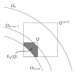
Figure 3.1. The set $E_{k}(Q)$.

Now, the Maximum Principle, the equality (1.19), and choice of $m$ gives us for $x\in E_{k}(Q)$

(3.12) $$\operatorname{T}_{Q^{(1)}}^{\textup{in}}(\mathbf{1}_{Q^{(2)}}f\sigma)(x) =\operatorname{T}(f\sigma)(x)-\operatorname{T}_{Q^{(1)}}^{\textup{out}}(f\mathbf{1}_{Q^{(2)}}\sigma)(x)-\operatorname{T}(\mathbf{1}_{(Q^{(2)})^{c}}f\sigma)(x)$$

(3.13) $$\geq 2^{k+m-1}-2^{k+1}\geq 2^{k}\,.$$

We should make one more observation. By the definition of $\operatorname{T}^{\textup{in}}$, we have

$$\operatorname{T}_{Q^{(1)}}^{\textup{in}}(\mathbf{1}_{Q^{(2)}}f\sigma)(x)=\operatorname{T}_{Q^{(1)}}^{\textup{in}}(\mathbf{1}_{Q^{(1)}}f\sigma)(x)\,,\qquad x\in Q\,.$$

On the right, we replace the cube $Q^{(2)}$ inside $\operatorname{T}$ with $Q^{(1)}$. This will be useful for us as it will, at a moment below, place the crowd control principle (3.7) at our disposal.

This permits us the following calculation which is basic to the organization of the proof.

(3.14) $$2^{k}\omega(E_{k}(Q)) \leq\int_{E_{k}(Q)}\operatorname{T}_{Q^{(1)}}^{\textup{in}}(\mathbf{1}_{Q^{(1)}}f\sigma)\;w$$

(3.15) $$=\int_{Q^{(1)}}f\cdot\operatorname{T}_{Q^{(1)}}^{\textup{in}}(\mathbf{1}_{E_{k}(Q)}\omega)\;\sigma$$

(3.16) $$=\alpha_{k}(Q)+\beta_{k}(Q)\,,$$

(3.17) $$\alpha_{k}(Q) \coloneqq\int_{Q^{(1)}\backslash\Omega_{k+m}}f\cdot\operatorname{T}_{Q^{(1)}}^{\textup{in}}(\mathbf{1}_{E_{k}(Q)}\omega)\;\sigma\,,$$

(3.18) $$\beta_{k}(Q) \coloneqq\int_{Q^{(1)}\cap\Omega_{k+m}}f\cdot\operatorname{T}_{Q^{(1)}}^{\textup{in}}(\mathbf{1}_{E_{k}(Q)}\omega)\;\sigma\,.$$

It is the term $\beta_{k}(Q)$ that leads to the (much) harder term.

And then, we can estimate

(3.19) $$\int\lvert\operatorname{T}(f\sigma)\rvert^{q}\;\omega \leq 2^{mq}\sum_{k=-\infty}^{\infty}2^{kq}\omega(\Omega_{k+m-1}-\Omega_{k+m})$$

(3.20) $$=2^{mq}\sum_{k=-\infty}^{\infty}\sum_{Q\in\mathcal{Q}_{k}}2^{kq}\omega(E_{k}(Q))$$

(3.21) $$=2^{mq}\sum_{j=1}^{3}S_{j}\,.$$

The last three sums are defined by a choice of $0<\eta<1$ and

(3.22) $$S_{j} \coloneqq\sum_{k=-\infty}^{\infty}\sum_{Q\in\mathcal{Q}_{k}^{j}}2^{kq}\omega(E_{k}(Q))\,,\qquad j=1,2,3\,,$$

(3.23) $$\mathcal{Q}_{k}^{1} \coloneqq\{Q\in\mathcal{Q}_{k}\;:\;\omega(E_{k}(Q))\leq\eta\omega(Q)\}\,,$$

(3.24) $$\mathcal{Q}_{k}^{2} \coloneqq\{Q\in\mathcal{Q}_{k}\;:\;\omega(E_{k}(Q))>\eta\omega(Q)\,,\ \alpha_{k}(Q)>\beta_{k}(Q)\}\,,$$

(3.25) $$\mathcal{Q}_{k}^{3} \coloneqq\mathcal{Q}_{k}-\mathcal{Q}_{k}^{1}-\mathcal{Q}_{k}^{2}\,.$$

Here, let us note that $\mathcal{Q}_{k}^{1}$ consists of those $Q\in\mathcal{Q}_{k}$ such that $E_{k}(Q)$ is ‘empty,’ and these terms will be handled much as they were in the weak-type argument. Using the notation of (3.9), observe that

(3.26) $$^{\sharp}\{K_{-}(Q)\leq k\leq K_{+}(Q)\;:\;Q\in\mathcal{Q}_{k}\backslash\mathcal{Q}_{k}^{1}\}\leq\eta^{-1}\,.$$

This follows from the definition of $\mathcal{Q}^{1}_{k}$, and that the sets $E_{k}(Q)$ are pairwise disjoint in $k$. This point enters in Proposition 3.68 below.

We will bound each of the $S_{j}$ in turn. In fact, recalling (3.2), we show that

(3.27) $$S_{1} \lesssim\eta\lVert\operatorname{T}(f\sigma)\rVert_{L^{q}(\omega)}^{q}$$

(3.28) $$S_{2} \lesssim\eta^{-q}\mathfrak{L}^{q}\lVert f\rVert_{L^{p}(\sigma)}^{q}$$

(3.29) $$S_{3} \lesssim\eta^{-q}\bigl{[}\mathfrak{L}^{q}+\mathfrak{L}_{\ast}^{q}\bigr{]}\lVert f\rvert\rVert_{L^{p}(\sigma)}^{q}\,.$$

Thus, the term $S_{2}$ requires the weak-type testing condition, while $S_{3}$ requires both testing conditions.

Figure 3.2. Schematic Tree for the proof of the strong type inequality.

This permits us to estimate

$$\int\lvert\operatorname{T}(f\sigma)\rvert^{q}\;\omega\lesssim\eta\cdot\lVert\operatorname{T}(f\sigma)\rVert_{L^{q}(\omega)}^{q}+\eta^{-q}\bigl{[}\mathfrak{L}^{q}+\mathfrak{L}_{\ast}^{q}\bigr{]}\cdot\lVert f\rvert\rVert_{L^{p}(\sigma)}^{q}\,.$$

The selection of $\eta$ is independent of the selection of $m$ (which is after all specified). So for small $0<\eta<1$, we can absorb the first term on the right into the left-hand side, proving our Theorem.

We include a schematic tree of the proof in Figure 3.2. Concerning this figure we make these comments.

• Terms in diamonds are further decomposed, while those in boxes are final estimates.

• The testing conditions used to control each final estimate are indicated on the edges. The label ‘absorb’ on $S_{1}$ indicates that this term is absorbed into the main term.

• $S_{3}$ is the hard term, requiring further decomposition, guided by the introduction of the ‘principal cubes,’ see Remark 3.47, and some delicate combinatorics, see Proposition 3.68.

3.4. Two Easy Estimates.

Now, the estimates (3.27) for $S_{1}$ and (3.28) for $S_{2}$ are reasonably straight forward, but more involved for $S_{3}$. Let us bound $S_{1}$. By the definition in (3.23), the sets $E_{k}(Q)$ are nearly empty.

(3.30) $$S_{1} =\sum_{k=-\infty}^{\infty}\sum_{Q\in\mathcal{Q}_{k}^{1}}2^{kq}\omega(E_{k}(Q))$$

(3.31) $$\leq\eta\sum_{k=-\infty}^{\infty}\sum_{Q\in\mathcal{Q}_{k}^{1}}2^{kq}\omega(Q)$$

(3.32) $$\leq\eta\sum_{k=-\infty}^{\infty}2^{kq}\omega(\{\operatorname{T}(f\sigma)>2^{k}\})$$

(3.33) $$\lesssim\eta\cdot\lVert\operatorname{T}(f\sigma)\rVert_{L^{q}(\omega)}^{q}$$

Here, we have used the condition (3.4).

Let us turn to $S_{2}$. The defining condition in (3.24) is that

$$\eta 2^{k}\omega(Q) \leq 2^{k}\omega(E_{k}(Q))$$

$$\lesssim\alpha_{k}(Q)$$

$$=\int_{Q^{(1)}\backslash\Omega_{k+m}}f\cdot\operatorname{T}_{Q^{(1)}}^{\textup{in}}(\mathbf{1}_{E_{k}(Q)}\omega)\;\sigma$$

$$\leq\Bigl{[}\int_{Q^{(1)}\backslash\Omega_{k+m}}f^{p}\;\sigma\Bigr{]}^{1/p}\cdot\Bigl{[}\int_{Q^{(1)}}\bigl{(}\operatorname{T}_{Q^{(1)}}^{\textup{in}}(\mathbf{1}_{E_{k}(Q)}\omega)\bigr{)}^{p^{\prime}}\;\sigma\Bigr{]}^{1/p^{\prime}}$$

$$\leq\mathfrak{L}\Bigl{[}\int_{Q^{(1)}\backslash\Omega_{k+m}}f^{p}\;\sigma\Bigr{]}^{1/p}\cdot\omega(Q)^{1/q^{\prime}}\,.$$

We have used the weak-type testing condition, and in particular (3.3). The estimate we use from this is

$$2^{k}\lesssim\mathfrak{L}\eta^{-1}\omega(Q)^{-1/q}\Bigl{[}\int_{Q^{(1)}\backslash\Omega_{k+m}}f^{p}\;\sigma\Bigr{]}^{1/p}\,.$$

Using this estimate, we can finish the estimate for $S_{2}$.

(3.34) $$S_{2} =\sum_{k=-\infty}^{\infty}\sum_{Q\in\mathcal{Q}_{k}^{2}}2^{kq}\omega(E_{k}(Q))$$

(3.35) $$\lesssim\eta^{-q}\mathfrak{L}^{q}\sum_{k=-\infty}^{\infty}\sum_{Q\in\mathcal{Q}_{k}^{2}}\frac{\omega(E_{k}(Q))}{\omega(Q)}\Bigl{[}\int_{Q^{(2)}\backslash\Omega_{k+m}}f^{p}\;\sigma\Bigr{]}^{q/p}$$

(3.36) $$\lesssim\eta^{-q}\mathfrak{L}^{q}\Bigl{[}\int f^{p}\sum_{k=-\infty}^{\infty}\sum_{Q\in\mathcal{Q}_{k}^{2}}\mathbf{1}_{Q^{(2)}\backslash\Omega_{k+m}}\;\sigma\Bigr{]}^{q/p}\qquad\qquad(q/p\geq 1)$$

(3.37) $$\lesssim\eta^{-q}\mathfrak{L}^{q}\Bigl{[}\int f^{p}\;\sigma\Bigr{]}^{q/p}\,.$$

Here, the $\Omega_{k}$ are decreasing sets, so the sum over $k$ above is bounded by $m=5$. This completes the proof of (3.28) for $S_{2}$.

3.5. The Difficult Case, Part 1.

We turn to the last and most difficult case, namely the estimate for (3.29). This subsection will introduce the essential tools for the analysis of this term, namely the collections $\mathcal{R}_{k}(Q)$ in (3.39) and the ‘principal cubes’ construction, see the paragraph around (3.43).

For integers $0\leq M<m$ we will show that

(3.38) $$S_{3,M}\coloneqq\sum_{\begin{subarray}{c}k\equiv M\;\textup{mod}m\end{subarray}}\sum_{Q\in\mathcal{Q}_{k}^{3}}2^{kq}\omega(E_{k}(Q))\lesssim\bigl{\{}\mathfrak{L}+\mathfrak{L}_{\ast}\bigr{\}}^{q}\eta^{-q}\lVert f\rVert_{L^{p}(\sigma)}^{q}\,,$$

where the implied constant is independent of $M$ and $N$. Summing over $M$ will prove (3.28) for $S_{3}$. It is the standing assumption for the remainder of the proof of (3.38) that $k\equiv M\mod m$.

This collection of cubes is important for us.

(3.39) $$\mathcal{R}_{k}(Q)\coloneqq\{R\in\mathcal{Q}_{k+m}\;:\;Q^{(1)}\cap R\neq\emptyset\}\,,\qquad Q\in\mathcal{Q}_{k}^{3}\,.$$

Recall that the set we are integrating over in $\beta_{k}(Q)$ is $Q^{(1)}\cap\Omega_{k+m}$, (3.18). Now, for $R\in\mathcal{R}_{k}(Q)$, we have $R\subset Q^{(1)}$. Indeed, if this is not the case, we have $Q^{(1)}\subsetneq Q^{(2)}\subset R\subset\Omega_{k+m}$, so that we have violated (3.5). Thus, we can write

$$Q^{(1)}\cap\Omega_{k+m}=\bigcup_{R\in\mathcal{R}_{k}(Q)}R\,.$$

In addition, for $R\in\mathcal{R}_{k}(Q)$, we must have that $R^{(1)}\subset\Omega_{k+m}$, by the Whitney condition (3.5). Hence $R^{(1)}\cap E_{k}(Q)=\emptyset$. See the definition of $E_{k}(Q)$ in (3.11). It follows that we have

(3.40) $$\mathbf{1}_{R}(x)\operatorname{T}_{Q^{(1)}}^{\textup{in}}(\mathbf{1}_{E_{k}(Q)}\omega)(x)=\mathbf{1}_{R}(x)\sum_{\begin{subarray}{c}P\in\mathcal{Q}\\ R^{(1)}\subsetneqq P\subset Q^{(1)}\end{subarray}}\tau_{P}\cdot\mathbb{E}_{P}(\mathbf{1}_{E_{k}(Q)}\omega)\,.$$

In particular, the right hand side is independent of $x\in R$. Putting these observations together, we see that

(3.41) $$\beta_{k}(Q) =\sum_{R\in\mathcal{R}_{k}(Q)}\int_{R}f\cdot\operatorname{T}_{Q^{(1)}}^{\textup{in}}(\mathbf{1}_{E_{k}(Q)}\omega)\;\sigma$$

(3.42) $$=\sum_{R\in\mathcal{R}_{k}(Q)}\int_{R}\operatorname{T}_{Q^{(1)}}^{\textup{in}}(\mathbf{1}_{E_{k}(Q)}\omega)\;\sigma\cdot\mathbb{E}_{R}^{\sigma}f\,.$$

The maximal function $\operatorname{M}_{\sigma}f$ has appeared in the last display, in the guise of the average $\mathbb{E}_{R}^{\sigma}f$. We proceed with the construction of the so-called ‘principal cubes.’ This construction consists of a subcollection $\mathcal{G}\subset\bigcup_{\begin{subarray}{c}k\equiv M\;\textup{mod}m\\ k\geq-N\end{subarray}}\mathcal{Q}_{k}$ satisfying these two properties:

(3.43) $$\forall\ Q\in\bigcup_{\begin{subarray}{c}k\equiv M\;\textup{mod}m\\ k\geq-N\end{subarray}}\mathcal{Q}_{k}\ \ \exists G\in\mathcal{G}\quad\textup{so that }\quad Q\subset G\quad\textup{and}\quad\mathbb{E}_{Q}^{\sigma}f\leq 2\mathbb{E}_{G}^{\sigma}f\,,$$

(3.44) $$G,G^{\prime}\in\mathcal{G}\,,\ G\subsetneqq G^{\prime}\ \quad\textup{implies}\quad 2\mathbb{E}_{G^{\prime}}^{\sigma}f<\mathbb{E}_{G}^{\sigma}f\,.$$

It is easy to recursively construct this collection. Let $\Gamma(Q)$ be the minimal element of $\mathcal{G}$ which contains it. (So $\Gamma(Q)$ is the ‘father’ of $Q$ in the collection $\mathcal{G}$.) It follows by construction that $\mathbb{E}_{Q}^{\sigma}f\leq 2\mathbb{E}_{\Gamma(Q)}^{\sigma}f$ for all $Q$. A basic property of this construction, which we rely upon below is that

(3.45) $$\sum_{G\in\mathcal{G}}\mathbf{1}_{G}(x)\mathbb{E}_{G}^{\sigma}f\lesssim\operatorname{M}_{\sigma}f(x)\,.$$

Indeed, for each fixed $x$, the terms in the series on the left are growing at least geometrically, by (3.44), whence the sum on the left is of the order of its largest term, proving the inequality. It follows from (3.1), that we have

(3.46) $$\sum_{G\in\mathcal{G}}\sigma(G)\lvert\mathbb{E}_{G}^{\sigma}f\rvert^{p}\lesssim\lVert f\rVert_{L^{p}(\sigma)}^{p}\,.$$

Both of these facts will be used below.

3.47 Remark.

Sawyer’s paper on the fractional integrals [MR930072] attributes this construction to Muckenhoupt and Wheeden [MR0447956]. In the intervening years, very similar constructions have been used many times, to mention just a few references, see these papers, which frequently use the words ‘corona decomposition:’ David and Semmes [MR1251061, MR1113517], which discuss the use of singular integrals in the context of rectifability. Consult the corona decomposition in [MR2179730], and the paper [MR1934198] includes several examples in the context of dyadic analysis. Its use in weighted inequalities appears in [0906.1941].

3.48 Remark.

It is an important point that the inequality (3.44) cannot be reversed. Indeed, the measure $\sigma$ is arbitrary, whence the averages $\mathbb{E}_{G}^{\sigma}f$ can increase dramatically as one passes from larger principal cubes to smaller principal cubes.

We can now make a further estimate of $\beta_{k}(Q)$. Let us set $\mathcal{N}_{k}(Q)=\{Q^{\prime}\in\mathcal{Q}_{k}\;:\;Q^{\prime}\cap Q^{(1)}\neq\emptyset\}$. (These are the ‘neighbors’ of $Q$ in the collection $\mathcal{Q}_{k}$.) The basic fact, a consequence of the crowd control property (3.7), is that

(3.49) $$\sharp\mathcal{N}_{k}(Q)\lesssim 1\,.$$

Continuing from (3.42), we derive a particular consequence of the construction of $\mathcal{G}$ as a subset of the Whitney cubes. Namely, for $Q\in\mathcal{Q}_{k}$, and $R\in\mathcal{R}_{k}(Q)\subset\mathcal{Q}_{k+m}$, we necessarily have $R\subset Q^{\prime}_{R}$ for a unique $Q^{\prime}_{R}\in\mathcal{N}_{k}(Q)$. And, we have that $\Gamma(R)=\Gamma(Q^{\prime}_{R})$ or $R\in\mathcal{G}$. This permits us to estimate

(3.50) $$\beta_{k}(Q) \leq\sum_{R\in\mathcal{R}_{k}(Q)}\int_{R}\operatorname{T}_{Q^{(1)}}^{\textup{in}}(\mathbf{1}_{E_{k}(Q)}\omega)\;\sigma\cdot\mathbb{E}_{R}^{\sigma}f$$

(3.51) $$\leq\beta_{k,4}(Q)+\beta_{k,5}(Q)\,,$$

(3.52) $$\beta_{k,4}(Q) \coloneqq\sum_{\begin{subarray}{c}R\in\mathcal{R}_{k}(Q)\\ \Gamma(R)=\Gamma(Q^{\prime}_{R})\end{subarray}}\int_{R}\operatorname{T}(\mathbf{1}_{Q}\omega)\;\sigma\cdot\mathbb{E}_{R}^{\sigma}f$$

(3.53) $$\beta_{k,5}(Q) \coloneqq\sum_{\begin{subarray}{c}{R\in\mathcal{R}_{k}(Q)}\\ R\in\mathcal{G}\end{subarray}}\int_{R}\operatorname{T}(\mathbf{1}_{Q}\omega)\;\sigma\cdot\mathbb{E}_{R}^{\sigma}f\,.$$

We have replaced $\operatorname{T}_{Q^{(1)}}^{\textup{in}}(\mathbf{1}_{E_{k}(Q)}\omega)$ by the larger term $\operatorname{T}(\omega\mathbf{1}_{Q})$.

We use the defining condition of $\mathcal{Q}_{k}^{3}$, recall (3.25), which gives us

$$\eta 2^{k}\omega(Q) \leq 2^{k}\omega(E_{k}(Q))\leq\beta_{k}(Q)\,,$$

$$\textup{whence}\qquad 2^{k} \lesssim\frac{\beta_{k}(Q)}{\eta\omega(Q)}\,.$$

Thus, our estimate of the term in (3.38), $S_{3,M}$ is given by

(3.54) $$S_{3,M} \lesssim\eta^{-q}\bigl{[}S_{4,M}+S_{5,M}\bigr{]}$$

(3.55) $$S_{v,M} \coloneqq\sum_{\begin{subarray}{c}k\equiv M\mod m\end{subarray}}\sum_{Q\in\mathcal{Q}_{k}^{3}}\frac{\omega(E_{k}(Q))}{\omega(Q)^{q}}\beta_{k,v}(Q)^{q}\qquad v=4,5\,.$$

We estimate these last two terms separately.

3.6. The Difficult Case, Part 2.

Let us fix a $G\in\mathcal{G}$, that is one of the principal cubes, and define

$$S_{k,4}^{\prime}(Q,G) \coloneqq\frac{\omega(E_{k}(Q))}{\omega(Q)^{q}}\Biggl{[}\sum_{\begin{subarray}{c}R\in\mathcal{R}_{k}(Q)\\ \Gamma(R)=\Gamma(Q^{\prime}_{R})=G\end{subarray}}\int_{R}\operatorname{T}(\mathbf{1}_{Q}\omega)\;\sigma\cdot\mathbb{E}_{R}^{\sigma}f\Biggr{]}^{q}$$

$$\lesssim(\mathbb{E}_{G}^{\sigma}f)^{q}{\omega(E_{k}(Q))}\Biggl{[}\omega(Q)^{-1}\sum_{\begin{subarray}{c}R\in\mathcal{R}_{k}(Q)\\ \Gamma(R)=\Gamma(Q^{\prime}_{R})=G\end{subarray}}\int_{R}\operatorname{T}(\mathbf{1}_{Q}\omega)\;\sigma\Biggr{]}^{q}$$

$$\lesssim(\mathbb{E}_{G}^{\sigma}f)^{q}{\omega(E_{k}(Q))}\Bigl{[}\omega(Q)^{-1}\int_{Q^{\prime}}\operatorname{T}(\mathbf{1}_{Q}\omega)\;\sigma\Bigr{]}^{q}$$

$$\lesssim(\mathbb{E}_{G}^{\sigma}f)^{q}{\omega(E_{k}(Q))}\Bigl{[}\omega(Q)^{-1}\int_{Q}\operatorname{T}(\mathbf{1}_{Q^{\prime}}\sigma)\;\omega\Bigr{]}^{q} (\textup{duality})$$

$$\lesssim(\mathbb{E}_{G}^{\sigma}f)^{q}{\omega(E_{k}(Q))}\Bigl{[}\omega(Q)^{-1}\int_{Q}\operatorname{T}(\mathbf{1}_{G}\sigma)\;\omega\Bigr{]}^{q} (\mathbf{1}_{Q^{\prime}}\leq\mathbf{1}_{G})$$

In the last line, we have replaced $\mathbf{1}_{Q^{\prime}}$ by the larger $\mathbf{1}_{G}$, since $Q^{\prime}\subset G$, as $\Gamma(Q^{\prime})=G$.

The sets $E_{k}(Q)$ are themselves disjoint, so that the sum above itself arises from a linearization of the maximal function $\operatorname{M}_{\omega}$. And we can estimate, again for fixed $G\in\mathcal{G}$,

$$\sum_{k}\sum_{Q\in\mathcal{Q}_{k}}S_{k,4}^{\prime}(Q,G) \leq(\mathbb{E}_{G}^{\sigma}f)^{q}\sum_{k}\sum_{Q\in\mathcal{Q}_{k}}{\omega(E_{k}(Q))}\Bigl{[}\omega(Q)^{-1}\int_{Q}\operatorname{T}(\mathbf{1}_{G}\sigma)\;\omega\Bigr{]}^{q}$$

$$\lesssim(\mathbb{E}_{G}^{\sigma}f)^{q}\int\operatorname{M}_{\omega}(\operatorname{T}(\mathbf{1}_{G}\sigma))^{q}\;\omega$$

$$\lesssim(\mathbb{E}_{G}^{\sigma}f)^{q}\int\operatorname{T}(\mathbf{1}_{G}\sigma)^{q}\;\omega$$

$$\lesssim\mathfrak{L}_{\ast}^{q}(\mathbb{E}_{G}^{\sigma}f)^{q}\sigma(G)^{q/p}\,.$$

Here we have used $L^{q}(\omega)$ bound on $\operatorname{M}_{\omega}$, the dual testing condition, and the analog of (3.3) for $\mathfrak{L}_{\ast}$, which holds since we have already established the weak-type Theorem.

Combining these last two estimates, observe that we have the following estimate.

(3.56) $$S_{4,M} =\sum_{G\in\mathcal{G}}\sum_{k}\sum_{Q\in\mathcal{Q}_{k}}S^{\prime}_{k,4}(Q,G)$$

(3.57) $$\lesssim\mathfrak{L}_{\ast}^{q}\sum_{G\in\mathcal{G}}(\mathbb{E}_{G}^{\sigma}f)^{q}\sigma(G)^{q/p}$$

(3.58) $$\lesssim\mathfrak{L}_{\ast}^{q}\Bigl{[}\sum_{G\in\mathcal{G}}(\mathbb{E}_{G}^{\sigma}f)^{p}\sigma(G)\Bigr{]}^{q/p} (q/p\leq 1)$$

(3.59) $$\lesssim\mathfrak{L}_{\ast}^{q}\lVert f\rVert_{L^{p}(\sigma)}^{q}\,.$$

The last line follows from (3.46). This completes the estimate for $S_{4,M}$.

3.7. The Difficult Case, Part 3.

It remains to bound $S_{5,M}$, with $\beta_{k,5}(Q)$ as defined in (3.53). With an abuse of notation we are going to denote the summand in the definition of $S_{5,M}$, see (3.55), as follows.

(3.60) $$\beta_{k,6}(Q) \coloneqq\frac{\omega(E_{k}(Q))}{\omega(Q)^{q}}\Biggl{[}\sum_{\begin{subarray}{c}{R\in\mathcal{R}_{k}(Q)}\\ R\in\mathcal{G}\end{subarray}}\int_{R}\operatorname{T}(\mathbf{1}_{Q}\omega)\;\sigma\cdot\mathbb{E}_{R}^{\sigma}f\Biggr{]}^{q}$$

(3.61) $$\lesssim\beta_{k,7}(Q)\cdot\beta_{k,8}(Q)\,,$$

(3.62) $$\beta_{k,7}(Q) \coloneqq\frac{\omega(E_{k}(Q))}{\omega(Q)^{q}}\Biggl{[}\sum_{\begin{subarray}{c}{R\in\mathcal{R}_{k}(Q)}\\ R\in\mathcal{G}\end{subarray}}\sigma(R)^{-p^{\prime}/p}\Biggl{(}\int_{R}\operatorname{T}(\mathbf{1}_{Q}\omega)\;\sigma\Biggr{)}^{p^{\prime}}\Biggr{]}^{q/p^{\prime}}\,,$$

(3.63) $$\beta_{k,8}(Q) \coloneqq\Biggl{[}\sum_{\begin{subarray}{c}{R\in\mathcal{R}_{k}(Q)}\\ R\in\mathcal{G}\end{subarray}}\sigma(R)\cdot(\mathbb{E}_{R}^{\sigma}f)^{p}\Biggr{]}^{q/p}\,.$$

Here, we have introduced the terms $\sigma(Q^{\prime})^{\pm 1/p}$, and used the Hölder inequality in the $\ell^{p}$–$\ell^{p^{\prime}}$ norms.

Our first observation that the terms $\beta_{k,7}(Q)$ admit a uniform bound. On the right in (3.62), we use the trivial bound $\omega(E_{k}(Q))\leq\omega(Q)$, and push the $p^{\prime}$ inside the integral to place ourselves in a position where we can appeal to the dual testing condition, namely (3.3).

$$\beta_{k,7}(Q) \lesssim\frac{1}{\omega(Q)^{q-1}}\Biggl{[}\sum_{\begin{subarray}{c}{R\in\mathcal{R}_{k}(Q)}\\ R\in\mathcal{G}\end{subarray}}\int_{R}\operatorname{T}(\mathbf{1}_{Q}\omega)^{p^{\prime}}\;\sigma\Biggr{]}^{q/p^{\prime}}$$

$$\lesssim\frac{1}{\omega(Q)^{q-1}}\lVert\operatorname{T}(\mathbf{1}_{Q}\omega)\rVert_{L^{p^{\prime}}(\sigma)}^{q}$$

$$\lesssim\mathfrak{L}^{q}\frac{\omega(Q)^{q/q^{\prime}}}{\omega(Q)^{q-1}}$$

$$\lesssim\mathfrak{L}^{q}\,.$$

It follows from (3.55) and (3.61) that we have

(3.64) $$S_{5,M} \lesssim\mathfrak{L}^{q}\sum_{k}\sum_{Q\in\mathcal{Q}_{k}^{3}}\beta_{k,8}(Q)$$

(3.65) $$\lesssim\mathfrak{L}^{q}\Biggl{[}\sum_{k}\sum_{Q\in\mathcal{Q}_{k}^{3}}\beta_{k,8}(Q)^{p/q}\Biggr{]}^{q/p} (p\leq q)$$

(3.66) $$\lesssim\mathfrak{L}^{q}\Biggl{[}\sum_{k}\sum_{Q\in\mathcal{Q}_{k}^{3}}\sum_{\begin{subarray}{c}{R\in\mathcal{R}_{k}(Q)}\\ R\in\mathcal{G}\end{subarray}}\sigma(R)\cdot(\mathbb{E}_{R}^{\sigma}f)^{p}\Biggr{]}^{q/p}\,.$$

At this point, a subtle point arises. The cubes $R\in\mathcal{R}_{k}(Q)\subset\mathcal{Q}_{k+m}$, but a given cube $R$ can potentially arise in many $\mathcal{Q}_{k+m}$, as we noted in (3.9). A given $R$ can potentially arise in the sum above many times, however this possibility is excluded by Proposition 3.68 below. In particular, we can continue the estimate above as follows.

(3.67) $$\eqref{e.S5<} \lesssim\mathfrak{L}^{q}\Biggl{[}\sum_{G\in\mathcal{G}}\sigma(G)(\mathbb{E}_{G}^{\sigma}f)^{p}\Biggr{]}^{q/p}\lesssim\mathfrak{L}^{q}\lVert f\rVert_{L^{p}(\sigma)}^{q}\,,$$

with the last inequality following from (3.46). The proof of Theorem 1.26 is complete, aside from the next proposition.

3.68 Proposition.

[Bounded Occurrences of $R$] Fix a cube $R$, and for $1\leq\ell\leq L$ suppose that

1. there is an integer $k(\ell)$ and $Q_{\ell}\in\mathcal{Q}_{k(\ell)}^{3}$ with $R\in\mathcal{R}_{k(\ell)}(Q)$,

2. the pairs $(Q_{\ell},k(\ell))$ are distinct.

We then have that $L\lesssim 1$, with the implied constant depending upon $1$, dimension, and $\eta$, the small constant that enters the proof at (3.23)—(3.25).

Proof.

There are two principal obstructions to the Lemma being true: (1) It could occur, after a potential reordering that $Q_{1}\subsetneq Q_{2}\subsetneq\cdots\subsetneq Q_{L}$. (2) It could happen that $Q_{1}=\cdots=Q_{L}$ but the $k_{\ell}$ are distinct. We treat these two obstructions in turn.

Fix $R$. We have see that $R\subset Q^{(1)}_{\ell}$ for all $1\leq\ell\leq L$, see the paragraph after (3.39). Suppose we have $R\subset Q^{(1)}_{\ell_{1}}\subsetneq Q^{(1)}_{\ell_{2}}$ with $k(\ell_{1})<k(\ell_{2})$. This would violate the Whitney condition (3.5).

Let us now consider the obstruction (1) above, namely after a relabeling, we have $k(1)>k(2)>\cdots>k({m+2})$, and

$$R\subset Q^{(1)}_{k(1)}\subsetneq Q^{(1)}_{k(2)}\subsetneq Q^{(1)}_{k(3)}\subsetneq\cdots\subsetneq Q^{(1)}_{k({m+2})}$$

This implies that $R\in\mathcal{Q}_{k(1)+m}$ and $R\in\mathcal{Q}_{k({m+2})+m}$, so that again by the nested property, $R\in\mathcal{Q}_{k}$ for all $k({m+2})+m\leq k\leq k(1)+m$. Therefore, for $s=m+2$ we have $R,Q_{s}\in\mathcal{Q}_{s}$ and $R^{(2)}\subset Q_{s}^{(1)}$. That is, $R$ violates the Whitney condition (3.5), a contradiction.

We conclude that there are only a bounded number of positions for the cube $Q_{\ell}^{(1)}$, and hence a bounded number of positions for the cubes $Q_{\ell}$. Thus, after a pigeonhole argument, and relabeling, we are concerned with the obstruction (2) above. We can after a relabeling, add to the conditions (1) and (2) in the Proposition that there is a fixed cube $\overline{Q}$ with $Q_{\ell}=\overline{Q}$ for $1\leq\ell\leq L^{\prime}$, and have $L\lesssim L^{\prime}$. This means in particular that the $k_{\ell}$ are distinct.

The defining condition, (3.25), that $\overline{Q}\in\mathcal{Q}_{k_{\ell}}^{3}$ means in particular that we have $\omega(E_{k_{\ell}}(\overline{Q}))>\eta\omega(\overline{Q})$. But, the condition that the $k_{\ell}$ be distinct means that the sets $E_{k_{\ell}}(\overline{Q})$ are distinct, hence $L^{\prime}\leq\eta^{-1}$ and our proof is finished.

∎

AuscherP.HofmannS.MuscaluC.TaoT.ThieleC.Carleson measures, trees, extrapolation, and $T(b)$ theoremsPubl. Mat.4620022257–325ISSN 0214-1493Review MathReviews@article{MR1934198, author = {Auscher, P.}, author = {Hofmann, S.}, author = {Muscalu, C.}, author = {Tao, T.}, author = {Thiele, C.}, title = {Carleson measures, trees, extrapolation, and $T(b)$ theorems}, journal = {Publ. Mat.}, volume = {46}, date = {2002}, number = {2}, pages = {257–325}, issn = {0214-1493}, review = {\MR{1934198 (2003f:42019)}}} BeznosovaOleksandra V.Linear bound for the dyadic paraproduct on weighted lebesgue space $L_{2}(\omega)$J. Funct. Anal.25520084994–1007ISSN 0022-1236Review MathReviews@article{MR2433959, author = {Beznosova, Oleksandra V.}, title = {Linear bound for the dyadic paraproduct on weighted Lebesgue space $L\sb 2(\omega)$}, journal = {J. Funct. Anal.}, volume = {255}, date = {2008}, number = {4}, pages = {994–1007}, issn = {0022-1236}, review = {\MR{2433959}}} DavidGuySemmesStephenAnalysis of and on uniformly rectifiable setsMathematical Surveys and Monographs38American Mathematical SocietyProvidence, RI1993xii+356ISBN 0-8218-1537-7Review MathReviews@book{MR1251061, author = {David, Guy}, author = {Semmes, Stephen}, title = {Analysis of and on uniformly rectifiable sets}, series = {Mathematical Surveys and Monographs}, volume = {38}, publisher = {American Mathematical Society}, place = {Providence, RI}, date = {1993}, pages = {xii+356}, isbn = {0-8218-1537-7}, review = {\MR{1251061 (94i:28003)}}} DavidG.SemmesS.Singular integrals and rectifiable sets in ${\bf R}^{n}$: beyond lipschitz graphsEnglish, with French summaryAstérisque1931991152ISSN 0303-1179Review MathReviews@article{MR1113517, author = {David, G.}, author = {Semmes, S.}, title = {Singular integrals and rectifiable sets in ${\bf R}\sp n$: Beyond Lipschitz graphs}, language = {English, with French summary}, journal = {Ast\'erisque}, number = {193}, date = {1991}, pages = {152}, issn = {0303-1179}, review = {\MR{1113517 (92j:42016)}}} GabidzashviliM. A.KokilashviliV.Two weight weak type inequalities for fractional type integralsCeskoslovenska Akademie Ved.4519891–11@article{gk, author = {Gabidzashvili, M. A.}, author = {Kokilashvili, V.}, title = {Two weight weak type inequalities for fractional type integrals}, journal = {Ceskoslovenska Akademie Ved.}, volume = {45}, date = {1989}, pages = {1–11}} GenebashviliIosebGogatishviliAmiranKokilashviliVakhtangKrbecMiroslavWeight theory for integral transforms on spaces of homogeneous typePitman Monographs and Surveys in Pure and Applied Mathematics92LongmanHarlow1998xii+410ISBN 0-582-30295-1Review MathReviews@book{MR1791462, author = {Genebashvili, Ioseb}, author = {Gogatishvili, Amiran}, author = {Kokilashvili, Vakhtang}, author = {Krbec, Miroslav}, title = {Weight theory for integral transforms on spaces of homogeneous type}, series = {Pitman Monographs and Surveys in Pure and Applied Mathematics}, volume = {92}, publisher = {Longman}, place = {Harlow}, date = {1998}, pages = {xii+410}, isbn = {0-582-30295-1}, review = {\MR{1791462 (2003b:42002)}}} KokilashviliV. M.KrbetsM.Weighted inequalities for riesz potentials and fractional maximal functions in orlicz spacesRussianDokl. Akad. Nauk SSSR28319852280–283ISSN 0002-3264Review MathReviews@article{MR804116, author = {Kokilashvili, V. M.}, author = {Krbets, M.}, title = {Weighted inequalities for Riesz potentials and fractional maximal functions in Orlicz spaces}, language = {Russian}, journal = {Dokl. Akad. Nauk SSSR}, volume = {283}, date = {1985}, number = {2}, pages = {280–283}, issn = {0002-3264}, review = {\MR{804116 (87h:42028)}}} LaceyMichael T.MoenKabePérezCarlosTorresRodolfo H.Sharp weighted bounds for fractional integral operatorsJ. Funct. Anal.259201051073–1097ISSN 0022-1236Review MathReviewsDocument@article{MR2652182, author = {Lacey, Michael T.}, author = {Moen, Kabe}, author = {P{\'e}rez, Carlos}, author = {Torres, Rodolfo H.}, title = {Sharp weighted bounds for fractional integral operators}, journal = {J. Funct. Anal.}, volume = {259}, date = {2010}, number = {5}, pages = {1073–1097}, issn = {0022-1236}, review = {\MR{2652182}}, doi = {10.1016/j.jfa.2010.02.004}} LaceyMichael T.PetermichlStefanieRegueraMaria CarmenSharp $A_{2}$ inequality for haar shift operatorsMath. Ann.34820101127–141ISSN 0025-5831Review MathReviewsDocument@article{MR2657437, author = {Lacey, Michael T.}, author = {Petermichl, Stefanie}, author = {Reguera, Maria Carmen}, title = {Sharp $A_2$ inequality for Haar shift operators}, journal = {Math. Ann.}, volume = {348}, date = {2010}, number = {1}, pages = {127–141}, issn = {0025-5831}, review = {\MR{2657437}}, doi = {10.1007/s00208-009-0473-y}} LaceyMichael T.SawyerEric T.Uriarte-TueroIgnacioA characterization of two weight norm inequalities for maximal singular integrals2008Anal. PDE, to appearhttp://www.arxiv.org/abs/0805.0246@article{0805.0246, author = {Lacey, Michael T.}, author = {Sawyer, Eric T.}, author = {Uriarte-Tuero, Ignacio}, title = {A characterization of two weight norm inequalities for maximal singular integrals}, date = {2008}, journal = {Anal. PDE, to appear}, eprint = {http://www.arxiv.org/abs/0805.0246}} MuckenhouptBenjaminWheedenRichard L.Some weighted weak-type inequalities for the hardy-littlewood maximal function and the hilbert transformIndiana Univ. Math. J.2619775801–816ISSN 0022-2518Review MathReviews@article{MR0447956, author = {Muckenhoupt, Benjamin}, author = {Wheeden, Richard L.}, title = {Some weighted weak-type inequalities for the Hardy-Littlewood maximal function and the Hilbert transform}, journal = {Indiana Univ. Math. J.}, volume = {26}, date = {1977}, number = {5}, pages = {801–816}, issn = {0022-2518}, review = {\MR{0447956 (56 \#6266)}}} NazarovF.TreilS.VolbergA.The bellman functions and two-weight inequalities for haar multipliersJ. Amer. Math. Soc.1219994909–928ISSN 0894-0347Review MathReviews@article{MR1685781, author = {Nazarov, F.}, author = {Treil, S.}, author = {Volberg, A.}, title = {The Bellman functions and two-weight inequalities for Haar multipliers}, journal = {J. Amer. Math. Soc.}, volume = {12}, date = {1999}, number = {4}, pages = {909–928}, issn = {0894-0347}, review = {\MR{1685781 (2000k:42009)}}} NazarovF.TreilS.VolbergA.Two weight inequalities for individual haar multipliers and other well localized operatorsMath. Res. Lett.1520083583–597ISSN 1073-2780Review MathReviews@article{MR2407233, author = {Nazarov, F.}, author = {Treil, S.}, author = {Volberg, A.}, title = {Two weight inequalities for individual Haar multipliers and other well localized operators}, journal = {Math. Res. Lett.}, volume = {15}, date = {2008}, number = {3}, pages = {583–597}, issn = {1073-2780}, review = {\MR{2407233}}} PetermichlS.The sharp bound for the hilbert transform on weighted lebesgue spaces in terms of the classical $A_{p}$ characteristicAmer. J. Math.129200751355–1375ISSN 0002-9327Review MathReviews@article{MR2354322, author = {Petermichl, S.}, title = {The sharp bound for the Hilbert transform on weighted Lebesgue spaces in terms of the classical $A\sb p$ characteristic}, journal = {Amer. J. Math.}, volume = {129}, date = {2007}, number = {5}, pages = {1355–1375}, issn = {0002-9327}, review = {\MR{2354322 (2008k:42066)}}} PetermichlStefanieThe sharp weighted bound for the riesz transformsProc. Amer. Math. Soc.136200841237–1249ISSN 0002-9939Review MathReviews@article{MR2367098, author = {Petermichl, Stefanie}, title = {The sharp weighted bound for the Riesz transforms}, journal = {Proc. Amer. Math. Soc.}, volume = {136}, date = {2008}, number = {4}, pages = {1237–1249}, issn = {0002-9939}, review = {\MR{2367098 (2009c:42034)}}} PetermichlStefanieVolbergAlexanderHeating of the ahlfors-beurling operator: weakly quasiregular maps on the plane are quasiregularDuke Math. J.11220022281–305ISSN 0012-7094Review MathReviews@article{MR1894362, author = {Petermichl, Stefanie}, author = {Volberg, Alexander}, title = {Heating of the Ahlfors-Beurling operator: weakly quasiregular maps on the plane are quasiregular}, journal = {Duke Math. J.}, volume = {112}, date = {2002}, number = {2}, pages = {281–305}, issn = {0012-7094}, review = {\MR{1894362 (2003d:42025)}}} SawyerEric T.A characterization of a two-weight norm inequality for maximal operatorsStudia Math.75198211–11ISSN 0039-3223Review MathReviews@article{MR676801, author = {Sawyer, Eric T.}, title = {A characterization of a two-weight norm inequality for maximal operators}, journal = {Studia Math.}, volume = {75}, date = {1982}, number = {1}, pages = {1–11}, issn = {0039-3223}, review = {\MR{676801 (84i:42032)}}} SawyerEricA two weight weak type inequality for fractional integralsTrans. Amer. Math. Soc.28119841339–345ISSN 0002-9947Review MathReviews@article{MR719674, author = {Sawyer, Eric}, title = {A two weight weak type inequality for fractional integrals}, journal = {Trans. Amer. Math. Soc.}, volume = {281}, date = {1984}, number = {1}, pages = {339–345}, issn = {0002-9947}, review = {\MR{719674 (85j:26010)}}} SawyerEric T.A characterization of two weight norm inequalities for fractional and poisson integralsTrans. Amer. Math. Soc.30819882533–545ISSN 0002-9947Review MathReviews@article{MR930072, author = {Sawyer, Eric T.}, title = {A characterization of two weight norm inequalities for fractional and Poisson integrals}, journal = {Trans. Amer. Math. Soc.}, volume = {308}, date = {1988}, number = {2}, pages = {533–545}, issn = {0002-9947}, review = {\MR{930072 (89d:26009)}}} SawyerE.WheedenR. L.Weighted inequalities for fractional integrals on euclidean and homogeneous spacesAmer. J. Math.11419924813–874ISSN 0002-9327Review MathReviews@article{MR1175693, author = {Sawyer, E.}, author = {Wheeden, R. L.}, title = {Weighted inequalities for fractional integrals on Euclidean and homogeneous spaces}, journal = {Amer. J. Math.}, volume = {114}, date = {1992}, number = {4}, pages = {813–874}, issn = {0002-9327}, review = {\MR{1175693 (94i:42024)}}} SawyerEric T.WheedenRichard L.ZhaoShiyingWeighted norm inequalities for operators of potential type and fractional maximal functionsPotential Anal.519966523–580ISSN 0926-2601Review MathReviews@article{MR1437584, author = {Sawyer, Eric T.}, author = {Wheeden, Richard L.}, author = {Zhao, Shiying}, title = {Weighted norm inequalities for operators of potential type and fractional maximal functions}, journal = {Potential Anal.}, volume = {5}, date = {1996}, number = {6}, pages = {523–580}, issn = {0926-2601}, review = {\MR{1437584 (98g:42026)}}} TolsaXavierBilipschitz maps, analytic capacity, and the cauchy integralAnn. of Math. (2)162200531243–1304ISSN 0003-486XReview MathReviews@article{MR2179730, author = {Tolsa, Xavier}, title = {Bilipschitz maps, analytic capacity, and the Cauchy integral}, journal = {Ann. of Math. (2)}, volume = {162}, date = {2005}, number = {3}, pages = {1243–1304}, issn = {0003-486X}, review = {\MR{2179730 (2006g:30033)}}} VolbergAlexanderCalderón-zygmund capacities and operators on nonhomogeneous spacesCBMS Regional Conference Series in Mathematics100Published for the Conference Board of the Mathematical Sciences, Washington, DC2003iv+167ISBN 0-8218-3252-2Review MathReviews@book{MR2019058, author = {Volberg, Alexander}, title = {Calder\'on-Zygmund capacities and operators on nonhomogeneous spaces}, series = {CBMS Regional Conference Series in Mathematics}, volume = {100}, publisher = {Published for the Conference Board of the Mathematical Sciences, Washington, DC}, date = {2003}, pages = {iv+167}, isbn = {0-8218-3252-2}, review = {\MR{2019058 (2005c:42015)}}} WittwerJanineA sharp estimate on the norm of the martingale transformMath. Res. Lett.7200011–12ISSN 1073-2780Review MathReviews@article{MR1748283, author = {Wittwer, Janine}, title = {A sharp estimate on the norm of the martingale transform}, journal = {Math. Res. Lett.}, volume = {7}, date = {2000}, number = {1}, pages = {1–12}, issn = {1073-2780}, review = {\MR{1748283 (2001e:42022)}}} WittwerJanineA sharp estimate on the norm of the continuous square functionProc. Amer. Math. Soc.130200282335–2342 (electronic)ISSN 0002-9939Review MathReviews@article{MR1897458, author = {Wittwer, Janine}, title = {A sharp estimate on the norm of the continuous square function}, journal = {Proc. Amer. Math. Soc.}, volume = {130}, date = {2002}, number = {8}, pages = {2335–2342 (electronic)}, issn = {0002-9939}, review = {\MR{1897458 (2003j:42009)}}}