3D Calculation with Compressible LES
for Sound Vibration of Ocarina

Abstract

Sounding mechanism is numerically analyzed to elucidate physical processes in air-reed instruments. As an example, compressible large-eddy simulations (LES) are performed on both two and three dimensional ocarina. Since, among various acoustic instruments, ocarina is known as a combined system consisting of an edge-tone and a Helmholtz resonator, our analysis is mainly devoted to the resonant dynamics in the cavity. We focused on oscillation frequencies when we blow the instruments with various velocities.

1 Introduction

Elucidation of acoustical mechanism of air-reed instruments is a long standing problem in the field of musical acoustics[1]. The major difficulty of numerical calculations of an air-reed instrument is in strong and complex interactions between sound field and air flow dynamics[2], which is hardly reproduced by hybrid methods [3] normally used for analysis of aero-acoustic noises[4, 5].

There are two types of air-reed instruments, which are different in acoustics mechanism: in the group of flute, recorder, organ pipe, the pitch of an excited sound is determined by the length of an air column, i.e., resonance of the air column; on the other hand, it is considered that sound of an ocarina is produced by Helmholtz resonance where the pitch is determined by resonance of the entire cavity and the placement of each hole on an ocarina is almost irrelevant. It should be noted that the Helmholtz resonance is based on an elastic property of the air, not the sound propagation. This is another reason that the usual hybrid model consisting of fluid mechanics and sound propagation cannot reproduce the oscillating dynamics in an ocarina. Thus, when we study the acoustic mechanism of the ocarina, the whole calculation of a compressible fluid mechanics for the air-reed and the resonator is essentially required.

Taking an ocarina as a model system, we investigate how the Helmholtz resonator is excited by the edge tone[6] created by a jet flow collided to an edge of aperture of the cavity. The ocarina is a relevant model for our purpose, since it creates a clear tone and is enough small in size to calculate with present computational resources.

In addition to the sound propagation, the oscillation in an ocarina is described by an elastic dynamics of air. In the present calculation, the LES solver coodles in OpenFOAM 1.5 is used to directly solve the compressible Navier Stokes equation in order that both the radiated sound and flow dynamics are simultaneously reproduced. This paper is organized as follows. In Section 2, by the use of two dimensional ocarina model, we explore suitable playing conditions with changing the velocity such that a well sustained sound vibration is excited in the cavity. In Section 3, a reproduced sound by three dimensional ocarina model is analyzed. Based on these analysis, a conclusion is given in Section 4.

2 Two dimensional ocarina

At first, a two-dimensional air-reed instrument is configured. The geometry studied in this section is shown in Fig.1. The aperture of this instrument is $0.5$ cm, and the area of the cavity is $1.635$ cm². The maximum length in the cavity is $21.5$ mm.

Numerical calculations are performed by OpenFOAM-1.5. In order to solve in two-dimension, front and back planes in z-direction are set to empty type. The following boundary conditions are introduced: the fluid velocity and the pressure gradient are set to zero on walls (fixedValue and zeroGradient are used); inletOutlet walls with $U=(0,0,0)$ m/s and $p=10^{5}$ Pa are introduced at boundaries of the open part.

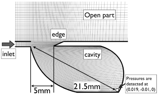
Figure 1: Geometry of the 2D ocarina. There are no tone holes other than the aperture in the upper-left corner of the cavity. A jet is blown from the left duct. The area of the cavity region is $1.635$ cm².

We are interested in relation between the pitch of sound vibration and the jet velocity. The excitation of over-tone will be prohibited if the sound vibration in ocarina mainly originates from the Helmholtz resonance. Then, the pitch of fundamental only depends on the volume of the cavity but irrespective to its shape.

2.1 Frequency of Helmholtz resonance

The resonance frequency of our two-dimensional model is estimated. We approximate that the effective length $L$ of open end correction is in proportion to the length of aperture $l$ and the proportional constant is $\alpha$. Then the effective mass $m$ and the spring constant $K$ for Helmholtz resonator are given by

$$\begin{split}m&=\rho lL\cong\rho\alpha l^{2}\\ K&=\rho l^{2}c^{2}/s,\end{split}$$ (1)

where $\rho$, $c$, and $s$ are the density of the air, the sound velocity, and the size of the cavity, respectively.

The resonant frequency $f_{0}$ can be written as follows:

$$f_{0}=\frac{1}{2\pi}\sqrt{\frac{K}{m}}.$$ (2)

Thus, the frequency of the two-dimensional Helmholtz resonance is

$$f_{2D}\approx\frac{c}{2\pi\sqrt{\alpha s}}.$$ (3)

Next, let’s estimate the $f_{2D}$ for our 2D model. Parameters of the model are

$$\begin{split}s&=1.6351\times 10^{-4}\\ l&=5.0\times 10^{-3}\\ c&=340.\end{split}$$ (4)

By the use of the above parameters, the value of Eq. (3) is estimated to

$$f_{2D}\approx 4.232\times 10^{3}\times\alpha^{-\frac{1}{2}}.$$ (5)

2.2 Sounds generated in the 2D model

Figure 2: Pressure in 2D ocarina with blow velocities: (a) 20 m/s; (b) 30 m/s; (c) 40 m/s. The corresponding normalized spectrum is shown in (a’), (b’), and (c’).

Numerically obtained pressure values and their normalized spectrum are shown in Fig.2. While the oscillation is very small and unstable for the blown velocity $20$ m/s, the oscillations are sufficiently grown for velocities $30$ m/s and $40$ m/s. In the figures of the normalized spectrum, almost no higher harmonics are observed in (b’) and (c’). The single oscillation without harmonics is one of the properties of the Helmholtz resonance.

Figure 3: Peak frequencies of the 2D ocarina for various blow velocities. The first, second, third, and fourth peaks in each velocity are shown in filled circles ($\bullet$), open circles ($\circ$), small squares ($\square$), and crosses ($\times$), respectively.

The frequency for the most prominent peak in each Fourier transformed data of the pressure are shown in Fig.3. As the velocity becomes larger, the frequency slightly increases. This shows a broad resonance which is often observed in ocarina, and the frequency as the Helmholtz resonance is about $2.5\times 10^{3}$ Hz. It is very difficult to obtain only from theoretical considerations with analogies from those simple Helmholtz instruments found in textbooks[1]. If we use this resonant frequency $2.5\times 10^{3}$ Hz for the formula in Section 2.1, the effective value of the open end correction for this model is determined as $\alpha\approx 2.87$ which is large in comparison with $\alpha\approx 16/3\pi$ in three-dimension.

The open end correction can be affected by the blow velocity (jet) on the aperture. One of the reason for the disagreement is that this effect is not considered in the estimation Eq.(5).

3 Three dimensional ocarina

Three dimensional ocarina model investigated here is shown in Fig.4. The numbers of mesh points for numerical calculations are tabulated in Table 1. A flow is added from the inlet duct and emitted as a jet at a $5\times 5$ mm² aperture to hit an edge. An open-box with $100\times 50\times 100$ mm³ is introduced above the aperture. The boundary conditions are the same as the two-dimensional case. In this section, the velocity of the jet is fixed to 10 m/s.

Table 1: The number of mesh points in 2D and 3D models

	points	faces	cells
2D model	27,062	53,130	13,200
3D model	1,434,041	4,197,500	1,382,000

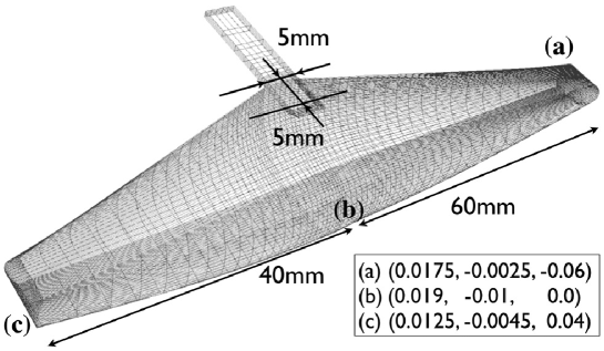
Figure 4: The whole geometry of the 3D ocarina model. In this figure, only thinned mesh points are shown. (a), (b), and (c) represent pressure observation points.

3.1 Frequency of Helmholtz resonance

The resonance frequency of a three dimensional Helmholtz resonator [1] is given by

$$f_{0}=\frac{1}{2\pi}\sqrt{\frac{K}{m}}=\frac{c}{2\pi}\sqrt{\frac{S}{VL}}$$ (6)

where $S$ is its aperture size and $V$ is volume of its cavity. In case of 3D, it is known that $L$ can be written as $L\cong 2\times 8a/3\pi$, where $a$ is the radius of the aperture. As in consequence, we get $f_{3D}$ as

$$f_{0}\approx\frac{c}{8}\sqrt{\frac{3\alpha}{V}}\approx\frac{c}{2\pi}\sqrt{\frac{1.85a}{V}}.$$ (7)

Next, let’s estimate $f_{3D}$ for our 3D model. Parameters of the model are

$$\begin{split}V&=9.425\times 10^{-6}\\ S&=2.5\times 10^{-5}\\ a&=2.82\times 10^{-3}\\ c&=340.\end{split}$$ (8)

Using these parameters, we can estimate the value of Eq. (7)

$$f_{3D}\approx 1.273\times 10^{3},$$ (9)

which should be compared to values obtained by numerical calculations.

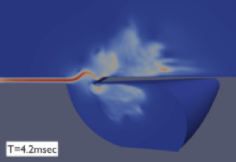
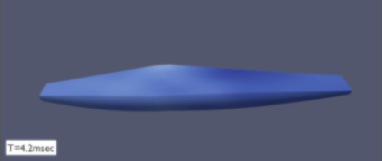
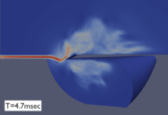
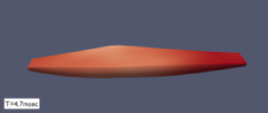
Figure 5: Internal fields in the 3D ocarina cavity: The left pictures represent snapshots of fluid velocity around an edge in the 3D ocarina model at $t=4.2$ msec and $t=4.7$ msec, which is shown by cutting at the center of the aperture; the right figures are distribution of pressure values in the cavity at $t=4.2$ msec and $t=4.7$ msec.

Figure 6: Oscillation observed in 3D ocarina driven by a 10 m/s jet: each figure shows pressure values detected in the three observation points (a), (b), and (c), respectively. The corresponding normalized spectrum is shown in (a’), (b’), and (c’).

3.2 Oscillation in ocarina

The fluid velocity around the edge and the pressure in the cavity obtained by the compressible LES solver (coodles in OpenFOAM v1.5) are shown in Fig.5, which are snapshots at $t=4.2$ msec and $t=4.7$ msec. Oscillations of sound pressure values detected at points (a), (b), and (c) in Fig.4 are shown in Fig.6 as well as Fourier transformed values. It is seen that the oscillation is synchronized over the whole cavity.

The frequency is determined as $8.8\times 10^{2}$ Hz from the Fourier transformation of the pressure data, This is lower than expected values from length resonances of the air-column, whose frequencies are obtained as $1.7\times 10^{2}$ Hz, $1.4\times 10^{2}$ Hz, and $2.1\times 10^{2}$ Hz from $10$ cm/$\frac{1}{2}\lambda$, $6$ cm/$\frac{1}{4}\lambda$, and $4$ cm/$\frac{1}{4}\lambda$, respectively. The expected frequency as the Helmholtz oscillator, Eq.(9), gives still larger than the frequency observed here. However, the theoretical calculation of Eq.(9) contains various uncertain factors on the open-end correction around the edge hole.

We have an actual ocarina instrument which was used to design the cavity for this calculation. The size of the ocarina is almost the same as the geometry given in this paper. According to an instruction of the ocarina, ’A₅’ (higher la) is the lowest note of this small instrument, i.e., the note when all the tone holes are closed. The frequency value of A₅ is assigned as 880 Hz in a usual musical scale. This is just the frequency observed. Thus, when we consider the frequency observed, we can conclude that our three dimensional model almost exactly reproduce the basic oscillation of the ocarina.

If we assume the basic mechanism in an ocarina as Helmholtz oscillation, it is expected that the internal oscillation of the cavity does not contain higher harmonics. However, the Fourier transformed spectrum in Fig.6 contains several peaks. This is mainly because the oscillation observed has not been grown sufficiently. Five milli-second used to analyze the oscillation is too short to observe stable oscillations in musical instruments. Moreover, a slightly higher blow velocity might be appropriate to drive the basic frequency. It is expected to clarify these points by executing more simulations with longer time.

4 Conclusion

In summary, we simulated an oscillation of a two and three dimensional ocarina by the use of the compressible LES solver in OpenFOAM 1.5. In both models, the resonance showed characteristic properties of the Helmholtz resonance. We conclude that the Helmholtz oscillation in a small air-reed instrument is properly reproduced by the compressible LES calculations.

As future works, various interesting investigations can be planned with the following theme: simulations of tone holes in which dynamic transitions between multiple frequencies; transitions between the Helmholtz resonance and the column-length resonance when we vary the geometry of the instrument; relation between the type of oscillations and sounding mechanisms [7].

References

- [1] N. H. Fletcher and T. D. Rossing, “The Physics of Musical Instruments,” Springer-Verlag, New York, 2nd edition (1998).
- [2] J. W. Coltman, “Sounding mechanism of the flute and organ pipe,” J. Acoust. Soc. Am. 44, 983–992 (1968).
- [3] T. Kobayashi, T. Takami, K. Takahashi, R. Mibu, and M. Aoyagi, “Sound Generation by a Turbulent Flow in Musical Instruments – Multiphysics Simulation Approach –,” in Proceedings of HPCAsia07, 91-96 (2007), arXiv:0709.0787v1 [physics.comp-ph]
- [4] C. Wagner, T. Hüttl, and P. Sagaut, ed. “Large-Eddy Simulation for Acoustics,” (Cambridge, 2007).
- [5] C. Seror, P. Sagaut, C. bailly, and D. Juvé, “On the radiated noise computed by large-eddy simulation,” Physics of Fluids, 13(2), 476-–487, 2001.
- [6] G. B. Brown, “The vortex motion causing edge tones,” Proc. Phys. Soc., London XLIX, 493–507 (1937).
- [7] M. J. Lighthill, “On sound generated aerodynamically,” Proc. R. Soc. London Ser. A 211, 564-–587 (1952).