Abstract

We compute one–loop corrections to the annihilation of non–relativistic particles $\chi$ due to the exchange of a (gauge or Higgs) boson $\varphi$ with mass $\mu$ in the initial state. In the limit $m_{\chi}\gg\mu$ this leads to the “Sommerfeld enhancement” of the annihilation cross section. However, here we are interested in the case $\mu\raisebox{-3.69899pt}{~{}\shortstack{$<$ \\ [-0.07cm] $\sim$}}~{}m_{\chi}$, where the one–loop corrections are well–behaved, but can still be sizable. We find simple and accurate expressions for annihilation from both $S-$ and $P-$wave initial states; they differ from each other if $\mu\neq 0$. In order to apply our results to the calculation of the relic density of Weakly Interacting Massive Particles (WIMPs), we describe how to compute the thermal average of the corrected cross sections. We apply this formalism to scalar and Dirac fermion singlet WIMPs, and show that the corrections are always very small in the former case, but can be very large in the latter. Moreover, in the context of the Minimal Supersymmetric Standard Model, these corrections can decrease the relic density of neutralinos by more than 1%, if the lightest neutralino is a strongly mixed state.

1 Introduction

The existence of non–baryonic Dark Matter (DM) in the universe is by now well established [1]. Recent observations determine the universal average DM density quite accurately. The exact value and its uncertainty depend somewhat on the assumptions made in the fit (“priors”). For example, within a minimal $\Lambda$CDM model, and combining data on the cosmic microwave background (CMB) anisotropies with observations of supernovae of type 1a and with analyses of baryon acoustic oscillations, one finds [2]:

$$\Omega_{\rm CDM}h^{2}=0.1131\pm 0.0034\,.$$ (1)

Here $\Omega_{\rm CDM}$ is the energy density of cold dark matter in units of the critical density, and $h$ is the scaled Hubble parameter such that $H_{0}=100\,h\,\mathrm{km}\,\mathrm{sec^{-1}}\,\mathrm{Mpc^{-1}}$ where $H_{0}$ is the current Hubble parameter. Introducing additional parameters in the fit can increase the allowed range; for example, significantly larger values of $\Omega_{\rm CDM}h^{2}$ are allowed if the number of particles that were relativistic when the CMB decoupled is kept free [2]. However, the minimal model describes the data well. Moreover, quite soon data from the Planck satellite are expected to reduce the error on $\Omega_{\rm CDM}h^{2}$ to the level of 1.5% using CMB measurements alone [3].

From the particle physics point of view, Weakly Interacting Massive Particle (WIMPs) are among the most attractive DM candidates. In standard cosmology their thermal relic density is naturally of the right order of magnitude. Owing to their weak interactions, they can be probed through both direct and indirect detection experiments [1], although no convincing signal has yet been found. Moreover, the existence of WIMPs is independently motivated in many extensions of the Standard Model (SM) of particle physics, the most prominent example being extensions based on supersymmetry (SUSY).

In order to fully exploit the precision of present cosmological data, the theoretical error on the prediction for the WIMP relic density should not exceed the error inferred from observations. For a given cosmological model, the WIMP relic density is determined uniquely by its annihilation cross section into SM particles, if all WIMPs were produced thermally. This requires that the post–inflationary Universe was sufficiently hot, with temperature exceeding about 5% of the WIMP mass. Moreover, one has to assume that no other, heavier particles decayed into WIMPs after WIMP decoupling. Under these conditions, which are satisfied for standard cosmology, the uncertainty of the current WIMP relic density is essentially given by the uncertainty of the WIMP annihilation cross section. In order to calculate this cross section to percent level accuracy, at least leading radiative corrections will have to be included.

In this paper we calculate one class of potentially sizable radiative corrections, which are due to the exchange of a boson between the WIMPs prior to their annihilation. If the mass $\mu$ of the exchanged boson vanishes, the one–loop expression diverges in the limit of vanishing relative velocity $v$ between the annihilating WIMPs. These large “Sommerfeld” corrections then have to be re–summed to all orders in the relevant coupling [4, 5, 6] (for earlier, related work see [7]). However, since WIMPs couple neither to photons nor to gluons, a new light boson with sizable coupling to the WIMPs, but not to SM particles, has to be introduced. The required hierarchy $\mu\ll m_{\chi}$, where $m_{\chi}$ is the mass of the WIMP, then raises naturalness issues.

Here we instead study the case $\mu\raisebox{-3.69899pt}{~{}\shortstack{$<$ \\ [-0.07cm] $\sim$}}~{}m_{\chi}$. Examples are the exchange of the light Higgs boson in the minimal supersymmetric extension of the SM (MSSM), and the exchange of the $Z$ boson in most “generic” WIMP models. If $\mu\raisebox{-3.69899pt}{~{}\shortstack{$<$ \\ [-0.07cm] $\sim$}}~{}m_{\chi}$ and $v\ll 1$ these corrections can be significantly bigger than the “generic” estimate $\alpha/\pi\sim$ (a few) $\times 10^{-3}$, while remaining small enough to permit simple one–loop calculations (and without threatening unitarity [8]). We calculate these corrections in the non–relativistic limit, following Iengo [5]. Since WIMPs decouple at temperature $T\simeq m_{\chi}/20$, an expansion in the relative velocity usually (but not always [9]) converges quite fast, and can therefore be used in the calculation of the one–loop correction. We also show how to compute the relevant thermal average over the corrected cross sections. We first apply our formalism to simple models with scalar or fermionic SM singlet WIMPs; the corrections are always small in the former case, but can be sizable in the latter scenario. We then analyze neutralino annihilation in the MSSM, and show that these corrections can reduce the relic density of strongly mixed neutralinos by more than 1%, comparable to the projected uncertainty of the value to be inferred from Planck data.

The rest of this paper is organized as follows. In Sec. 2 we introduce the formalism, which was initially proposed to treat non–perturbative Sommerfeld enhancement [5]. In particular, we factorize the correction to the amplitude due to the boson exchange between two incoming particles. In Sec. 3 we briefly review the standard calculation of dark matter relic density, and describe the thermal averaging of the corrected cross section. Numerical results for three WIMP models will be presented in Sec. 4. Finally we will summarize. Some details of our numerical procedure are described in Appendix A, while Appendix B shows that our approximate treatment indeed reproduces the leading terms of an exact calculation of radiative corrections associated with the initial state in a simple scalar model.

2 Correction to the annihilation amplitudes

Consider the annihilation of two WIMPs $\chi$ into two SM particles:

$$\chi(p_{1})+\chi(p_{2})\to X_{1}(p^{\prime}_{1})+X_{2}(p^{\prime}_{2})\,.$$ (2)

Generic tree–level diagrams contributing to this process have the form shown in Fig. 2. We want to compute one–loop corrections of the kind shown in Fig. 2, where a boson $\varphi$ is exchanged between the WIMPs before they annihilate, by adapting the formalism of Iengo [5, 10]. We assume that $\chi$ is a Majorana fermion; however, in the non–relativistic limit this will be relevant only for the case where the exchanged boson has axial vector couplings (see below).

In this formalism $\varphi$ exchange and $\chi$ annihilation are factorized; the former can then also be understood as re–scattering of the incoming WIMPs prior to their annihilation. This factorization ($\varphi$ exchange before $\chi$ annihilation) is only expected to work in the non–relativistic limit. Moreover, it requires the virtuality of the $\varphi$ propagator to be (much) smaller than that of the particle exchanged in $\chi$ annihilation. The latter can always be satisfied for $\mu\ll m_{\chi}$, where $\mu$ is the mass of the exchanged boson, but it can also be satisfied for $\mu\sim m_{\chi}$ if the WIMPs annihilate through the exchange of a particle $Y$ with mass $M_{Y}\gg m_{\chi}$. However, we will see that the corrections become small if $\mu\raisebox{-3.69899pt}{~{}\shortstack{$>$ \\ [-0.07cm] $\sim$}}~{}m_{\chi}$. Note also that these corrections do not capture UV effects like the renormalization of the tree–level couplings of $\chi$.

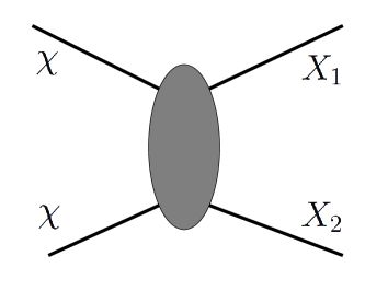
Figure 1: Tree–level WIMP annihilation. The grey blob represents the exchange of some particle in the $s-,\,t-$ or $u-$channel.

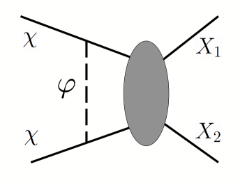
Figure 2: The one–loop corrections we are considering in this article. The meaning of the grey blob is the same as in Fig. 1.

Let $P=(p_{1}+p_{2})/2=(p^{\prime}_{1}+p^{\prime}_{2})/2$, $p=(p_{1}-p_{2})/2$ and $p^{\prime}=(p^{\prime}_{1}-p^{\prime}_{2})/2$; recall that $p_{1},\,p_{2}$ and $p^{\prime}_{1},\,p^{\prime}_{2}$ are the four–momenta in the initial and final state, respectively. In the cms we have $P_{0}=\sqrt{\vec{p}^{2}+m_{\chi}^{2}},\vec{P}=0$ and $p_{0}=0$. The initial state kinematics is thus fixed by $\vec{p}$. We write the one–loop corrected amplitude for annihilation from the partial wave denoted by $L$ as

$$A_{L}(|\vec{p}|,p^{\prime})=A_{0,L}(|\vec{p}|,p^{\prime})+\delta A_{L}(|\vec{p}|,p^{\prime})\,,$$ (3)

where $A_{0,L}$ and $\delta A_{L}$ denote the tree–level amplitude and the one–loop correction term, respectively. We are only interested in the cases $L=S$ and $L=P$. The contribution of higher partial waves is strongly suppressed during WIMP freeze–out.

The corrections can be calculated starting from the observation that annihilation from an $S-\ (P-)$wave initial state can be described by a pseudoscalar (scalar) $\chi$ current [11]. This allows to write the correction as a standard vertex (three–point function) correction. Let us begin with the simple case of scalar boson exchange:

$$\delta A_{L}(|\vec{p}|,p^{\prime}) = ig^{2}\bar{v}(p_{2})\int\frac{d^{4}q}{(2\pi)^{4}}\frac{\hbox to0.0pt{/\hss}q-\hbox to0.0pt{/\hss}P+m_{\chi}}{(q-P)^{2}-m_{\chi}^{2}+i\epsilon}\left(\gamma_{5}\right)^{n_{L}}\frac{\hbox to0.0pt{/\hss}q+\hbox to0.0pt{/\hss}P+m_{\chi}}{(q+P)^{2}-m_{\chi}^{2}+i\epsilon}$$ (4)

$$\hskip 71.13188pt\times\frac{1}{(p-q)^{2}-\mu^{2}+i\epsilon}\tilde{A}_{0,L}(|\vec{q}|,p^{\prime})\,u(p_{1})\,.$$

Here $g$ is the strength of the coupling between the boson and the WIMP, $n_{L}=1\ (0)$ for annihilation from an $S-\ (P-)$wave initial state, and the reduced tree-level amplitude $\tilde{A}_{0,L}$ describes the blob in Fig. 1 [except for the factor $\gamma_{5}$ in case of $S-$wave annihilation, which appears explicitly in Eq.(4)] as well as the final state. We will later show how to treat the exchange of spin–1 bosons.

As a first simplification, one then uses the fact that the full relativistic boson propagator satisfies $1/(k^{2}-\mu^{2})=-1/(\vec{k}^{2}+\mu^{2})\left[1-k_{0}^{2}/(k^{2}-\mu^{2})\right]$; the second term can be omitted in the non–relativistic limit, where the energy exchange is much smaller than the three–momentum exchange. Moreover, to leading order in the non–relativistic expansion, the $\vec{q}-$dependence of the reduced amplitude can be neglected, i.e. the factor $\tilde{A}_{0,L}$ can be pulled out of the integral. We then perform the integrals in Eq.(4) starting from the $q_{0}$ integration. We are looking for poles in the lower half–plane, with residues that diverge in the limit $\vec{q},\vec{p}\rightarrow 0$ [5]. This gives

$$\delta A_{L}(|\vec{p}|,p^{\prime})\simeq g^{2}\bar{v}(p_{2})\int\frac{d^{3}q}{(2\pi)^{3}}\frac{\left(\hbox to0.0pt{/\hss}q-\hbox to0.0pt{/\hss}P+m_{\chi}\right)\left(\gamma_{5}\right)^{n_{L}}\left(\hbox to0.0pt{/\hss}q+\hbox to0.0pt{/\hss}P+m_{\chi}\right)}{8\omega P_{0}\left(\omega-P_{0}\right)\left[\left(\vec{p}-\vec{q}\right)^{2}+\mu^{2}\right]}\tilde{A}_{0,L}(\vec{p}^{\prime})\,u(p_{1})\,,$$ (5)

where $\omega=\sqrt{\vec{q}^{2}+m_{\chi}^{2}}$; in the numerator one should take $q_{0}=\omega-P_{0}$. For small 3–momenta, we have

$$\omega-P_{0}\simeq\frac{\vec{q}^{2}-\vec{p}^{2}}{2m_{\chi}}\,;$$ (6)

note that this vanishes for $\vec{p},\vec{q}\rightarrow 0$, as advertised.

To zeroth order in the non–relativistic expansion we can set $\vec{q}\rightarrow 0$ in the numerator of Eq.(5). We see that this gives a non–vanishing result only if $n_{L}=1$, i.e. if a $\gamma_{5}$ matrix is present; recall that this corresponds to annihilation from an $S-$wave. To this order we can replace $\hbox to0.0pt{/\hss}P=P_{0}\gamma^{0}$ acting to the right (on the $u-$spinor) by $m_{\chi}$. The numerator of Eq.(5) then reduces to $4\gamma_{5}m_{\chi}^{2}$. Note that the factor of $\gamma_{5}$ is required in order to be able to access the large component of $\bar{v}(p_{2})$; this is most easily seen in the Dirac representation. Moreover, the factor $\omega P_{0}$ in the denominator of Eq.(5) can be replaced by $m_{\chi}^{2}$, up to corrections which are of second order in three–momenta.

To summarize, we have made three approximations:

1. We ignored the energy dependence of the $\varphi$ propagator.

2. In the $q_{0}$ integral we only kept the pole with the leading residue (in the non–relativistic limit).

3. We ignore all $\vec{q}$ dependence in the numerator (for annihilation from the $S-$wave).

Note that these approximations have to be taken simultaneously in order to get a UV–finite result. One may worry that this gives a rather poor approximation of the exact vertex correction even in cases where the latter are finite, as in a purely scalar theory. In Appendix B we show that this approximation can indeed differ substantially from the exact vertex correction if $\mu\ll m_{\chi}$. Note that the exact vertex correction by itself becomes IR–divergent for $\mu=0$. This leads to terms $\propto\log(m_{\chi}/\mu)$ which appear in the exact vertex correction, but not in our approximation. However, these terms are canceled by real emission diagrams and wave function corrections, which have to be included in order to obtain an IR–finite result for $\mu=0$. In Appendix B we show that, at least for a simple scalar model, our approximation does accurately reproduce the exact radiative correction associated with the initial state, whenever these corrections are large.

Let us therefore proceed with our calculation, which does not require additional approximations. The angular integrations are straightforward. One is then left with a single integral to describe the correction to $S-$wave annihilation:

$$\delta A_{S}(|\vec{p}|,p^{\prime})=\frac{g^{2}}{(2\pi)^{3}}\frac{\pi m_{\chi}}{|\vec{p}|}A_{0,S}\int^{\infty}_{0}d|\vec{q}|\frac{|\vec{q}|}{\vec{q}^{2}-\vec{p}^{2}}\ln{\frac{(|\vec{p}|+|\vec{q}|)^{2}+\mu^{2}}{(|\vec{p}|-|\vec{q}|)^{2}+\mu^{2}}}\,.$$ (7)

Note that we have absorbed the spinors into the full tree–level amplitude $A_{0,S}$. The one–loop correction to the cross section emerges from the interference between the correction $\delta A_{S}$ and the tree–level term $A_{0,S}$. We can thus write

$$\left.\delta A_{S}(|\vec{p}|,p^{\prime})\right|_{\rm 1-loop}=\frac{g^{2}}{4\pi^{2}}\frac{1}{v}A_{0}(|\vec{p}|,p^{\prime})I_{S}(r)\,,$$ (8)

where $v$ is the relative velocity between the two annihilating WIMPs in their center of mass frame (i.e., $|\vec{p}|=m_{\chi}v/2$), and we have defined the function

$$I_{S}(r)=\Re{\rm e}\left[\int_{0}^{\infty}dx\frac{x}{x^{2}-1}\ln{\frac{(1+x)^{2}+r}{(1-x)^{2}+r}}\right]\,.$$ (9)

Here $x=|\vec{q}|/|\vec{p}|$ and $r=\mu^{2}/\vec{p}^{2}$.

So far we have assumed that a spin–0 boson with scalar coupling is exchanged between the annihilating WIMPs. In order to treat more general cases, we rewrite the numerator of Eq.(5) as

$${\cal N}=\Gamma\left(\hbox to0.0pt{/\hss}q-\hbox to0.0pt{/\hss}P+m_{\chi}\right)\left(\gamma_{5}\right)^{n_{L}}\left(\hbox to0.0pt{/\hss}q+\hbox to0.0pt{/\hss}P+m_{\chi}\right)\bar{\Gamma}\,,$$ (10)

where $\Gamma$ describes the Dirac structure of the $\varphi\chi\chi$ coupling and $\bar{\Gamma}=\gamma^{0}\Gamma^{\dagger}\gamma^{0}$ its Dirac conjugate. Scalar exchange corresponds to $\Gamma=\bar{\Gamma}=1$.

It is easy to see that pseudoscalar exchange, $\Gamma=-\bar{\Gamma}=\gamma_{5}$, does not lead to enhanced contributions. For example, for $n_{L}=1$ and $q\rightarrow 0$ one finds a result $\propto\gamma_{5}\left(m_{\chi}-\hbox to0.0pt{/\hss}P\right)^{2}$, which is ${\cal O}(\vec{p}^{2})$.

Vector exchange corresponds to $\Gamma=\gamma^{\nu},\ \bar{\Gamma}=\gamma_{\nu}$, where the Lorentz index $\nu$ has to be summed. For $n_{L}=1$ and $q\rightarrow 0$ this gives

$${\cal N}_{\rm vector}=-2m_{\chi}\gamma_{5}\gamma^{\nu}\left(m_{\chi}+\hbox to0.0pt{/\hss}P\right)\gamma_{\nu}=-4m_{\chi}\gamma_{5}\left(2m_{\chi}-\hbox to0.0pt{/\hss}P\right)\,.$$

Again replacing $\hbox to0.0pt{/\hss}P$ by $m_{\chi}$ this leads to the same result as for scalar exchange, except for an overall sign. However, this sign is compensated by the extra minus sign in the vector boson propagator. We thus reproduce the well–known result that in the non–relativistic limit, the exchange of a vector boson has the same effect as that of a scalar boson.

Finally, axial vector exchange is described by setting $\Gamma=\gamma^{\nu}\gamma_{5},\ \bar{\Gamma}=\gamma_{\nu}\gamma_{5}$, where summation over $\nu$ is again implied. In the $S-$wave case, where $n_{L}=1$ and $q\rightarrow 0$ in the numerator, this gives

$${\cal N}_{\rm axial\ vector}=\gamma_{5}\gamma^{\nu}\left(\hbox to0.0pt{/\hss}P-m_{\chi}\right)^{2}\gamma_{\nu}=4m_{\chi}\gamma_{5}\left(2m_{\chi}+\hbox to0.0pt{/\hss}P\right)\,.$$

Again replacing $\hbox to0.0pt{/\hss}P$ by $m_{\chi}$, and accounting for the minus sign in the spin–1 propagator, we find that axial vector exchange differs from scalar or vector exchange by a factor of $-3$.

This does not seem to have been noticed in the recent literature. We therefore checked it in the limit where $\varphi$ exchange can be treated as re–scattering of the incoming WIMPs, leading again to two on–shell WIMPs. To leading order in velocity expansion we are interested in the limit of vanishing momentum exchange. However, we have to keep in mind that the two WIMPs will have to annihilate through a $\gamma_{5}$ vertex (for the $S-$wave case). This requires that the non–relativistic $u$ and $v$ spinors have the same spin. The rescattering process is then described by the quantity (we omit the bosonic propagator and all couplings)

$$A_{\rm res}=\sum_{s^{\prime}}\bar{v}(p_{2},s)\bar{\Gamma}v(p_{2},s^{\prime})\bar{u}(p_{1},s^{\prime})\Gamma u(p_{1},s)\,,$$ (11)

where $s,s^{\prime}$ describe the spin. Scalar boson exchange again corresponds to $\Gamma=\bar{\Gamma}=1$. In this case only $s^{\prime}=s$ contributes in the non–relativistic limit, where (in the cms) $p_{1}=p_{2}\simeq(m_{\chi},\vec{0})$, and one has $A_{\rm res,\ scalar}=-4m_{\chi}^{2}$. One immediately sees that pseudoscalar exchange only contributes at ${\cal O}(\vec{p}^{2})$.

In case of vector exchange, only $\Gamma=\gamma^{0}$ contributes to ${\cal O}(\vec{p}^{\,0})$ [5]. This then again requires $s=s^{\prime}$ in Eq.(11), giving $A_{\rm res,\ vector}=4m_{\chi}^{2}$. Remembering the additional minus sign in the spin–1 propagator we therefore again find that vector boson exchange contributes the same way as scalar exchange.

Finally, for axial vector exchange, only $\Gamma=\gamma_{i}\gamma_{5}\ (i=1,2,3)$ contribute to ${\cal O}(\vec{p}^{\,0})$. In this case $A_{\rm res}$ receives non–vanishing contributions both from $s=s^{\prime}$ and from $s=-s^{\prime}$, so that $A_{\rm res,\ axial\ vector}=-12m_{\chi}^{2}$. Again including the minus sign from the propagator, we reproduce our earlier result that axial vector exchange differs from scalar or vector exchange by a factor of $-3$. Note also that axial vector exchange describes an interaction between the spins of the two WIMPs. Such interactions are not suppressed at low velocities.

Now let us discuss $P-$wave annihilation, which corresponds to $n_{L}=0$ in Eq.(5). In this case setting $\vec{q}=0$ would lead to a result which is of ${\cal O}(\vec{p}^{2})$, i.e. of second order in the non–relativistic expansion. The leading term is the one linear in $\vec{q}$; the numerator of Eq.(5) then becomes $-4m_{\chi}\vec{q}\cdot\vec{\gamma}$. Note that the $\gamma_{i}$ again allow to access the large component of $\bar{v}(p_{2})$. The proper form of the correction term can then most easily be obtained using trace techniques, by dividing the 1–loop correction term $\delta A_{P}A_{0,P}^{\dagger}$ by the tree–level result $\left|A_{0,P}\right|^{2}$. We find that the $P-$wave correction term differs from the $S-$wave term by a factor $\vec{p}\cdot\vec{q}/\vec{p}^{2}$ inside the momentum integral. Performing the angular integrals, we can write this in the form of Eq.(8), with a new function describing the correction for annihilation from a $P-$wave initial state:

$$I_{P}=\Re{\rm e}\left\{\int_{0}^{\infty}dx\frac{2x^{2}}{x^{2}-1}\left[-1+\frac{x^{2}+1+r}{4x}\ln{\frac{(x+1)^{2}+r}{(x-1)^{2}+r}}\right]\right\}\,,$$ (12)

where $r=\mu^{2}/\vec{p}^{2}$ as above.

In order to treat the exchange of other bosons, non–trivial Dirac structures $\Gamma,\ \bar{\Gamma}$ again have to be introduced in Eq.(5), now for the case $n_{L}=0$. Proceeding as above, we find that pseudoscalar exchange does not lead to a large correction, while vector and axial vector exchange give the same correction as the exchange of a scalar boson. At first glance it may seem surprising that now axial vector exchange gives the same, positive, contribution; recall that in case of annihilation from an $S-$wave, axial vector exchange differed by a factor of $-3$. The difference can be understood from the observation that axial vector exchange leads to a spin–spin interaction of the form $4\vec{s}_{1}\cdot\vec{s}_{2}$, where $\vec{s}_{1,2}$ are the spins of the two WIMPs. This can be evaluated using $2\vec{s}_{1}\cdot\vec{s}_{2}=S^{2}-s_{1}^{2}-s_{2}^{2}$, where $\vec{S}=\vec{s}_{1}+\vec{s}_{2}$ is the total spin. In case of Majorana WIMPs, annihilation from an $S-$wave requires [11] $S=0$, leading to $4\vec{s}_{1}\cdot\vec{s}_{2}=-3$. For $P-$wave annihilation, we need [11] $S=1$, giving $4\vec{s}_{1}\cdot\vec{s}_{2}=1$. Note the relative factor of $-3$ between these two results.

At this point a comment on other WIMPs (than Majorana fermions) is in order. For a Dirac fermion–antifermion pair, there is no strict correspondence between the total spin and the orbital angular momentum. There will also be $S-$wave states with $S=1$ (as the $J/\psi$ family of quarkonia), as well as $P-$wave states with $S=0$. In this case the proper factor in front of the axial vector correction will depend on the spin state, i.e. it will no longer be completely process independent in this case. However, results for scalar, pseudoscalar and vector exchange are the same as for Majorana WIMPs. Finally, there is no such thing as an axial vector coupling to scalars, but our results for vector exchange apply to scalar WIMPs as well. Scalar exchange now involves a trilinear scalar interaction $f$, which has dimension of mass. Our results can describe this situation as well, with $g=f/(2m_{\chi})$.

The integrals in Eqs.(9) and (12) should be understood as principal value integrals, in order to treat the pole at $x=1$. In case $r\gg 1$ the integrals can be computed analytically, by expanding the logarithms in inverse powers of $r$. Moreover, in the limit $r\rightarrow 0$ both $I_{S}$ and $I_{P}$ approach $\pi^{2}/2$, thereby reproducing the well–known result [12] that the one–loop “Sommerfeld factor” for massless boson exchange is the same for $S-$ and $P-$partial waves. We also found accurate numerical expressions for small and moderate $r$. Altogether, the correction factors can be described by

$$I_{S}(r)\simeq\left\{\begin{array}[]{ll}\frac{2\pi}{\sqrt{r+1}}\left(1-\frac{1}{r+2}\right)&({\rm large}\ r)\\ \frac{\pi^{2}/2}{1+\frac{\sqrt{r}}{\pi}+\frac{r}{\pi^{2}}}&({\rm small}\ r)\end{array}\right.$$ (15)

$$I_{P}(r)\simeq\left\{\begin{array}[]{ll}\frac{2\pi}{3\sqrt{r+1}}\left(1+\frac{1.3}{r+1}\right)&({\rm large}\ r)\\ \frac{\pi^{2}/2}{1+\frac{3\sqrt{r}}{\pi}+\frac{r}{\pi}}&({\rm small}\ r)\end{array}\right.$$ (18)

The approximations for large and small $r$ intersect at $r\simeq 5.6\ (4.2)$ for $I_{S}\ (I_{P})$; the two approximations for $I_{P}$ intersect a second time at $r\simeq 6.3$.

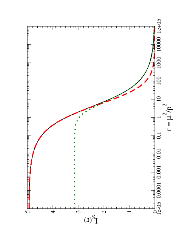
Figure 3: Comparison between the exact $I_{S}$ (solid, black) and its approximations for large $r$ (dotted, green) and small $r$ (dashed, red).

In Fig. 3, the exact function $I_{S}$ and its approximations are shown. By switching from the low$-r$ to the high$-r$ expression at the intersection point one reproduces the exact numerical result to better than 4% for all values of $r$. In case of $I_{P}$ (not shown) the large$-r$ approximation overshoots rather than undershoots the exact result for $10^{-3}\raisebox{-3.69899pt}{~{}\shortstack{$<$ \\ [-0.07cm] $\sim$}}~{}r\raisebox{-3.69899pt}{~{}\shortstack{$<$ \\ [-0.07cm] $\sim$}}~{}1$. This leads to slightly larger discrepancies, of up to 6%, between the exact $I_{P}$ and its approximations at $r\sim 5$ where the two approximations intersect. For the purpose of calculating the WIMP relic density a relative error on the correction of 6% is quite acceptable.

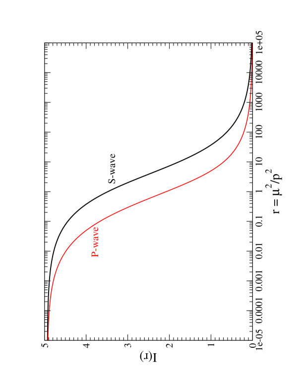
Figure 4: Comparison between $I_{S}$ describing the correction for annihilation from an $S-$wave (black) and $I_{P}$ describing the correction for annihilation from a $P-$wave (red or grey).

In Fig. 4 we show $I_{S}(r)$ and $I_{P}(r)$ as black and red (grey) lines, respectively. As noted earlier, the two functions coincide for massless exchange bosons, $r=0$. For nonvanishing boson mass, $r>0$, the $S-$wave contribution is larger than the $P-$wave one, by up to a factor of 3 at large $r$; see Eqs.(15). Note that for any finite mass of the exchanged boson, $\mu\neq 0$, the zero–velocity limit $|\vec{p}|\rightarrow 0$ corresponds to $r\rightarrow\infty$. Eqs.(15) show that asymptotically $I_{S,P}(r\rightarrow\infty)\propto 1/\sqrt{r}=|\vec{p}|/\mu$. Eq.(8) then shows that the corrections approach constant values of order $g^{2}m_{\chi}/(4\pi\mu)$ for $|\vec{p}|\rightarrow 0$, if $\mu\neq 0$. Such corrections will threaten the convergence of perturbation theory only if the WIMP and boson masses differ by a loop factor; in the technically more natural case where the boson mass lies a factor of a few below that of the WIMP, we still find a significant enhancement relative to the naive expectation that corrections should be of order $g^{2}/(16\pi^{2})$. We finally note that our numerical results are consistent with those in Ref. [6].

3 Dark Matter relic density

In this section we describe how to calculate the loop–corrected WIMP relic density from the loop–corrected WIMP annihilation cross section.

The evolution of the WIMP number density $n_{\chi}$ with time $t$ in the early Universe is governed by the Boltzmann equation [13]

$$\frac{dn_{\chi}}{dt}+3Hn_{\chi}=-\langle\sigma v\rangle\left(n_{\chi}^{2}-n_{\chi,{\rm eq}}^{2}\right)\,.$$ (19)

Here $H$ is the Hubble parameter describing the expansion of the Universe, $\sigma$ is the total WIMP annihilation cross section, $v$ is again the relative velocity between the annihilating WIMPs in their center of mass frame, $n_{\chi,{\rm eq}}$ is the WIMP number density in thermal equilibrium, and $\langle\dots\rangle$ denotes thermal averaging. For non–relativistic kinematics, the latter is given by

$$\langle\sigma v\rangle=\frac{2x^{3/2}}{\sqrt{\pi}}\int_{0}^{\infty}(\sigma v)\frac{v^{2}}{4}e^{-xv^{2}/4}dv\,,$$ (20)

where $x=m_{\chi}/T$, $T$ being the temperature of the thermal bath.

As long as the WIMP annihilation (or creation) rate is larger than the Hubble expansion rate, the WIMPs are (almost) in thermal equilibrium. However, once the annihilation rate falls below the expansion rate, WIMPs nearly decouple. Their present relic density is then to very good approximation given by [13]

$$\Omega_{\chi}h^{2}=\frac{8.5\times 10^{-11}~{}x_{F}~{}{\rm GeV}^{-2}}{\sqrt{g_{*}(x_{F})}J(x_{F})}\,.$$ (21)

Here $x_{F}=m_{\chi}/T_{F}$, where $T_{F}$ is the freeze–out temperature of the WIMPs, $g_{*}$ is the number of relativistic degrees of freedom, and the annihilation integral $J(x_{F})$ is defined as [13]

$$J(x_{F})=\int_{x_{F}}^{\infty}\!\!dx\frac{\langle\sigma v\rangle}{x^{2}}\,.$$ (22)

The freeze–out temperature of typical WIMPs is rather small, $T_{F}\simeq m_{\chi}/20$, hence WIMPs are non–relativistic when they freeze out. This suggests an expansion of $\sigma_{0}v$ in powers $v$ [13]:

$$\sigma_{0}v\simeq\mathscr{A}+\mathscr{B}v^{2}+\cdots\,,$$ (23)

where $\mathscr{A}$ and $\mathscr{B}$ are independent of $v$. Note that $\mathscr{A}$ contains only $S-$wave contributions, while $\mathscr{B}$ contains both $S-$ and $P-$wave contributions. While this often [9] works rather well for the tree–level cross section $\sigma_{0}$, the loop corrections we computed in the previous Section cannot be parameterized in this way. We saw in Fig. 4 that the correction factors $I_{S}$ and $I_{P}$ depend strongly on $v$ via the quantity $\sqrt{r}=\mu/|\vec{p}|=2\mu/(m_{\chi}v)$. We thus have to re–compute $\langle\sigma v\rangle$, which can then be used in Eq.(22) to derive the Dark Matter relic density using Eq.(21).

The 1–loop corrected WIMP annihilation cross section for partial wave labeled by $L$ can be written as

$$\sigma_{L}=\sigma_{0,L}+\delta\sigma_{L}\,.$$ (24)

Eq.(8) and the analogous expression for annihilation from the $P-$wave imply that

$$\delta\sigma_{S} = \frac{g^{2}}{2\pi^{2}v}I_{S}(r)\sigma_{0,S}\,;$$

$$\delta\sigma_{P} = \frac{g^{2}}{2\pi^{2}v}I_{P}(r)\sigma_{0,P}\,.$$ (25)

The thermal average over the tree–level cross section, expanded according to Eq.(23), can be computed easily [13]:

$$\langle\sigma_{0}v\rangle(x)\simeq\mathscr{A}+\frac{6\mathscr{B}}{x}\,.$$ (26)

In order to calculate the thermal averages over the correction terms, we rewrite the integral in Eq.(20) in terms of the integration variable $t=v\sqrt{x}$:

$$\langle\delta\sigma_{L}v\rangle=\frac{1}{2\sqrt{\pi}}\int_{0}^{\infty}dt\,t^{2}(\delta\sigma_{L}v){\rm e}^{-t^{2}/4}\,.$$ (27)

Eqs.(3) imply that the $t-$dependence of $\delta\sigma_{L}v$ takes the form $v^{n}I_{L}(r)=(t/\sqrt{x})^{n}I_{L}\left(\frac{4\mu^{2}x}{m_{\chi}^{2}t^{2}}\right)$, with $n=-1\ (+1)$ for annihilation from an $S-\ (P-)$wave initial state. This implies that the thermal average over the correction terms to the WIMP annihilation cross section can be written as $x^{-n/2}$ times a function of $z=2\mu\sqrt{x}/m_{\chi}$.

In Appendix A we describe how we parameterize the resulting functions for $S-$ and $P-$wave annihilation. The one–loop corrections to the “annihilation integrals” can then be written as

$$\delta J_{S}(x_{f}) = \frac{g^{2}\mathscr{A}}{\pi^{5/2}}\frac{\mu}{m_{\chi}}\int_{z_{F}}^{\infty}\frac{dz}{z^{2}}\left(\frac{1}{a_{S}z^{2}+b_{S}z+c_{S}}+d_{S}\right)\,,$$

$$\newline \delta J_{P}(x_{f}) = \frac{64g^{2}\mathscr{B}}{\pi^{5/2}}\left(\frac{\mu}{m_{\chi}}\right)^{3}\int_{z_{F}}^{\infty}\frac{dz}{z^{4}}\left[\exp(-a_{P}z+b_{P})+\frac{1}{c_{P}z+d_{P}}\right]\,.$$ (28)

Here $z_{F}=(2\mu/m_{\chi})\sqrt{x_{F}}$, and the coefficients $a_{S},\,b_{S},\,c_{S},\,d_{S}$ and $a_{P},\,b_{P},\,c_{P},\,d_{P}$ are given in Eqs.(38) and (44), respectively. We have made the simplifying assumption that $\mathscr{B}$ is dominated by $P-$wave contributions. This is true whenever the contribution $\propto\mathscr{B}$ to the annihilation integral is comparable to, or dominates over, the one $\propto\mathscr{A}$. In the opposite case the correction to the $\mathscr{B}-$term will in any case be insignificant.

Not surprisingly, the corrections are quadratic in the coupling of the exchanged boson to the WIMP. Moreover, they depend on the boson mass only through the ratio $\mu/m_{\chi}$. Recall finally that $I_{S}$ has to be multiplied with $-3$ if the exchanged boson has axial vector couplings; the same factor has to be included in $\delta J_{S}(x_{F})$.

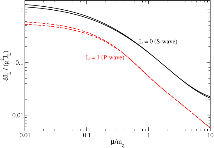
Figure 5: Corrections to the annihilation integrals for annihilation from the $S-$ wave (solid, black) and $P-$wave (dashed, red or grey), normalized to the tree–level results, and divided by the square of the WIMP coupling to the exchanged boson $g$. The upper (lower) curves are for inverse scaled freeze–out temperature $x_{F}=m_{\chi}/T_{F}=25\ (20)$.

In Fig. 5 we show the relative size of the loop corrections to the annihilation integrals for $S-$ and $P-$wave annihilation, divided by the square of the WIMP–boson coupling $g$. Eq.(21) shows that this also gives the relative change of the relic density due to our loop corrections, as long as the corrections are small, in which case $x_{F}$ remains essentially unchanged by these corrections; note that $x_{F}$ depends only logarithmically on the annihilation cross section. This is the main model–independent result of our paper. The size of the corrections to the relic density can be read off directly, by simply inserting the values of masses $\mu$ and $m_{\chi}$ and coupling $g$ given in a concrete model.

We see that the corrections are less important for $P-$wave annihilation. This is true even for $\mu\ll m_{\chi}$, where the loop functions $I_{S}$ and $I_{P}$ become equal. In this limit $v\delta\sigma_{S}\propto 1/v$ while $v\delta\sigma_{P}\propto v$. Performing the integrals for the thermal averaging, Eq.(20), and inserting the results into the definition of the annihilation integral, Eq.(22), one finds

$$\frac{\delta J_{P}/J_{P}}{\delta J_{S}/J_{S}}=\frac{4}{9}\ \ \ {\rm for}\ \mu\rightarrow 0\,.$$ (29)

The ratio becomes even smaller for nonvanishing $\mu$, because then $I_{P}<I_{S}$.

Fig. 5 shows results for $x_{F}=25$ (upper curves) and $x_{F}=20$ (lower curves); this spans the range of decoupling temperatures in usual WIMP models. One can easily show analytically that in the limit $\mu\rightarrow 0$, $\delta J_{L}/J_{L}\propto\sqrt{x_{F}}$ for both $L=0$ ($S-$wave) [14] and $L=1$ ($P-$wave). On the other hand, Fig. 5 shows that the relative correction to the annihilation integral becomes independent of $x_{F}$ once $\mu\raisebox{-3.69899pt}{~{}\shortstack{$>$ \\ [-0.07cm] $\sim$}}~{}0.3m_{\chi}$. This figure also shows that for the most plausible scenarios with electroweak strength couplings, possibly suppressed by mixing effects, where $g^{2}\raisebox{-3.69899pt}{~{}\shortstack{$<$ \\ [-0.07cm] $\sim$}}~{}0.5$, the loop corrections are significant only for $\mu\raisebox{-3.69899pt}{~{}\shortstack{$<$ \\ [-0.07cm] $\sim$}}~{}m_{\chi}$, as stated in the beginning of Sec. 2.

Two comments are in order before concluding this Section. First, Fig. 5 seems to imply that, especially for $P-$wave annihilation, the corrections are never very large. This is misleading. A simple one–loop calculation can be trusted only if $\delta\sigma<\sigma$ for all relevant velocities $v$. This requires $g^{2}I_{S,P}/(v\pi^{2})<1$. For $\mu\rightarrow 0$ this will always be violated at sufficiently small $v$, requiring summation of higher orders. In the standard treatment [4, 5, 6] this leads to $\delta\sigma\propto 1/v$ even for annihilation from a $P-$wave initial state. We saw at the end of Sec. 2 that for finite $\mu$ the maximal size of the correction to the cross section is of relative size $g^{2}m_{\chi}/(4\pi\mu)$. Our one–loop calculation can be trusted as long as this quantity is well below 1.

Secondly, it has very recently been pointed out [15] that Eq.(22) becomes inadequate for very small $\mu$. In this case the annihilation integral receives sizable contributions from quite large $x$, i.e. from low temperatures. Eq.(22) assumes that the WIMPs are in kinetic equilibrium while they are annihilating. It has to be modified for temperatures below the kinetic decoupling temperature, which is typically a few (tens of) MeV [16]. This modification can have sizable effects for very small $\mu$ [15]. However, we just saw that our strictly perturbative treatment is not reliable in this case anyway. Recall that $v\delta\sigma$ becomes constant, rather than scaling like $1/v$, for velocities below $v_{\rm crit}=\mu/m_{\chi}$. Our perturbative treatment will be reliable only if $\mu/m_{\chi}\gg g^{2}/(4\pi)\sim 0.01$. This implies that WIMP annihilation will quickly become irrelevant for $x>1/v^{2}_{\rm crit}\sim 10^{4}$, well before kinetic decoupling occurs.

4 Applications

In this Section we apply our results to existing WIMP models. We start with two simple models with scalar or fermionic SM singlets; in the third Subsection we discuss the more widely studied case of the MSSM neutralino.

4.1 Scalar singlet WIMP

This is the simplest WIMP model [17]. One only needs to introduce a single real scalar field $\chi$ to describe Dark Matter. If one forbids terms linear in $\chi$ by some (possibly discrete) symmetry in order to prevent $\chi$ decays, the only renormalizable coupling to SM fields allowed by all symmetries is of the form $\chi^{2}|h|^{2}$, where $h$ is the scalar Higgs doublet. Upon weak symmetry breaking this gives rise to a trilinear scalar interaction of the form $V\chi^{2}\phi$, where $\phi$ is the physical Higgs scalar of the SM and $V=246$ GeV the vacuum expectation value (vev) of the Higgs.

These interactions allow $\chi$ to annihilate via $\phi$ exchange in the $s-$channel; annihilation into two $\phi$ bosons is also allowed for $m_{\chi}>m_{\phi}$. An accurate tree–level calculation of the resulting relic density has been performed in [18]. Writing the coefficient of the $\chi^{2}|h|^{2}$ term in the Lagrangian as $-k/2$, they find that the correct relic density (1) is obtained for $k\simeq 0.28m_{\chi}/(1\ {\rm TeV})$, unless $m_{\chi}\sim m_{\phi}/2$, in which case an even smaller $k$ is required. We can use our formalism to compute corrections to this result from $\phi$ exchange prior to annihilation, i.e. $\varphi=\phi$ in this case. This gives a coupling factor $k^{2}V^{2}/(4m_{\chi}^{2})\simeq 0.0012$, (almost) independent of $m_{\chi}$. Fig. 5 shows that the corrections due to $\phi$ exchange in the initial state will then at best be at the permille level. In this model we therefore do not find any significant radiative corrections involving the initial state only. This should also hold for the inert doublet model [19], since the coupling between the inert WIMP doublet and the SM Higgs boson will have to satisfy a similar relation.

4.2 Fermionic singlet WIMP

The next simplest WIMP model [20] contains a Dirac fermion SM singlet $\chi$ as well as a real scalar singlet $\varphi$, with couplings $g\bar{\chi}\chi\varphi+A\varphi|h|^{2}$, where $h$ is again the Higgs doublet of the SM. The latter term induces mixing between the singlet $\varphi$ and the SM Higgs boson, allowing $\varphi$ to decay. If this mixing is small and $m_{\varphi}<m_{\chi}$, the dominant $\bar{\chi}\chi$ annihilation channel is into two $\varphi$ bosons, via $t-$ and $u-$channel diagrams. In the non–relativistic limit this is a pure $P-$wave process, with tree–level cross section

$$v\sigma(\bar{\chi}\chi\rightarrow\varphi\varphi)=\frac{g^{4}v^{2}\beta}{24\pi}\frac{m_{\chi}^{2}\left(9m_{\chi}^{4}-8m_{\chi}^{2}m_{\varphi}^{2}+2m_{\varphi}^{4}\right)}{\left(2m_{\chi}^{2}-m_{\varphi}^{2}\right)^{4}}+{\cal O}(v^{4})\,,$$ (30)

where $\beta=\sqrt{1-m_{\varphi}^{2}/m_{\chi}^{2}}$. In the limit $m_{\chi}^{2}\gg m_{\varphi}^{2}$ this simplifies to

$$v\sigma(\bar{\chi}\chi\rightarrow\varphi\varphi)=\frac{3g^{4}v^{2}}{128\pi m_{\chi}^{2}}\,.$$

The tree–level calculation therefore predicts the correct relic density (1) for coupling

$$g^{2}\simeq 0.2\frac{m_{\chi}}{100\ {\rm GeV}}\,.$$

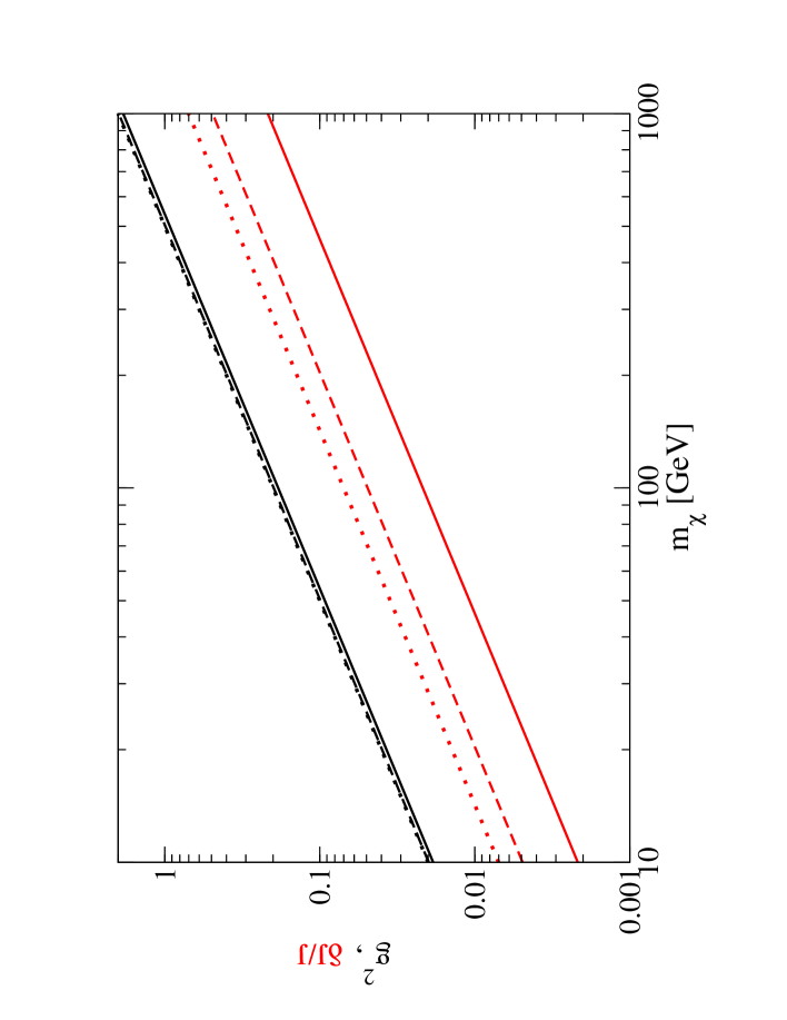
Figure 6: Strength of the $\bar{\chi}\chi\varphi$ coupling $g$ (black), as well as the resulting one–loop correction to the annihilation integral (red), in a model with Dirac fermion singlet DM. $g$ has been computed from the requirement that $\bar{\chi}\chi\rightarrow\varphi\varphi$ annihilation produces the correct $\chi$ relic density at tree level. The solid (dashed, dotted) curves are for $\mu/m_{\chi}=0.5\ (0.2,\ 0.1)$, where $\mu\equiv m_{\varphi}$.

This can then be used to read off the correction due to $\varphi$ exchange in the initial state from Fig. 5, with $\mu=m_{\varphi}$. The result is shown in Fig. 6, where we have used the exact (tree–level) result (30) to derive the required coupling strength. The black curves show that this coupling strength depends only very weakly on the mass of the scalar for $\mu\equiv m_{\varphi}\raisebox{-3.69899pt}{~{}\shortstack{$<$ \\ [-0.07cm] $\sim$}}~{}0.5m_{\chi}$. Note that the cross section slightly increases with increasing $m_{\varphi}$ as long as $m_{\varphi}<0.85m_{\chi}$. The reason is that increasing $m_{\varphi}$ allows the $t-$ and $u-$channel propagators to be less off–shell, as shown by the denominator in Eq.(30). As a result, the required coupling strength slightly decreases with increasing $m_{\varphi}$.

However, the red curves show that this effect is much smaller than the strong dependence of $\delta J_{P}/J_{P}$ on $\mu/m_{\chi}$ illustrated in Fig. 5. More importantly, we see that the corrections due to $\varphi$ exchange in the initial state can easily exceed the uncertainty of the observational determination of the DM relic density; for $\mu/m_{\chi}=0.5\ (0.2,\ 0.1)$ they even reach the 10% level for $m_{\chi}>450\ (210,\ 130)$ GeV. Since the correction is positive, one would have to reduce the coupling in order to obtain the correct relic density after inclusion of one–loop corrections. This would correspondingly reduce all interactions between the WIMP $\chi$ and the SM particles, all of which are mediated by $\varphi$ exchange.

4.3 The lightest neutralino in the MSSM

We finally want to apply our formalism to the lightest neutralino in the minimal supersymmetric extension of the Standard Model (MSSM), which is the probably best motivated WIMP, and certainly the most widely studied [1, 21] one. For simplicity we will assume that sfermions are heavy. Given experimental lower bounds on the masses of sfermions and Higgs bosons, relatively light sfermions by themselves typically only lead to an acceptable neutralino relic density in the presence of significant co–annihilation [22]. This involves several particles, with mass splittings of order of the absolute value of the 3–momentum in the initial state. These more complicated scenarios cannot be treated with the formalism presented in this paper.

Generally speaking, in the MSSM the neutralinos are mixtures of the $U(1)_{Y}$ gaugino $\tilde{B}$, the neutral $SU(2)$ gaugino $\widetilde{W}_{3}$, and of the two neutral higgsinos $\tilde{h}_{1}^{0},\ \tilde{h}_{2}^{0}$:

$$\tilde{\chi}^{0}_{i}=N_{i1}\tilde{B}+N_{i2}\widetilde{W}_{3}+N_{i3}\tilde{h}_{1}^{0}+N_{i4}\tilde{h}_{2}^{0}\,\ (i=1,\cdots,4).$$ (31)

The coefficients $N_{ik}$ satisfy the sum rule $\sum_{k=1}^{4}\left|N_{ik}\right|^{2}=1\ \forall i$. Most phenomenological analyses of the MSSM assume that the soft SUSY breaking gaugino masses unify at or near the scale of Grand Unification [21]. This implies that the $U(1)_{Y}$ gaugino mass is about half the $SU(2)$ gaugino mass near the TeV scale. As a result, the Wino component of our candidate WIMP, the lightest neutralino ($\chi\equiv\tilde{\chi}_{1}^{0}$), is subdominant, i.e. $\left|N_{11}\right|^{2}\gg\left|N_{12}\right|^{2}$. If sfermions are heavy, $\chi$ annihilation involves couplings of the lightest neutralino to gauge or Higgs bosons, which vanish in the pure Bino limit ($\left|N_{11}\right|\rightarrow 1$). In models with gaugino mass unification and heavy sfermions, the annihilation cross section can thus only be sufficiently large if $\chi$ has significant higgsino components.

On the other hand, for a nearly pure higgsino, where $\left|N_{11}\right|^{2}+\left|N_{12}\right|^{2}\ll 1$, the cross section for annihilation into $W^{+}W^{-}$ and $Z^{0}Z^{0}$ pairs is so large that a mass $m_{\chi}\simeq 1$ TeV is required to obtain the correct relic density (1) [24]. Such a large mass for the lightest superparticle is at odds with the primary motivation for postulating the existence of superparticles, which is the stabilization of the weak scale against quadratically divergent quantum corrections.

Assuming gaugino mass unification, the most natural neutralino satisfying the constraint (1) is therefore a bino–higgsino mixture, dubbed a “well–tempered neutralino” in ref.[25]. Note that the neutralino couplings to Higgs bosons involves products of a combination of gaugino components ($N_{i2}-\tan\theta_{W}N_{i1}$, where $\theta_{W}$ is the weak mixing angle) with one of the higgsino components ($N_{i3},\ N_{i4}$). These couplings are maximal in the region of strong gaugino–higgsino mixing, and should thus be sizable for the “well–tempered” neutralino. Moreover, as well known, at least one of the neutral MSSM Higgs bosons is rather light, with mass below 130 GeV. This leads one to expect potentially sizable 1–loop corrections due to the exchange of a Higgs boson prior to WIMP annihilation.

We checked this with the help of the the code micrOMEGAs 2.2 [26]. Among other things, this program computes the complete tree–level neutralino annihilation cross sections for all two–body final states. It does not resort to the non–relativistic expansion (23), but one can easily determine the coefficients $\mathscr{A}$ and $\mathscr{B}$ by calculating the annihilation cross section at two different values of $v$, i.e. for two (slightly) different cms energies $\sqrt{s}$. These coefficients are then used in Eqs.(3) to compute the corrections to the annihilation integral; we emphasize that we continue to use the full cross sections, not their non–relativistic expansions, for the calculation of the tree–level contribution to the annihilation integral. We also take $x_{F}$ from the program. The one–loop corrected $\chi$ relic density can then be expressed as

$$\Omega_{\chi}h^{2}=\Omega_{\chi,0}h^{2}\frac{J_{0}(x_{F})}{J_{0}(x_{F})+\delta J(x_{F})}\,$$ (32)

where $\delta J=\delta J_{S}+\delta J_{P}$, and the tree–level value $J_{0}(x_{F})$ can be calculated from the program’s tree–level prediction $\Omega_{\chi,0}h^{2}$ using Eq.(21).

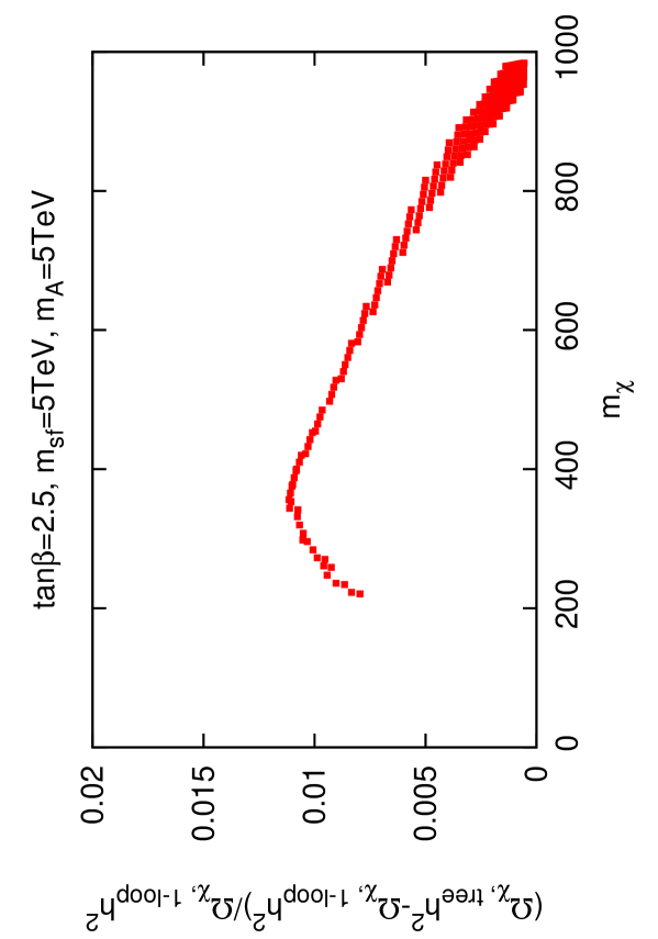
Figure 7: The relative size of one-loop correction to the relic density of a “well-tempered” neutralino. The ratio between $M_{1}$ and $\mu$ is fixed such that the relic density satisfies the constraint (1) within two standard deviations. We take $M_{2}=2M_{1}$, consistent with gaugino mass unification, $\tan\beta=2.5$, and assume sfermions and most Higgs bosons to be very heavy. Scenarios with $m_{\chi}<200$ GeV are excluded by Higgs boson searches.

The result is shown in Fig. 7. It has been generated using micrOMEGAs [26], using Softsusy [27] to calculate the superparticle and Higgs boson spectrum; we specify the input directly at the weak scale. All points satisfy the relic density constraint (1) within two standard deviations. For simplicity we take (unnaturally) large values for the masses of all sfermions and of the CP–odd Higgs boson $A$, but the results would not change significantly as long as $m_{\rm sf}\raisebox{-3.69899pt}{~{}\shortstack{$>$ \\ [-0.07cm] $\sim$}}~{}2m_{\chi}$ and $m_{A}\raisebox{-3.69899pt}{~{}\shortstack{$>$ \\ [-0.07cm] $\sim$}}~{}3m_{\chi}$. We include loop corrections due to exchange of the $Z-$boson as well as both CP–even neutral Higgs boson, but the contribution from the heavier Higgs boson is totally negligible due to its large mass.

We see that the corrections are most important for $m_{\chi}$ near 350 GeV. For smaller WIMP mass the corrections are reduced because the higgsino component of $\chi$ becomes smaller, and because the ratio of light Higgs and WIMP masses becomes smaller, which reduces the loop functions. The latter effect would tend to increase the correction for heavier WIMPs. However, for $m_{\chi}>350$ GeV the gaugino components of $\chi$ decrease quickly; this reduces its coupling to the light Higgs boson, which is most important here. Moreover, for $m_{\chi}\raisebox{-3.69899pt}{~{}\shortstack{$>$ \\ [-0.07cm] $\sim$}}~{}900$ GeV, co–annihilation with $\tilde{\chi}_{1}^{\pm}$ and $\tilde{\chi}_{2}^{0}$ become important [11, 28, 24]. The effect of light boson exchange corrections to co–annihilation is beyond the scope of our paper, and has not been included in Fig. 7. As a result, the correction becomes comparable to the anticipated post–PLANCK precision of the observational determination of $\Omega_{\chi}h^{2}$ only for a rather narrow range of $m_{\chi}\sim 350$ GeV. This is consistent with the results of Fig. 5, given the fact that the coupling of our “well–tempered” neutralino to the lightest Higgs boson does not exceed 0.2.

The small size of the corrections due to boson exchange in the initial state indicate that these may well not be the leading radiative corrections in the MSSM. In fact, full electroweak one–loop calculations [14, 29] found much larger corrections in some cases. These are presumably due to UV–sensitive effects, which cannot be treated using our formalism. Moreover, QCD corrections can significantly affect the annihilation cross section into quarks [14, 30].

5 Summary and Discussion

We have calculated one–loop corrections to the WIMP annihilation cross section, and the corresponding corrections to the relic density, due to the exchange of a relatively light boson between the WIMPs.

The formalism for calculating the corrections to the cross section is described in Sec. 2. We used a non–relativistic formalism [10, 5], i.e. we only included small loop momenta. The correction can then also be understood as re–scattering of the WIMPs prior to their annihilation. The motivation for this is that these configurations can give rise to sizable corrections if the exchanged boson is lighter than the WIMP and the relevant coupling is not too small. Note that these corrections are universal, i.e. they are the same for all final states. However, we saw that they do depend on the partial wave of the initial state, being smaller for annihilation from the $P-$wave if the exchanged boson is massive. The main result of this Section is that these corrections can be described by loop functions which only depend on the ratio of the mass of the exchanged boson and the cms three–momentum of the annihilating WIMPs; simple yet accurate parameterizations for these loop functions are given in Eqs.(15). We also checked explicitly that the correction is independent of the form of the coupling of the exchanged boson, except for the case of axial vector exchange in the $S-$wave, where an additional factor of $-3$ is required. Moreover, the corrections can be used for scalar as well as fermionic WIMPs.

In Sec. 3 we computed the resulting correction to the relic density. We saw that the thermal averaging and the calculation of the “annihilation integral” further reduce the relative importance of the corrections in case of annihilation from a $P-$wave initial state. The main model–independent result of our paper is shown in Fig. 5, which shows the relative size of the corrections to the annihilation integral – or, almost equivalently, to the relic density – as a function of the ratio of the masses of the exchanged boson and the WIMP. We saw that for ${\cal O}(1)$ coupling between boson and WIMP, the corrections are significant unless the boson is heavier than the WIMP.

Finally, in Sec. 4 we applied this formalism to several WIMP models. We showed that these corrections are very small for a scalar singlet WIMP, but can be very large for a Dirac fermion singlet WIMP annihilating into a light scalar singlet. Finally, we analyzed the “well–tempered” neutralino, which is a mixture of $U(1)_{Y}$ gaugino and higgsinos, and found corrections comparable to the anticipated post–PLANCK precision of the observationally determined WIMP relic density only for a narrow range of neutralino masses near 350 GeV. The main reason is that the relevant coupling is always below 0.2 in this case. In a supersymmetric scenario, bigger couplings of WIMPs to Higgs bosons are e.g. possible for “singlino” Dark Matter in scenarios where the MSSM is extended by an additional Higgs singlet superfield [31].

In the MSSM diagonal couplings of the lightest neutralino to gauge or Higgs bosons are always suppressed by mixing angles. Off–diagonal couplings may be large, however. These can give rise to sizable corrections if these couplings involve particles that are only slightly heavier than the lightest neutralino. Such states, with sizable couplings to the lightest neutralino, often exist in regions of parameter space where co–annihilation is important. In order to treat this, one has to extend the formalism presented here to scenarios where the particles in the loop have slightly different masses than the annihilating external particles. Moreover, if co–annihilation with a sfermion is important, there are vertex corrections involving the exchange of an SM fermion, rather than a boson, between the co–annihilating particles. This offers another avenue for future work.

Acknowledgment

We thank A. Pukhov for his help with using micrOMEGAs. KIN is supported in part by Grants-in-Aid for Scientific Research from the Ministry of Education, Culture, Sports, Science, and Technology of Japan, and by the Grant-in-Aid for Nagoya University Global COE Program, “Quest for Fundamental Principles in the Universe: from Particles to the Solar System and the Cosmos”, from the Ministry of Education, Culture, Sports, Science and Technology of Japan. MD and JMK are partially supported by the Marie Curie Training Research Networks “UniverseNet” under contract no. MRTN-CT-2006-035863, and “UniLHC” under contract no. PITN-GA-2009-237920.

Appendix A: Parameterizations of the thermal averages

The thermal average of the correction to the $S-$wave annihilation cross section is given by

$$\langle\delta\sigma_{S}v\rangle = \frac{x^{3/2}}{2\pi^{1/2}}\int_{0}^{\infty}v^{2}\left(\frac{g^{2}}{2\pi^{2}v}I_{S}(v)(\sigma_{0,S}v)\right){\rm e}^{-xv^{2}/4}$$ (33)

$$= \frac{g^{2}x^{3/2}}{4\pi^{5/2}}\cdot\mathscr{A}\cdot\int_{0}^{\infty}v^{2}\left(\frac{I_{S}(v)}{v}\right){\rm e}^{-xv^{2}/4}\,.$$

$\mathscr{A}$ has been defined via the nonrelativistic expansion of $\sigma v$ in Eq.(23). The $v-$dependence of $I_{S}$ can be read off Eq.(15):

$$I_{S}(v)\simeq\left\{\begin{array}[]{ll}\frac{2\pi v\sqrt{u^{2}+v^{2}}}{u^{2}+2v^{2}},&v\leq\frac{u}{2.4}\\ \frac{\pi^{2}/2}{1+\frac{u}{\pi v}+\frac{u^{2}}{\pi^{2}v^{2}}},&v>\frac{u}{2.4}\end{array}\right..$$ (36)

Here we have introduced the quantity $u=2\mu/m_{\chi}$. We showed in Sec. 3 that the integral in Eq.(33) is a function of the variable $z=u\sqrt{x}$. We find the following fitting function for the “thermally averaged” $(I_{S}/v)$, defined as the integral in the last line of Eq.(33):

$$\langle\frac{I_{S}}{v}\rangle_{\rm fit}=\frac{1}{x}\left(\frac{1}{a_{S}z^{2}+b_{S}z+c_{S}}+d_{S}\right),$$ (37)

with

$$a_{S}=0.000593;\ b_{S}=0.03417;\ c_{S}=0.1015;\ d_{S}=0.1182.$$ (38)

For the $P-$wave,

$$\langle\delta\sigma_{P}v\rangle = \frac{x^{3/2}}{2\pi^{1/2}}\int_{0}^{\infty}v^{2}\left(\frac{g^{2}}{2\pi^{2}v}I_{P}(v)(\sigma_{0,P}v)\right){\rm e}^{-xv^{2}/4}$$ (39)

$$= \frac{g^{2}x^{3/2}}{4\pi^{5/2}}\cdot\mathscr{B}\cdot\int_{0}^{\infty}v^{2}\left(v^{2}\cdot\frac{I_{P}(v)}{v}\right){\rm e}^{-xv^{2}/4},$$

with

$$I_{P}(v)\simeq\left\{\begin{array}[]{ll}\frac{2\pi v\left(u^{2}+2.3v^{2}\right)}{3(u^{2}+v^{2})^{3/2}},&v\leq\frac{u}{2.1}\\ \frac{\pi^{2}/2}{1+\frac{3u}{\pi v}+\frac{u^{2}}{\pi v^{2}}},&v>\frac{u}{2.1}\end{array}\right..$$ (42)

As above, we find a fitting function for the “thermally averaged” $(vI_{P})$:

$$\langle vI_{P}\rangle_{\rm fit}=\frac{16}{x^{2}}\left({\rm e}^{-a_{P}z-b_{P}}+\frac{1}{c_{P}z+d_{P}}\right),$$ (43)

with

$$a_{P}=0.318;\ b_{P}=0.1226;c_{P}=0.3309;d_{P}=0.6306.$$ (44)

Appendix B: Comparison to a full one–loop calculation

In this Appendix we compare our approximate treatment of corrections due to $\varphi$ exchange with a full one–loop calculation. We do this in the framework of a purely scalar theory, where the exact vertex correction is UV finite. As we remarked in Sec. 2, our formalism will not capture corrections associated with the renormalization of the coupling(s) relevant for WIMP annihilation, so chosing an example with UV–finite vertex correction greatly simplifies the comparison to the full one–loop calculation.

Figure 8: Feynman diagrams describing full initial state radiative corrections: vertex correction (a), wave function renormalization (b) and real emission (c); wave function renormalization of, and emission off, the upper leg also has to be included. The WIMP $\chi$ and the exchanged boson $\varphi$ are denoted by black and red (grey) dashed lines, respectively, while the blob denotes the $\chi\chi$ annihilation vertex, which is independent of the $\chi$ momenta.

The Feynman diagrams describing exact one–loop corrections associated with the initial state are shown in Fig. 8. Here the blob describes the (tree–level) $\chi$ annihilation process; this could e.g. be a quartic vertex involving two lighter scalars, or a trilinear vertex coupling to the $s-$channel propagator of another scalar particle. For the purpose of our calculation we only need to know that the rest of the diagram described by the blob is independent of the loop momentum. We describe the $\varphi\chi\chi$ vertex by the (dimensionful) coupling $\kappa$.

Let us begin by computing the vertex correction; recall that this is the only diagram that contributes in the approximate treatment of Sec. 2. It gives:

$$\frac{A_{\rm vertex}}{A_{0}}=i\kappa^{2}\int\frac{d^{4}q}{(2\pi)^{4}}\frac{1}{(P+q)^{2}-m^{2}_{\chi}}\frac{1}{(P-q)^{2}-m_{\chi}^{2}}\frac{1}{(p-q)^{2}-\mu^{2}}\,.$$ (45)

Here $A_{0}$ is the tree–level matrix element described by the blob in Fig. 8. Recall that $P=(p_{1}+p_{2})/2,\ p=(p_{1}-p_{2})/2$, where $p_{1,2}$ are the 4–momenta of the incoming WIMPs, $\mu$ is the mass of $\varphi$, and $\kappa$ is the $\chi\chi\varphi$ coupling.

The loop integral in Eq.(45) can be computed straightforwardly using Feynman parameters, giving

$$\frac{A_{\rm vertex}}{A_{0}}=-\frac{\kappa^{2}}{16\pi^{2}}C_{0}(s,m_{\chi}^{2},m_{\chi},m_{\chi},\mu^{2})\,.$$ (46)

Here $C_{0}$ is the scalar Passarino–Veltman three–point function in the convention of ref.[32].

The loop integral in Eq.(45) can also be evaluated directly, following the steps of Sec. 2 but without making any approximations in the propagators. We first perform the energy ($q_{0}$) integrals by contour integration, by summing over the residues of all poles in the lower half plane. In general, there are three such poles:

$$q_{0}^{\rm pole\ 1} = \omega-P_{0}\,;$$

$$q_{0}^{\rm pole\ 2} = \omega+P_{0}\,;$$

$$q_{0}^{\rm pole\ 3} = \sqrt{(\vec{p}-\vec{q})^{2}+\mu^{2}}\,,$$ (47)

where $\omega=\sqrt{\vec{q}^{2}+m_{\chi}^{2}}$ as in Eq.(5). Only the first pole has a residue that diverges in the limit $\vec{p},\vec{q}\rightarrow 0$. The third pole comes from the energy dependence of the $\varphi$ propagator, which has been ignored in the approximate treatment of Sec. 2. The angular integrals can also be performed straightforwardly. After some algebra, we arrive at:

$$\frac{A_{\rm vertex}}{A_{0}} = \frac{\kappa^{2}}{16\pi^{2}}\frac{1}{4P_{0}|\vec{p}|}\int_{0}^{\infty}|\vec{q}|d|\vec{q}|\left[\frac{1}{\omega(\omega-P_{0})}\ln\frac{\left(|\vec{p}|+|\vec{q}|\right)^{2}+\mu^{2}-\left(\omega-P_{0}\right)^{2}}{\left(|\vec{p}|-|\vec{q}|\right)^{2}+\mu^{2}-\left(\omega-P_{0}\right)^{2}}\right.$$

$$\hskip 105.27519pt\left.-\ \frac{1}{\omega(\omega+P_{0})}\ln\frac{\left(|\vec{p}|+|\vec{q}|\right)^{2}+\mu^{2}-\left(\omega+P_{0}\right)^{2}}{\left(|\vec{p}|-|\vec{q}|\right)^{2}+\mu^{2}-\left(\omega+P_{0}\right)^{2}}\right.$$

$$\hskip 105.27519pt\left.+\ \frac{1}{\omega_{\varphi}^{2}}\left(\ln\frac{\mu^{2}+2|\vec{p}||\vec{q}|-2P_{0}\omega_{\varphi}}{\mu^{2}-2|\vec{p}||\vec{q}|-2P_{0}\omega_{\varphi}}-\ln\frac{\mu^{2}+2|\vec{p}||\vec{q}|+2P_{0}\omega_{\varphi}}{\mu^{2}-2|\vec{p}||\vec{q}|+2P_{0}\omega_{\varphi}}\right)\right]\,.$$

In the last line, we have introduced $\omega_{\varphi}=\sqrt{\vec{q}^{2}+\mu^{2}}$.

It is easy to see that the first term reduces to our expression (7) if we use the non–relativistic expansion for $\omega$, which includes dropping the terms $(\omega-P_{0})^{2}$ in the argument of the logarithm. However, for large $|\vec{q}|$ these latter terms are important. They imply that the logarithm approaches the constant value $2|\vec{p}|/P_{0}$ in the limit $|\vec{q}|\rightarrow\infty$, rather than vanishing as in Eq.(7). As a result, the first line of the right–hand side (rhs) of Eq.(Appendix B: Comparison to a full one–loop calculation) by itself is logarithmically UV–divergent. The second line contributes the same UV divergence again; only after adding the contribution in the third line we obtain a UV–finite result. This third line comes from the third pole in Eq.(Appendix B: Comparison to a full one–loop calculation), which does not exist if one drops the energy dependence of the $\varphi$ propagator, as in Sec. 2. This proves our statement in Sec. 2 that omission of the energy dependence of the $\varphi$ propagator necessitates the use of a non–relativistic expansion in the argument of the loop integral.

While the third line in Eq.(Appendix B: Comparison to a full one–loop calculation) is necessary to obtain a UV–finite result, it introduces a new problem: for $\mu\rightarrow 0$ it becomes IR–divergent! In the limit $\mu^{2}\ll m_{\chi}^{2},\ |\vec{p}|\ll P_{0}$ the last line of Eq.(Appendix B: Comparison to a full one–loop calculation) simplifies to

$$\frac{16P_{0}|\vec{p}||\vec{q}|}{\sqrt{\vec{q}^{2}+\mu^{2}}}\frac{1}{\mu^{4}-4P_{0}^{2}\left(\vec{q}^{2}+\mu^{2}\right)}\,.$$

The $d|\vec{q}|$ integration will then lead to a negative term $\propto\ln\frac{|\vec{q}|_{\rm max}}{\mu}$. As noted earlier, the UV divergence for $|\vec{q}|_{\rm max}\rightarrow\infty$ precisely cancels those from the first two terms in Eq.(Appendix B: Comparison to a full one–loop calculation). The resulting term $\propto\ln\frac{m_{\chi}}{\mu}$ in the exact vertex correction is IR–divergent for $\mu\rightarrow 0$. This term becomes significant for small $\mu$, especially if the velocity $v$ is not too small. This explains our statement in Sec. 2 that our approximation does not describe the exact vertex correction very well for small $\mu$.

However, the IR divergence does not exist in the full one–loop calculation. We have to add wave function renormalization (Fig. 8b) as well as real emission diagrams (Fig. 8c) in order to obtain an IR–finite result for $\mu\rightarrow 0$. This implies that adding these additional contributions should also remove all terms $\propto\ln\frac{m_{\chi}}{\mu}$ in the complete one–loop corrected cross section. Using on–shell renormalization for $\chi$, the wave function renormalization constant $Z_{\chi}$ is finite:

$$Z_{\chi}=\frac{\kappa^{2}}{16\pi^{2}}B_{0}^{\prime}(m_{\chi}^{2},m_{\chi},\mu)\,,$$ (49)

where $B_{0}^{\prime}$ is the derivative of the scalar Passarino–Veltman two–point function with respect to its first argument. Adding this negative contribution doubles the IR–divergence for $\mu\rightarrow 0$.

Finally, we have to treat the real $\varphi$ emission diagram of Fig. 8c, plus the contribution where $\varphi$ is emitted off the other $\chi$ line. Writing the 4–momentum of the emitted $\varphi$ as $k=(k_{0},\vec{k})$, we have

$$\frac{\left|A_{\rm real\ em.}\right|^{2}}{\left|A_{0}\right|^{2}}=\kappa^{2}\left|\frac{2\left(\mu^{2}-2k_{0}P_{0}\right)}{\left(\mu^{2}-2k_{0}P_{0}\right)^{2}-4\left(\vec{k}\cdot\vec{p}\right)^{2}}\right|^{2}\,.$$ (50)

Performing the angular integrations of the $\varphi$ phase space, this gives

$$\frac{\sigma_{\rm real\ em.}}{\sigma_{0}} = \frac{\kappa^{2}}{2\pi^{2}}\int_{\mu}^{k_{0,{\rm max}}}dk_{0}\left[\frac{|\vec{k}|}{\left(2P_{0}k_{0}-\mu^{2}\right)^{2}-4\vec{k}^{2}\vec{p}^{2}}\right.$$ (51)

$$\hskip 73.97716pt\left.+\ \frac{1}{4|\vec{p}|\left(2P_{0}k_{0}-\mu^{2}\right)}\ln\frac{2k_{0}P_{0}-\mu^{2}+2|\vec{k}||\vec{p}|}{2k_{0}P_{0}-\mu^{2}-2|\vec{k}||\vec{p}|}\right]\,,$$

where $|\vec{k}|=\sqrt{k_{0}^{2}-\mu^{2}}$ and $k_{0,{\rm max}}=P_{0}+\mu^{2}/(4P_{0})$. In the limit $\mu\rightarrow 0$ this also produces a logarithmic IR divergence, this time with positive sign, which (not surprisingly) cancels the sum of the IR divergent terms from the vertex correction and wave function renormalization.

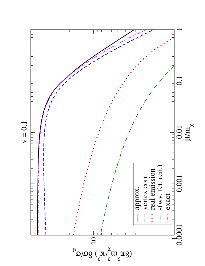
Figure 9: Normalized higher order contributions to the $\chi$ annihilation cross section for relative initial state velocity $v=0.1$. The solid (black) curve shows our approximation of Sec. 2, given by $I_{S}/v$. The dashed (blue), dotted (red) and dot–dashed (green) curves show exact contributions from vertex corrections, real emission diagrams, and wave function renormalization, respectively; the latter has to be multiplied with $-1$. The dash–doubledotted (magenta) curve shows the sum of these three contribution, i.e. the exact one–loop correction; it nearly coincides with the black curve for $\mu/m_{\chi}\leq 0.2$.

Fig. 9 shows that the sum of the vertex correction, wave function renormalization and real emission contributions very closely matches our approximate result of Sec. 2 for $\mu\raisebox{-3.69899pt}{~{}\shortstack{$<$ \\ [-0.07cm] $\sim$}}~{}0.5m_{\chi}$. In fact, the difference is always of order $\kappa^{2}/(8\pi^{2}m_{\chi}^{2})$, without any potentially large factors like $1/v$ or $\ln(m_{\chi}/\mu)$. We checked that this remains true at least for all $v\raisebox{-3.69899pt}{~{}\shortstack{$<$ \\ [-0.07cm] $\sim$}}~{}0.5$ relevant for the calculation of the relic density. It is not surprising that our approximate treatment does not treat such “generic” higher order contributions correctly. However, our approximation does closely resemble the exact result whenever the latter is large. This is all we aspired to, and in most cases all we need when calculating DM relic densities, even if PLANCK data reduce the uncertainty of the observed value to the percent level.

References

- [1] For a review, see G. Bertone, D. Hooper and J. Silk, Phys. Rept. 405 (2005) 279, hep-ph/0404175.
- [2] WMAP Collab., E. Komatsu et al., Astrophys. J. Suppl. 180 (2009) 330, arXiv:0803.0547 [astro-ph].
- [3] Planck Science Team, G. Efstathiou et al., “PLANCK: The Scientific Programme”, http://www.rssd.esa.int/SA/PLANCK/docs/Bluebook-ESA-SCI(2005)1_V2.pdf .
- [4] M. Cirelli, A. Strumia and M. Tamburini, Nucl. Phys. B787 (2007) 152, arXiv:0706.4071 [hep-ph]; J. March-Russell, S.M. West, D. Cumberbatch and D. Hooper, JHEP 0807 (2008) 058, arXiv:0801.3440 [hep-ph]; N. Arkani-Hamed, D.P. Finkbeiner, T.R. Slatyer and N. Weiner, Phys. Rev. D79 (2009) 015014, arXiv:0810.0713 [hep-ph]; J. March-Russell and S.M. West, Phys. Lett. B676 (2009) 133, arXiv:0812.0559 [astro-ph].
- [5] R. Iengo, JHEP 0905 (2009) 024, arXiv:0902.0688 [hep-ph].
- [6] S. Cassel, arXiv:0903.5307 [hep-ph].
- [7] J. Hisano, S. Matsumoto and M.M. Nojiri, Phys. Rev. Lett. 92 (2004) 031303, hep-ph/0307216; J. Hisano, S. Matsumoto, M.M. Nojiri and O. Saito, Phys. Rev. D71 (2005) 063528, hep-ph/0412403; J. Hisano, S. Matsumoto, M. Nagai, O. Saito and M. Senami, Phys. Lett. B646 (2007) 34, hep-ph/0610249.
- [8] M. Backovic and J.P. Ralston, Phys. Rev. D81 (2010) 056002, arXiv:0910.1113 [hep-ph].
- [9] K. Griest and D. Seckel, Phys. Rev. D43 (1991) 3191.
- [10] C. Itzykson and J.–B. Zuber, Quantum Field Theory, McGraw–Hill (1985).
- [11] M. Drees and M.M. Nojiri, Phys. Rev. D47 (1993) 376, hep-ph/9207234.
- [12] See e.g. L.D. Landau and E.M. Lifshitz, Quantum Mechanics, Pergamon Press (1977).
- [13] See e.g. E.W. Kolb and M.S. Turner, The Early Universe, Westview Press (1994).
- [14] N. Baro, F. Boudjema, and A. Semenov, Phys. Lett. B660 (2008) 550, arXiv:0710.1821 [hep-ph].
- [15] J.B. Dent, S. Dutta and R.J. Scherrer, Phys. Lett. B687 (2010) 275, arXiv:0909.4128 [astro-ph.CO]; J. Zavala, M. Vogelsberger and S.D.M. White, Phys. Rev. D81 (2010) 083502, arXiv:0910.5221 [astro-ph.CO].
- [16] J. Hisano, K. Kohri and M.M. Nojiri, Phys. Lett. B505 (2001) 169, hep-ph/0011216; S. Hofmann, D.J. Schwarz and H. Stoecker, Phys. Rev. D64 (2001) 083507, astro-ph/0104173.
- [17] C.P. Burgess, M. Pospelov and T. ter Veldhuis, Nucl. Phys. B619, (2001) 709, hep-ph/0011335.
- [18] H. Davoudiasl, R. Kitano, T. Li and H. Murayama, Phys. Lett. B609 (2005) 117, hep-ph/0405097.
- [19] E. Ma, Phys. Rev. D73 (2006) 077301, hep-ph/0601225; R. Barbieri, L.J. Hall and V.S. Rychkov, Phys. Rev. D74 (2006) 015007, hep-ph/0603188; L. Lopez Honorez, E. Nezri, J.F. Oliver and M.H.G. Tytgat, JCAP 0702 (2007) 028, hep-ph/0612275.
- [20] Y.G. Kim, K.Y. Lee and S. Shin, JHEP 0805 (2008) 100, arXiv:0803.2932 [hep-ph].
- [21] G. Jungman, M. Kamionkowski and K. Griest, Phys. Rept. 267 (1996) 195, hep-ph/9506380.
- [22] J.R. Ellis, T. Falk and K.A. Olive, Phys. Lett. B444 (1998) 367 (1998), hep-ph/9810360; J.R. Ellis, T. Falk, K.A. Olive and M. Srednicki, Astropart. Phys. 13 (2000) 181, Erratum-ibid. 15 (2001) 413, hep-ph/9905481; M.E. Gomez, G. Lazarides and C. Pallis, Phys. Rev. D61 (2000) 123512, hep-ph/9907261; C. Boehm, A. Djouadi and M. Drees, Phys. Rev. D62 (2000) 035012, hep-ph/9911496; J.R. Ellis, K.A. Olive and Y. Santoso, Astropart. Phys. 18 (2003) 395, hep-ph/0112113.
- [23] T.R. Slatyer, JCAP 1002 (2010) 028, arXiv:0910.5713 [hep-ph].
- [24] J. Edsjö and P. Gondolo, Phys. Rev. D56 (1997) 1879, hep-ph/9704361.
- [25] N. Arkani-Hamed, A. Delgado and G.F. Giudice, Nucl. Phys. B741 (2006) 108, hep-ph/0601041.
- [26] G. Bélanger, F. Boudjema, A. Pukhov and A. Semenov, Comput. Phys. Commun. 174 (2006) 577, hep-ph/0607059.
- [27] B.C. Allanach, Comput. Phys. Commun. 143 (2002) 305-331, hep-ph/0104145.
- [28] S. Mizuta and M. Yamaguchi, Phys. Lett. B298, 120 (1993).
- [29] N. Baro, F. Boudjema, G. Chalons and S. Hao, Phys. Rev. D81 (2010) 015005, arXiv:0910.3293 [hep-ph].
- [30] A. Freitas, Phys. Lett. B652 (2007) 280, arXiv:0705.4027 [hep-ph]; B. Herrmann and M. Klasen, Phys. Rev. D76 (2007) 117704, arXiv:0709.0043 [hep-ph]; B. Herrmann, M. Klasen and K. Kovarik, Phys. Rev. D79 (2009) 061701, arXiv:0901.0481 [hep-ph]; B. Herrmann, M. Klasen and K. Kovarik, Phys. Rev. D80 (2009) 085025, arXiv:0907.0030 [hep-ph].
- [31] K.A. Olive and D. Thomas, Nucl. Phys. B355 (1991) 192; S.A. Abel, S. Sarkar and I.B. Whittingham, Nucl. Phys. B392 (1993) 83, hep-ph/9209292; G. Bélanger, F. Boudjema, C. Hugonie, A. Pukhov, and A. Semenov, JCAP 0509 (2005) 001, hep-ph/0505142.
- [32] W. Beenakker, S.C. van der Marck and W. Hollik, Nucl. Phys. B365 (1991) 24.