Superfluid to Bose-glass transition of hard core bosons in one-dimensional incommensurate optical lattice

Abstract

We study superfluid to Anderson insulator transition of strongly repulsive Bose gas in a one dimensional incommensurate optical lattice. In the hard core limit, the Bose-Fermi mapping allows us to deal with the system exactly by using the exact numerical method. Based on the Aubry-André model, we exploit the phase transition of the hard core boson system from superfluid phase with all the single particle states being extended to the Bose glass phase with all the single particle states being Anderson localized as the strength of the incommensurate potential increasing relative to the amplitude of hopping. We evaluate the superfluid fraction, the one particle density matrices, momentum distributions, the natural orbitals and their occupations. All of these quantities show that there exists a phase transition from superfluid to insulator in the system.

I Introduction

Anderson localization Anderson was predicted fifty years ago as the localization of the electronic wave function in a disordered potential. So far the phenomenon of Anderson localization has been observed in variety of systems, such as electromagnetic waves Wiersma ; Dalichaouch , sound waves Weaver , and quantum matter waves Billy ; Roati ; Chabe ; Edwards . Recently lots of attentions have been payed on the cold atom systems in disordered potentials Modugno ; Adhikari because of the experimental realization of the Anderson localization of the quantum matter waves Billy ; Roati . The good tunability in ultracold atom systems Bloch offers myriad opportunities for studying the disorder effects in a controllable way. Random potential can be introduced by baser beams generating speckle patterns in the optical lattice Billy ; Lye . By this way, Billy et al. observed exponential localization of a Bose-Einstein condensate (BEC) of ⁸⁷Rb atoms released into a one-dimensional waveguide Billy . Also one can achieve the random potential by loading a mixture of two kinds of atoms in a optical lattice with one heavy and one light, and the effect of the heavy ones is to produce an effective random potential for the lighter atoms when the heavy ones localize in the lattice randomly Gavish . Another way to produce the random potential is to superimpose two one-dimensional (1D) optical lattices with incommensurate wave lengths to generate quasi-periodic potential Roati ; Fallani . Particularly, Roati et al. Roati observed localization of a noninteracting BEC of ³⁹K atoms in a 1D system with two optical lattice potentials.

On the other hand, the interactions between bosons in the cold atom systems can be controllably tuned by Feshbach resonances. It is thus feasible to experimentally study Roati1 the interplay between disorder and interactions in bosonic systems under controlled conditions, which has been a longstanding problem subjected to intensive studies. Theoretically, it has been predicted that there is a phase transition from a superfluid phase with extended single particle states to the Bose-glass (BG) phase Giamarchi ; Fisher1 ; Delande ; Fontanesi with Anderson localized single particle states. The study of the interplay of disorder and interaction in strongly interacting ultracold atomic systems also gets lots of attentions Orso ; Roux ; Deng ; Roscilde ; Gurarie . Despite the intensive studies Orso ; Roux ; Deng ; Roscilde ; Gurarie ; Scalettar ; Zhang ; Singh ; Rapsch , the properties of the disordered interacting bosons remain on debate. The theory of disordered interacting bosons is difficult and exact solutions are rarely known apart from numerical or approximate results. An exception is in the one-dimensional (1D) limit with infinitely strong repulsive interactions, where the disordered boson problem can be exactly solvable via a Bose-Fermi mapping Egger . In the present work, we study the interacting bosons in the incommensurate optical lattices in the limit with infinitely repulsive interaction. In this limit, the Bose gas is known as Tonks-Girardeau gas or hard core bosonic gas Girardeau , which has been experimentally realized Toshiya ; Paredes . The Bose-Fermi mapping or the Jordan-Winger transformation for hard-core bosons in 1D optical lattice establishes a connection to non-interacting disordered fermions, which greatly simplify the computation of physical quantities like the momentum distribution. Following an exact numerical approach proposed by Rigol and Muramatsu Rigol , we calculate the superfluid fractions, one particle density matrices, momentum distributions, natural orbitals and their occupations to exploit the phase transition of the system from superfluid to BG phase.

II Model

We consider $N$ hard-core ultra-cold bosons in a 1D incommensurate optical lattice. Under the single band tight binding approximation, the system can be described by the following hard core bosons Hamiltonian:

$$H=-t\sum_{i}(b^{\dagger}_{i}b_{i+1}+H.c.)+V\sum_{i}\mathrm{cos}(\alpha 2\pi i+\delta)n^{b}_{i}$$ (1)

where $b^{\dagger}_{i}(b_{i})$ is the creation (annihilation) operator of the boson and they satisfy the hard core constraints Rigol , i.e., the on-site anti-commutation $(\{b_{i},b^{\dagger}_{i}\}=1)$ and $[b_{i},b^{\dagger}_{j}]=0$ for $i\neq j$; $n^{b}_{i}$ is the bosonic particle number operator; $t$ is the amplitude of hopping and we will set it to be the unit of the energy $(t=1)$; $V$ is the strength of incommensurate potential with $\alpha$ being an irrational number characterizing the degree of the incommensurability and $\delta$ an arbitrary phase (in our calculation it is chosen to be zero for convenience, without loss of generality).

In order to obtain the ground state properties of the hard core bosons, we use the Jordan-Wigner transformation Jordan

$$b^{\dagger}_{j}=f^{\dagger}_{j}\prod^{j-1}_{\beta=1}e^{-i\pi f^{\dagger}_{\beta}f_{\beta}},b_{j}=\prod^{j-1}_{\beta=1}e^{+i\pi f^{\dagger}_{\beta}f_{\beta}}f_{j},$$ (2)

which maps the hard core bosons Hamiltonian into a noninteracting spinless fermions Hamiltonian

$$H=-\sum_{i}(f^{\dagger}_{i}f_{i+1}+H.c.)+V\sum_{i}\mathrm{cos}(\alpha 2\pi i)n^{f}_{i}$$ (3)

where $f^{\dagger}_{i}(f_{i})$ is the creation (annihilation) operator of the spinless fermion and $n^{f}_{i}$ is the particle number operator. The ground state wave function of the $N$ spinless free fermionic system can be obtained by diagonalizing Eq.(3) and be written as:

$$|\Psi^{G}_{F}\rangle=\prod^{N}_{n=1}\sum^{L}_{i=1}P_{in}f^{\dagger}_{i}|0\rangle$$ (4)

where $L$ is the number of the lattice sites, $N$ is the number of fermions (same as bosons), and the matrix $P$ is given by the lowest $N$ eigenfunctions of the Hamiltonian,

$$P=\left(\begin{array}[]{cccc}P_{11}&P_{12}&\cdots&P_{1N}\\ P_{21}&P_{22}&\cdots&P_{2N}\\ \vdots&\vdots&&\vdots\\ P_{L1}&P_{L2}&\cdots&P_{LN}\end{array}\right)$$ (5)

with all the rows being ordered starting from the one with the lowest energy.

The solution of $P_{in}$ reduces to a single particle problem. The motion of a single particle in a 1D lattice can be described by the nearest neighbor tight binding equation

$$u_{i+1,n}+u_{i-1,n}+V_{i}u_{i,n}=E_{n}u_{i,n},$$ (6)

where the amplitude of the nearest neighbor hopping has been set to be unity, $u_{i,n}=P_{in}$ is the amplitude of the particle wave function at $i$ site with $V_{i}$ the on site diagonal potential and $E_{n}$ is the $n$-th single particle eigen energy with the eigen state given by $|n\rangle=\sum_{i}u_{i,n}f_{i}^{\dagger}|0\rangle$. Obviously the solution to Eq. (6) is dependent on the potential $V_{i}$. For periodic $V_{i}$ Bloch’s theorem tells us that all the single particle states are extended band states. For a random $V_{i}$ the system is the Anderson model and Eq.(6) produces Thouless localized states in 1D. For the incommensurate case $V_{i}=V\mathrm{cos}(2\pi\alpha i)$ with irrational $\alpha$, Eq.(6) is the well-known Aubry-André model Aubry . Aubry and André showed that when $V<2$ all the single particle states are extended and when $V>2$ all the single particle states are the localized states. Mobility edges also have been found for the extended Aubry-André model Sarma ; Biddle .

III Transition from superfluid to Bose-glass phase

To see whether a bosonic system is in a superfluid phase, we can calculate the superfluid fraction, which reflects the response of a superfluid to the imposed phase gradient. Generally a nonzero superfluid fraction $f^{N}_{s}$ characterizes the system being in the superfluid phase. The superfluid fraction can be calculated with the aid of Peierls phase factors introduced in the Hamiltonian Eq.(1) by means of the replacement $b^{\dagger}_{i}b_{i+1}\rightarrow b^{\dagger}_{i}b_{i+1}e^{i\varphi}$. In terms of free energy $F_{N}(\varphi)$ for very small $\varphi$, the superfluid fraction is then determined as Roth ; Fisher

$$f^{N}_{s}=\underset{\varphi\rightarrow 0}{\mathrm{lim}}\tfrac{F_{N}(\varphi)-F_{N}(0)}{t\varphi^{2}N}.$$ (7)

For hard core bosons in one dimension, the above expression can be represented as Krutitsky

$$f^{N}_{s} = \tfrac{1}{2N}\sum^{L}_{i=1}\sum^{N}_{n=1}[u^{*}_{i,n}u_{i+1,n}+c.c]$$ (8)

$$-\tfrac{1}{N}\sum^{L}_{n=N+1}\sum^{N}_{m=1}\tfrac{1}{E_{n}-E_{m}}|\sum^{L}_{i=1}[u^{*}_{i,n}u_{i+1,m}$$

$$-u^{*}_{i+1,}u_{i,m}]|^{2},$$

with $u_{L+1,n}=(-1)^{N+1}u_{1,n}$ and $E_{n}$ is the eigenenergy of the $n$-th row in $P$ matrix. The results of numerical calculations for the superfluid fractions for the hard core bosons in incommensurate lattices are shown in Fig.1 for three different lattice sizes and fillings. Here we consider odd numbers of bosons and use periodic boundary conditions Lieb . When the strength of the incommensurate potential $V$ is small, the system is in the superfluid phase with nonzero superfluid fraction. As $V$ increases, the incommensurate potential acting as a pseudo-random potential makes the bosons difficult to hop and tend to be localized. Consequently, the superfluid fraction decreases. When $V$ gets around $2$, the superfluid fraction approaches zero, and the system is in the Bose glass phase (insulating phase) with all the bosons being localized Fontanesi . We note that with different irrational $\alpha$ and fillings the curves of superfluid fraction exhibit similar behavior.

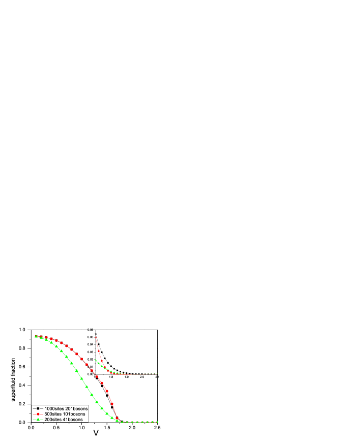
Figure 1: (Color online)The superfluid fraction versus $V$ (the strength of the incommensurate potential) for three different lattice sizes and fillings with $\alpha=(\sqrt{5}-1)/2$. Insert: enlargement of picture around the critical point.

Figure 2: (Color online) Log-Log plots of the mean one particle density matrices for different $V$ of the systems with 201 bosons on 1000 lattice sites and $\alpha=(\sqrt{5}-1)/2$. The red straight line shows a power-law fit ($\overline{\rho}_{i}=0.195/\sqrt{i}$) for the mean one particle density matrix with $V=1.1$. Insert: The log-line plot of the mean one particle density matrix for $V=2.1$, and the red straight line shows an exponential-law fit ($\mathrm{ln}\overline{\rho}_{i}=-5.697-0.055i$) for the mean one particle density matrix.

The one particle Green’s function for the hard core bosons can be written in the form

$$G_{ij} = \langle\Psi^{G}_{HCB}|b_{i}b^{\dagger}_{j}|\Psi^{G}_{HCB}\rangle$$

$$= \langle\Psi^{A}|\Psi^{B}\rangle$$

where $|\Psi^{G}_{HCB}\rangle$ is the ground state of hard core bosons, and $\langle\Psi^{A}|=\left(f^{\dagger}_{i}\prod_{\beta=1}^{i-1}e^{-i\pi f^{\dagger}_{\beta}f_{\beta}}|\Psi^{G}_{F}\rangle\right)^{\dagger}$, $|\Psi^{B}\rangle=f^{\dagger}_{j}\prod_{\gamma=1}^{j-1}e^{-i\pi f^{\dagger}_{\gamma}f_{\gamma}}|\Psi^{G}_{F}\rangle$. After a straightforward evaluation, the state $\left|\Psi^{A}\right\rangle$ can be written as

$$\left|\Psi^{A}\right\rangle=\prod_{n=1}^{N+1}\sum_{l=1}^{L}P_{ln}^{A}f_{l}^{\dagger}\left|0\right\rangle$$

with $P_{ln}^{A}=-P_{ln}$ for $l\leq i-1$, $P_{ln}^{A}=P_{ln}$ for $l\geq i$ with $n\leq N$, $P_{iN+1}^{A}=1$ and $P_{lN+1}^{A}=0$ $\left(l\neq i\right)$, i.e., $P^{A}$ is formed by changing the sign of the elements $P_{ln}$ for $l<i$ because of the exponential term of the Jordan-Wigner transformation, and adding a column to $P$ with element $P_{iN+1}=1$ and all the others equal to zero for the further creation of a particle at site $i$. In the same way we can get $P^{B}$ for the state $|\Psi^{B}\rangle$ which has the same form as $\left|\Psi^{A}\right\rangle$ with the replacement of $i$ by $j$. The Green’s function is a determinant dependent on the $L\times\left(N+1\right)$ matrices $P^{A}$ and $P^{B}$ Rigol

$$G_{ij}=\left\langle\Psi^{A}|\Psi^{B}\right\rangle=\det\left[\left(P^{A}\right)^{\dagger}P^{B}\right].$$ (10)

It follows that the one particle density matrix can be determined by the expression

$$\rho_{ij}=\langle b^{\dagger}_{i}b_{j}\rangle=G_{ij}+\delta_{ij}(1-2G_{ii}).$$ (11)

Then we define the mean one particle density matrix as

$$\overline{\rho}_{i}=\tfrac{1}{L}\sum^{L}_{j=1}\rho_{j,j+i-1}$$ (12)

to reduce the drastic oscillations caused by the incommensurate potential. The mean one particle density matrices for different $V$ are shown in Fig.2. The mean one particle density matrices for $V<1.1$ are almost the same as the one with $V=1.1$, having the power-law decay with exponent of $-1/2$, which has the same exponent of the hard core bosons in the lattice without the incommensurate potential Rigol . As $V$ increases further, the mean one particle density matrix still has power-law decay, but the exponent is smaller than $-1/2$. Correspondingly the superfluid fraction decreases fast (see Fig.1). When $V$ exceeds the critical point, the mean one particle density matrix has the exponential-law decay which is the character of the Bose glass phase.

Figure 3: Momentum distributions for systems with 1000 lattice sites, $\alpha=(\sqrt{5}-1)/2$, V=1.1, and fillings of 201 (a), 501 (b), 801 (c) hard core bosons. (d): The value of the tail of momentum distributions relates to the number of bosons ($N$) for systems with 1000 lattice sites, $\alpha=(\sqrt{5}-1)/2$ and V=1.1.

The momentum distribution is defined by the Fourier transform with respect to $i-j$ of the one particle density matrix with the form

$$n(k)=\tfrac{1}{L}\sum^{L}_{i,j=1}e^{-ik(i-j)}\rho_{ij},$$ (13)

where $k$ denotes the momentum. In Fig. 3 we show the momentum distributions for systems with three different fillings in 1000 lattice sites. Odd numbers of particles are taken for periodic boundary conditions. The peak structure in the momentum distributions reflects the bosonic nature of the particles, which is in contrast with the structure of the momentum distributions of the equivalent noninteracting fermions. Also because of the existence of the additional lattice to produce the incommensurate potential, it is possible that there exist other peaks besides at $k=0$ in the momentum distributions. For $\alpha=(\sqrt{5}-1)/2$, the secondary peaks are found to appear at $k=\pm(\alpha-1)2\pi$ only for low and high fillings. On increasing the number of the bosons the population of the high momenta states is always increasing, which leads to the increase in the tails of the momentum distribution as shown in Fig.3d.

Figure 4: Momentum distributions for systems with 1000 lattice sites, $\alpha=(\sqrt{5}-1)/2$, 201 hard core bosons, and $V=1.1$ (a); $V=1.7$ (b); $V=2.3$ (c). (d): The value of secondary peaks of momentum distributions relates to $V$ for systems with 1000 lattice sites, 201 bosons and $\alpha=(\sqrt{5}-1)/2$. (e): The position of the secondary peak (the $k>0$ one) in the momentum distributions relates to $\alpha^{\prime}$ for systems with 1000 lattice sites, 201 hard core bosons, and $V=1.1$. The irrational numbers beside the points are the corresponding $\alpha$.

Then we consider the properties of the momentum distributions as the strength of the incommensurate potential changing. In Fig.4 we show the momentum distributions for systems with three different $V$. Low fillings are required for the existence of secondary peaks in the momentum distributions. On increasing $V$, the value of $n_{k=0}$ decreases which means that the coherence among the hard core bosons decreases and the superfluid fraction decreases. Also the peak at $k=0$ and the secondary peaks all become widespread. The value of the secondary peaks (Fig.4d) first increases, and it starts to decrease when $V$ is bigger than around $1.5$. Finally it reaches an almost fixed number as the system going into the BG phase. The population of high momenta states is always increasing accompanying the decrease of the peak at $k=0$.

Figure 5: Occupations of the natural orbitals for systems with 1000 lattice sites, 201 bosons, $\alpha=(\sqrt{5}-1)/2$ and $V=0$ (a); $V=1.5$ (b); $V=2.3$ (c). (d): The amplitude of the discontinuation ($Z$) defined as $Z=\lambda_{N}-\lambda_{N+1}$ relates to $V$ for systems with 1000 lattice sites, 201 bosons and $\alpha=(\sqrt{5}-1)/2$.

Now we consider the properties of the secondary peaks. Their positions are only decided by the value of $\alpha$ and are irrelevant with the system size, $V$ and filling. But the existence of the secondary peaks are related to the filling, and the peaks only exist for low and high fillings. For the incommensurate lattice with the form $\mathrm{cos}(2\pi\alpha i)$, actually we can restrict $\alpha$ in the range of $[0,0.5]$ because $\mathrm{cos}[2\pi(\alpha-1)i]=\mathrm{cos}(2\pi\alpha i)$ and $\mathrm{cos}(-2\pi\alpha i)=\mathrm{cos}(2\pi\alpha i)$. For example, $\alpha=(\sqrt{5}\pm 1)/2$ are the same for the system. So any $\alpha\in(-\infty,\infty)$ has an equivalent number in the range $[0,0.5]$, and we denote it by $\alpha^{\prime}$. The positions of the secondary peaks are decided by the value of $\alpha^{\prime}$. In Fig.4e we show the position of the secondary peak (the $k>0$ one) as a function of $\alpha^{\prime}$. From the data we can see that the positions of the secondary peaks in the momentum distribution are decided by $\alpha$ and at $k=\pm 2\alpha^{\prime}\pi$.

Figure 6: Profiles of the two lowest natural orbitals for systems with 1000 lattice sites, 201 bosons, $\alpha=(\sqrt{5}-1)/2$ and $V=0$ (a)(b); $V=1.5$ (c)(d); $V=2.3$ (e)(f).

Figure 7: The condensate fraction $f_{c}$ versus $V$ for systems with 1000 lattice sites, 201 bosons, and $\alpha=(\sqrt{5}-1)/2$.

The natural orbitals $(\phi^{\eta}_{i})$ are defined as the eigenfunctions of the one particle density matrix Penrose ,

$$\sum^{L}_{j=1}\rho_{ij}\phi^{\eta}_{j}=\lambda_{\eta}\phi^{\eta}_{i},$$ (14)

and can be understood as being effective one particle states with occupations $\lambda_{\eta}$. For noninteracting bosons, all the particles occupy in the lowest natural orbital and bosons are in the BEC phase at zero temperature (only the quasi condensation exists for the 1D hard core bosons). The occupations of the natural orbitals for systems with three different $V$ are shown in Fig.5. The occupations are plotted versus the orbital numbers $\eta$, and ordered starting from the highest occupied one. For $V<2$, the occupation distribution exhibits sharp single-peak structure. The peak appearing in the lowest orbital is the feature of the boson which is against the step function of the fermions. With the increase in the strength of incommensurate potential, the occupation of the lowest natural orbital ($\lambda_{1}$) decreases. When $V>2$, no an obvious peak appears in the lowest natural orbital. We also find that a discontinuation at $\eta=N$ emerges when $V>2$. To characterize such a discontinuation, we define $Z=\lambda_{N}-\lambda_{N+1}$ which indicates the occupation difference between the $N$-th and $(N+1)$-th natural orbital for a boson system with $N$ particles. The amplitude of the discontinuation Z versus the strength of the incommensurate potential ($V$) is plotted in Fig.5d. There is an obvious change around $V=2$. For $V<2$ there is no discontinuation in the occupation number. However, for $V>2$ a nonzero Z appears and the amplitude of the discontinuation increases with the increase in $V$.

The effect of incommensurate potential on the natural orbital is shown in Fig.6, where profiles of the two lowest natural orbitals for the same system with three different $V$ are plotted. When $V=0$, there is only the periodic optical lattice, and the natural orbitals are plane waves. As $V$ increases but is smaller than $2$, the natural orbitals still spread over all the lattice corresponding to extended states, but there are a lot oscillations in the waves induced by the existence of the incommensurate potential which acts like random potential on sites because of the irrational $\alpha$. When $V>2$ the states do not spread over all the lattice any more and are localized. Correspondingly the system is in the BG phase.

Finally we consider the influence of incommensurate potential on the condensate fraction, which is defined as $f_{c}=\lambda_{1}/N$ to indicate the ratio of occupation of lowest natural orbital. In Fig.7 we show the condensate fraction as function of $V$. For small $V$ the condensate fraction $f_{c}$ decreases slowly with the increase in $V$. As $V$ increases further to approach $V=2$, the condensate fraction decreases rapidly. For $V>2$ there is almost no condensation. The change of the condensate fraction also gives signature of the superfluid to insulator transition in the incommensurate optical lattice system.

IV Summary

In summary, we have studied the properties of hard core bosons in an incommensurate optical lattice. Using the Bose-Fermi mapping and the exact numerical method proposed by Rigol and Muramatsu Rigol , we exploit the phase transition from superfluid to the localized BG phase as the strength of the incommensurate potential increases from weak to strong. We calculate the superfluid fraction, one particle density matrices, momentum distributions, the natural orbitals and their occupations. All of these quantities show that there exists a phase transition in the system when the strength of incommensurate potential exceeds $V=2$. Our study provides an exact example which unambiguously exhibits the transition from superfluid to Anderson insulator in an incommensurate optical lattice.

- (1) P. W. Anderson, Phys. Rev. 109, 1492 (1958).
- (2) D. S. Wiersma et al., Nature (London) 390, 671 (1997); F. Scheffold et al., ibid 398,206 (1999).
- (3) R. Dalichaouch et al., Nature (London) 354, 53 (1991); A.A.Chabanov et al., ibid 404, 850 (2000).
- (4) R. L. Weaver et al., Wave Motion 12, 129 (1990).
- (5) J. Billy et al., Nature (London) 453, 891 (2008).
- (6) G. Roati et al., Nature (London) 453, 895 (2008).
- (7) J. Chabé, G.Lemarie, B.Gremaud, D.Delande, P.Szriftgiser, and J.C.Garreau, Phys. Rev. Lett. 101, 255702 (2008).
- (8) E. E. Edwards, M. Beeler, T. Hong, and S. L. Rolstion, Phys. Rev. Lett. 101, 260402 (2008).
- (9) M. Modugno, New J. Phys. 11, 033023 (2009).
- (10) S. K. Adhikari, and L. Salasnich, Phys. Rev. A. 80, 023606 (2009).
- (11) I. Bloch, J. Dalibard, and W. Zwerger, Rev. Mod. Phys. 80, 885 (2008).
- (12) J. E. Lye et al., Phys. Rev. Lett. 95, 070401 (2005); D. Clément et al., Phys. Rev. Lett. 95, 170409 (2005); C. Fort et al., Phys. Rev. Lett. 95, 170410 (2005); T. Schulte et al., Phys. Rev. Lett. 95, 170411 (2005); Y. P. Chen et al., Phys. Rev. A. 77, 033632 (2008)
- (13) U. Gavish and Y. Castin, Phys. Rev. Lett. 95, 020401 (2005).
- (14) L. Fallani, J. E. Lye, V. Guarrera, C. Fort, and M. Inguscio, Phys. Rev. Lett. 98, 130404 (2007).
- (15) G. Roati et al., Phys. Rev. Lett. 99, 010403 (2007).
- (16) T. Giamarchi and H. J. Schulz, Phys. Rev. B. 37, 325 (1988); Europhys. Lett. 3, 1287 (1987).
- (17) M. P. Fisher et al., Phys. Rev. B. 40, 546 (1989).
- (18) D. Delande and J. Zakrzewshi, Phys. Rev. Lett. 102, 085301 (2009).
- (19) L. Fontanesi, M. Wouters, V. Savona, Phys. Rev. Lett. 103, 030403 (2009).
- (20) V. Gurarie, L. Pollet, N. V. Prokofev, B. V. Svistunov, and M. Troyer, arXiv: 0909.4593; L. Pollet, N. V. Prokofev, B. V. Svistunov, and M. Troyer, arXiv: 0903.3867. B. V. Svistunov, Phys. Rev. B 54, 16131 (1996).
- (21) G. Roux et al., Phys. Rev. A. 78, 023628 (2008).
- (22) X. Deng et al., Phys. Rev. A. 78, 013625 (2008).
- (23) T. Roscilde, Phys. Rev. A. 77, 063605 (2008).
- (24) G. Orso, Phys. Rev. Lett. 99, 250402 (2007); G. Orso, A. Iucci, M. A. Cazalilla, T. Giamarchi, Phys. Rev. A 80, 033625 (2009).
- (25) R. T. Scalettar, G. G. Batrouni, and G. T. Zimanyi, Phys. Rev. Lett. 66, 3144 (1991).
- (26) L. Zhang and M. Ma, Phys. Rev. B 45, 4855 (1992).
- (27) K. G. Singh and D. S. Rokhsar, Phys. Rev. B 46, 3002 (1992).
- (28) S. Rapsch, U. Schollwöck, and W. Zwerger, Europhys. Lett. 46, 559 (1999).
- (29) A. De Martino, M. Thorwart, R. Egger, and R. Graham, Phys. Rev. Lett. 94, 060402 (2005).
- (30) M. Girardeau, J. Math. Phys 1, 1268 (1960).
- (31) B. Paredes et al., Nature (London) 429, 277 (2004).
- (32) T. Kinoshita, et. al., Science 305, 1125 (2004).
- (33) M. Rigol and A. Muramatsu, Phys. Rev. A. 72, 013604 (2005); M. Rigol and A. Muramatsu, Phys. Rev. A. 70, 031603(R) (2004).
- (34) P. Jordan and E. Wigner, Z.Phys. 47, 631 (1928).
- (35) D. J. Thouless, Phys. Rep. 13, 95 (1974); P. A. Lee and T. V. Ramakrishnan, Rev. Mod. Phys. 57, 287 (1985).
- (36) A. Aubry and G. André, Ann. Israel Phys. Soc 3, 133 (1980).
- (37) S. Das Sarma, S. He, and X. C. Xie, Phys. Rev. Lett. 61, 2144 (1988); S. Das Sarma, S. He, and X. C. Xie, Phys. Rev. B. 41, 5544 (1990).
- (38) J. Biddle et al., Phys. Rev. A 80, 021603 (2009).
- (39) R. Roth and K. Burnett, Phys. Rev. A. 67, 031602(R) (2003); R. Roth and K. Burnett, ibid. 68, 023604 (2003).
- (40) M. E. Fisher, M. N. Barber, and D. Jasnow, Phys. Rev. A. 8, 1111 (1973); W.Krauth, Phys. Rev. B. 44, 9772 (1991).
- (41) K. V. Krutitsky, M. Thorwart, R. Egger and R. Graham, Phys. Rev. A. 77, 053609 (2008).
- (42) E. Lieb, T. Shultz and D. Mattis, Ann. Phys. (N.Y.) 16, 406 (1961).
- (43) O. Pensose and L. Onsager, Phys. Rev. 104, 576 (1956).