Nonequilibrium fluctuation theorems in the presence of a time-reversal symmetry-breaking field and nonconservative forces

Abstract

We study nonequilibrium fluctuation theorems for classical systems in the presence of a time-reversal symmetry-breaking field and nonconservative forces in a stochastic as well as a deterministic set up. We consider a system and a heat bath, called the combined system, and show that the fluctuation theorems are valid even when the heat bath goes out of equilibrium during driving. The only requirement for the validity is that, when the driving is switched off, the combined system relaxes to a state having a uniform probability measure on a constant energy surface, consistent with microcanonical ensemble of an isolated system.

I Introduction

Understanding thermodynamics of irreversible processes from time reversible microscopic dynamics has been a subject of great interest since the time of foundation of statistical physics. A fair amount of progress has been made since then, especially through the recently discovered fluctuation theorems Evans ; review1 ; review2 ; review3 ; Evans_Searles ; Gallavotti . The fluctuation theorems give a quantitative measure of irreversibility in terms of asymmetries in the probability distributions of various quantities in a driven system, e.g., heat produced in a sheared fluid Evans ; Evans_Searles ; Gallavotti , heat exchanged between a hot and a cold body being in contact JarzynskiPRL2004 ; SaitoPRL2007 , etc. These nonequilibrium quantities, usually termed as ‘entropy production’ in an irreversible process Kurchan ; Lebowitz ; Sasa ; Maes ; Seifert , are on average non-negative and give an insight into the 2nd law of thermodynamics. The fluctuation theorem was originally derived for deterministic thermostatted dynamics Gallavotti and later for stochastic one, such as Langevin dynamics Kurchan and Markovian jump processes Lebowitz .

Closely connected to the fluctuation theorems, there are two remarkable relations, called the Jarzynski equality JarzynskiPRL1997 ; Park_Schulten ; Dellago and the Crooks theorem CrooksPRE1999 , which involve fluctuation of work done on a system driven arbitrarily far away from equilibrium by varying an external parameter. Consider a system which is initially at an equilibrium state ${\cal A}$ at temperature $T$ and coupled to an external parameter $\lambda(t)$. The system is driven out of equilibrium by varying $\lambda(t)$ in a time interval $0\leq t\leq\tau$ where $\lambda(t)$ is constant outside this time interval. In this process, called forward process for a fixed protocol $\lambda(t)$, an amount of work $W$ is done on the system. The system eventually relaxes to an equilibrium state ${\cal B}$ at same temperature $T$. In the reverse process, the system is driven from the initial equilibrium state ${\cal B}$ for a reverse protocol $\lambda(\tau-t)$ and eventually the system relaxes to the equilibrium state ${\cal A}$. The Jarzynski equality relates average of $\exp(-\beta W)$ performed over nonequlibrium trajectories to equilibrium free energy difference $\Delta F=F({\cal B})-F({\cal A})$ as

$$\langle\exp(-\beta W)\rangle=\exp(-\beta\Delta F)$$ (1)

where $F({\cal A})$ and $F({\cal B})$ are equilibrium free energy of the system at state ${\cal A}$ and ${\cal B}$ respectively, and $\beta=1/k_{B}T$, $k_{B}$ the Boltzmann constant. The Crooks theorem relates the ratio of the probabilities of work done $W$ for the forward process and that for the reverse process,

$$\frac{P_{F}(W)}{P_{R}(-W)}=e^{\beta(W-\Delta F)}$$ (2)

where $P_{F}(W)$ and $P_{R}(W)$ are the probability distributions of work for the forward and the reverse processes, respectively.

Dissipative mechanism of a heat bath is crucial for understanding irreversible phenomena and the fluctuation theorems Blythe , and is modeled in various ways, such as, by employing deterministic thermostatted dynamics Evans_Searles ; Gallavotti , stochastic Langevin dynamics satisfying the fluctuation-dissipation theorem Kurchan ; Narayan ; Mai_Dhar ; Speck_Seifert or Markov dynamics satisfying detailed balance with respect to canonical measure CrooksPRE1999 ; Crooks2000 . However in these cases, the heat bath is not considered explicitly, and is assumed to be always in equilibrium. In a realistic scenario, heat generated by a driving force is continuously dissipated to the heat bath, and consequently the portion of the heat bath in the vicinity of the system goes away from equilibrium during driving CohenJStatMech ; CohenMolPhys .

It is therefore important how one employs a heat bath to take into account the nonequilibrium effect of the bath. Recently there is a prescription of modeling a driven system, possibly in contact with a nonequilibrium heat bath, by applying Jaynes’ principle of entropy-maximization Jaynes to nonequilibrium trajectories with a macroscopic flux constraint RMLEvans_PRL ; RMLEvans_JPhysA ; Simha . However we follow a different path where we explicitly consider a system and a heat bath combined, either obeying microscopic Newtonian dynamics or obeying stochastic dynamics with symmetries of the microscopic Newtonian dynamics preserved. The work fluctuation relations have been studied along this line before for classical Hamiltonian dynamics Jarzynski_JStatPhys ; Broeck as well as stochastic dynamics Pradhan , but any time-reversal symmetry-breaking fields or nonconservative forces have not been considered. Recently, the fluctuation theorem involving particle-current has been studied in a case of quantum mechanical transport of electrons across a quantum dot in the presence of a time-independent magnetic field Saito_Utsumi .

In this paper, we generalize the fluctuation theorems for classical systems in the presence of a time-reversal symmetry-breaking field, such as an external magnetic field, and nonconservative forces which cannot be derived from gradient of scalar potentials. We consider a system and a heat bath, combined, in a deterministic as well as a stochastic set up and we show that the fluctuation theorems are valid in the presence of time-reversal symmetry-breaking fields and nonconservative forces, even when the heat bath goes out of equilibrium during the driving. The validity only requires that (1) in the absence of driving the system and the heat bath, combined, relax to a state with a uniform probability measure on a constant energy surface, and (2) there exists a time-reversal operation under which work performed on the system is odd. Although we specifically consider an external magnetic field in the paper, the results are also applicable to other time-reversal symmetry-breaking fields, e.g., a Coriolis force present in a rotating system.

In a deterministic set up, we consider a system obeying Newtonian dynamics and we prove the fluctuation theorems using the fact that Liouville’s theorem is valid even in the presence of an external time-dependent magnetic field as well as other nonconservative forces. We also extend our analysis to stochastic dynamics in the presence of a time-reversal symmetry-breaking field in a microcanonical set up. We consider an isolated system governed by Markovian dynamics where there is violation of detailed balance with respect to a uniform measure, i.e., forward and corresponding reverse transition probabilities are not equal in general. Reversing the time-reversal symmetry-breaking field results in dynamics where all forward and corresponding reverse transition probabilities are interchanged with each other. Although detailed balance is violated, we prove the fluctuation theorems only requiring that the steady state measure of an isolated system is uniform on a constant energy surface.

We primarily focus on the work fluctuation relations, i.e., the Jarzynski equality and the Crooks fluctuation theorem. The system is driven by varying a control parameter of an external potential or (and) by nonconservative forces. For systems obeying Newtonian dynamics, the driving force may be due to a nonconservative electric field induced by an external time varying magnetic field in addition to other nonconservative forces. The work fluctuation theorems have recently been studied for a few specific cases of a single Brownian particle in the presence of both time-independent Jayannavar ; Roy and time-dependent Saha_Jayannavar magnetic field. However we formulate the problem in a more general setting, taking into account the system and the heat bath degrees of freedom explicitly. Note that our analysis is applicable only to the classical systems consisting of particles which do not have any intrinsic magnetic moment.

Here is a brief outline of the paper. In section II, we study systems obeying Newtonian dynamics in the presence of an external magnetic field and some other nonconservative force fields. In section III, we give a general proof of the fluctuation theorems for stochastic systems in the absence of detailed balance in a microcanonical set up, in section IV we then illustrate the ideas using two simple stochastic models. In section V, we generalize the results for other intensive thermodynamic variables, e.g., pressure and chemical potential which determine the initial and final equilibrium states of the system in contact with a heat bath.

II Newtonian dynamics

First, we study the nonequilibrium fluctuation theorems in a general deterministic framework for a system and a heat bath combined, called the combined system (CS). We consider the CS, which is governed by microscopic Newtonian dynamics, in the presence of an external magnetic field $\vec{B}(\vec{r},t)$ and a nonconservative force field $\vec{f}(\vec{r},t)$. Force fields in general may be dependent both on position $\vec{r}$ and time $t$. The nonconservative force $\vec{f}(\vec{r},t)$ cannot be derived from gradient of a scalar potential. In addition, there may be conservative forces present in the CS which can be derivable from gradient of scalar potentials. A microstate of the CS is denoted by a variable ${\bf Y}$ which contains positions and velocities of all particles, i.e., ${\bf Y}\equiv(\vec{r}_{1},\vec{r}_{2},\dots,\vec{v}_{1},\vec{v}_{2},\dots)\equiv\{\vec{r}_{i},\vec{v}_{i}\}$ where $\vec{r}_{i}$ and $\vec{v}_{i}$ are position and velocity of $i$-th particle in the CS respectively. Newton’s equations of motion for $i$-th particle can be written as

$$\dot{\vec{r}}_{i}=\vec{v}_{i}\mbox{~{},~{}~{}~{}~{}~{}~{}~{}~{}~{}~{}~{}~{}~{}~{}~{}~{}~{}~{}~{}~{}~{}~{}~{}~{}~{}~{}~{}~{}~{}~{}~{}~{}~{}~{}~{}~{}~{}~{}~{}~{}}$$ (3)

$$m_{i}\dot{\vec{v}}_{i}=-\vec{\nabla}_{\vec{r}_{i}}V(\vec{r}_{i},\lambda(t))+q_{i}\vec{v}_{i}\times\vec{B}(\vec{r}_{i},t)$$

$$-q_{i}\frac{\partial\vec{A}(\vec{r}_{i},t)}{\partial t}+\vec{f}(\vec{r}_{i},t)$$ (4)

where $m_{i}$ and $q_{i}$ are mass and charge of the $i$-th particle, $V(\vec{r},\lambda(t))$ is total scalar potential at position $\vec{r}$ due to the inter-particle interaction potentials as well as an external potential with a time-dependent control parameter $\lambda(t)$, $\vec{\nabla}_{\vec{r}_{i}}$ the gradient operator with respect to coordinate $\vec{r}_{i}$, $\vec{A}(\vec{r},t)$ is the vector potential at position $\vec{r}$ and time $t$ due to the external magnetic field $\vec{B}(\vec{r},t)$ which can be written as curl of the vector potential, i.e., $\vec{B}(\vec{r},t)=\nabla\times\vec{A}(\vec{r},t)$. The third term in the r.h.s. of Eq. 4 is due to the time varying magnetic field $B(\vec{r},t)$ which induces a nonconservative electric field, $-{\partial\vec{A}}/{\partial t}$. The induced electric field, like $f(\vec{r},t)$, cannot be derived from gradient of a scalar potential.

It is important to note that, when the nonconservative force field $f(\vec{r},t)$ is present, there is no Hamiltonian for the CS and consequently Eqs. 3, 4 cannot be derived using a familiar Hamiltonian prescription of classical mechanics Goldstein . However the microscopic Newtonian equations of motion are still invariant under time-reversal with the direction of the magnetic field also reversed, i.e., as $t\rightarrow-t$, $\vec{v}_{i}\rightarrow-\vec{v}_{i}$ and $\vec{B}(\vec{r})\rightarrow-\vec{B}(\vec{r})$ (equivalently $\vec{A}(\vec{r})\rightarrow-\vec{A}(\vec{r})$), Eqs. 3 and 4 remain unchanged. Therefore, for any trajectory ${\bf Y}(t)\equiv\{\vec{r}_{i}(t),\vec{v}_{i}(t)\}$ with a fixed protocol $\{\lambda(t),\vec{B}(\vec{r},t),\vec{f}(\vec{r},t)\}$ in a time range $-{\cal T}\leq t\leq{\cal T}$, there exists a reverse trajectory $\tilde{{\bf Y}}(t)\equiv\{\vec{r}_{i}(-t),-\vec{v}_{i}(-t)\}$ for the corresponding reverse protocol $\{\lambda(-t),-\vec{B}(\vec{r},-t),\vec{f}(\vec{r},-t)\}$. Note that in the time-reversal operation mentioned above, direction of the nonconservative forces, $f$ as well as $-{\partial A}/{\partial t}$, are unchanged.

In the subsequent discussions, we consider a process in a time interval $-{\cal T}\leq t\leq{\cal T}$ where ${\cal T}$ is very large compared to any other time scales. We assume that the magnetic field $\vec{B}(\vec{r},t)$, the external parameter $\lambda(t)$ and the nonconservative force field $\vec{f}(\vec{r},t)$ couple only to the system. The field $\vec{B}(\vec{r},t)$ (or equivalently the vector potential $\vec{A}(\vec{r},t)$), $\lambda(t)$ and $\vec{f}(\vec{r},t)$ are varied according to a fixed protocol only in time interval $0\leq t\leq\tau$ where $\tau\ll{\cal T}$. Otherwise $\vec{B}$, $\lambda$ are kept constant and $\vec{f}=0$ outside the interval $0\leq t\leq\tau$.

Although there is no Hamiltonian in the presence of nonconservative forces, energy function of the CS, in terms of positions and velocities, can be defined as

$$E(\{\vec{r}_{i},\vec{v}_{i}\})=\left(\sum_{i}\frac{1}{2}m_{i}\vec{v}_{i}^{2}\right)+V(\{\vec{r}_{i}\},\lambda(t)),$$ (5)

where the first term is the total kinetic energy and the second term $V(\{\vec{r}_{i}\},\lambda(t))$ is the total potential energy, containing both the interaction pair-potentials dependent on relative position $|\vec{r}_{i}-\vec{r}_{j}|$ between any pair of particles $i$, $j$ and an external potential with a control parameter $\lambda$. The total energy of the CS, defined in terms of positions and velocities, does not depend on the external magnetic field. However a time varying magnetic field does change the energy of the CS because of the work performed by an induced nonconservative electric field ${\partial\vec{A}(\vec{r}_{i},t)}/{\partial t}$. This can be seen as following: Using Eqs. 3, 4, the rate of change of total energy $E$ of the CS can be written as

$$\frac{d}{dt}\left[E(\{\vec{r}_{i},\vec{v}_{i}\})\right]=\sum_{i}\vec{v}_{i}.\vec{{\cal F}_{i}}+({\partial V}/{\partial\lambda})\dot{\lambda},$$ (6)

where $\vec{{\cal F}_{i}}=[-q_{i}{\partial\vec{A}(\vec{r}_{i},t)}/{\partial t}+\vec{f}(\vec{r}_{i},t)]$ is sum of all the external nonconservative forces acting on $i$-th particle of the CS. This implies that the rate of change of total energy of the CS equals to the rate of work $W$ done by all the external forces on the system, i.e., $(dE/dt)=(dW/dt)$. Total work $W$ performed on the system can be calculated as $W=\int_{-{\cal T}}^{\cal T}(dE/dt)dt$, or

$$W=\int_{0}^{\tau}\left(\frac{dE}{dt}\right)dt$$ (7)

since $(dE/dt)=0$ outside the time interval $0\leq t\leq\tau$. The rate of change of energy is clearly odd under time-reversal, i.e., $(dE/dt)\rightarrow-(dE/dt)$ as $t\rightarrow-t$, $\vec{v}_{i}\rightarrow-\vec{v}_{i}$ and $\vec{A}\rightarrow-\vec{A}$ because $(\partial\vec{A}/\partial t)$ is even and $d\lambda/dt$ is odd under time-reversal. In other words, total work performed equals to the difference in total energy between the final and the initial point of a trajectory and therefore total work is odd under time-reversal, ${\cal W}_{F}[{\bf Y}(t)]=-{\cal W}_{R}[\tilde{\bf Y}(t)]$.

Let us now consider time evolution of phase space density $\rho({\bf Y})$ at a phase space point ${\bf Y}\equiv\{\vec{r}_{i},\vec{v}_{i}\}$. From the equation of continuity, one obtains that the rate of change of phase space density $\rho({\bf Y})$ equals to the divergence of local phase space current density $\rho\dot{\bf Y}$, i.e., one gets the local conservation equation Tolman

$$\frac{\partial\rho}{\partial t}+\frac{\partial}{\partial{\bf Y}}(\rho\dot{\bf Y})=0,$$ (8)

where we have denoted the divergence of the phase space current as $\partial(\rho\dot{\bf Y})/\partial{\bf Y}=\sum_{i,\beta}[\partial(\rho\dot{r}_{i,\beta})/\partial{r_{i,\beta}}+\partial(\rho\dot{v}_{i,\beta})/\partial{v_{i,\beta}}]$ where $r_{i,\beta}$ and $v_{i,\beta}$ are $\beta$-th Cartesian component ($\beta=1,2,3$ in three dimension) of the position vector $\vec{r}_{i}$ and the velocity vector $\vec{v}_{i}$ respectively. Taking derivative explicitly with respect to the phase space point ${\bf Y}$, Eq. 8 can be rewritten as

$$\frac{\partial\rho}{\partial t}+\dot{\bf Y}.\left(\frac{\partial\rho}{\partial{\bf Y}}\right)+\rho\frac{\partial\dot{\bf Y}}{\partial{\bf Y}}=0,$$ (9)

where $\dot{\bf Y}.({\partial\rho}/{\partial{\bf Y}})=\sum_{i,\beta}[\dot{r}_{i,\beta}(\partial\rho/\partial r_{i,\beta})+\dot{v}_{i,\beta}(\partial\rho/\partial v_{i,\beta})]$ and the phase space compression factor ${\partial\dot{\bf Y}}/{\partial{\bf Y}}=\sum_{i,\beta}[(\partial\dot{r}_{i,\beta}/\partial r_{i,\beta})+(\partial\dot{v}_{i,\beta}/\partial v_{i,\beta})]$. Since the r.h.s. of Eq. 3 is independent of $\vec{r}_{i}$, taking partial derivative of Eq. 3 with respect to the position coordinate, one gets $(\partial\dot{r}_{i,\beta}/\partial r_{i,\beta})=0$. Note that the 2nd term in the r.h.s. of Eq. 4 depends on $\vec{v}_{i}$ only through the cross product with the external magnetic field vector $\vec{B}$ and therefore partial derivative $\partial(\vec{v}_{i}\times\vec{B})_{\beta}/\partial v_{i,\beta}=0$ where $(\vec{v}_{i}\times\vec{B})_{\beta}$ denotes $\beta$-th Cartesian component of the vector $(\vec{v}_{i}\times\vec{B})$. Since all other terms in the r.h.s. of Eq. 4 are independent of $\vec{v}_{i}$, taking derivative of Eq. 4 with respect to the velocity coordinates, one gets $(\partial\dot{v}_{i,\beta}/\partial v_{i,\beta})=0$. This implies that the phase space compression factor $\partial{\bf\dot{Y}}/\partial{\bf Y}=0$, and therefore, from Eq. 9, one arrives at Liouville’s theorem,

$$\frac{d\rho}{dt}=\left[\frac{\partial\rho}{\partial t}+\dot{\bf Y}.\left(\frac{\partial\rho}{\partial{\bf Y}}\right)\right]=0.$$ (10)

The above equation is an important statement which says that, even in the presence of a time-dependent external magnetic field and other time-dependent nonconservative forces, a set of phase space points flow like an incompressible fluid under microscopic Newtonian time evolution equations. Given that the phase space is incompressible, the CS at $t=\pm{\cal T}$, with $\vec{f}=0=-({\partial\vec{A}}/{\partial t})$ and $\lambda=constant$, can be considered to have a uniform (microcanonical) measure on a constant energy surface, $E({\bf Y},\lambda)=constant$.

One can now prove the Crooks theorem by using Liouville’s theorem that the phase space is incompressible and the property that total work performed on the CS is odd under simultaneous reversal of time and the magnetic field. Let us denote the probability distributions of work $W$, $P(W;\alpha(t))\equiv P_{F}(W)$ and $P(W;\tilde{\alpha}(t))\equiv P_{R}(W)$, respectively for a forward protocol $\alpha(t)\equiv\{\lambda(t),\vec{f}(\vec{r},t),\vec{B}(t)\}$ and corresponding reverse protocol $\tilde{\alpha}(t)\equiv\{\lambda(-t),\vec{f}(\vec{r},-t),-\vec{B}(-t)\}$. Now following the arguments along the line of Ref. Broeck ; Pradhan , we consider a set $A$ of initial phase space points at time $t=-{\cal T}$ which evolve from a constant energy surface with energy $E$ to a set of points $A^{\prime}$ of the final phase space points of a constant energy surface with energy $E+W$ at time $t={\cal T}$ for driving under the forward protocol $\alpha(t)$. Total work performed on the system in this process is $W$ and the probability distribution of work $P_{F}(W)=\omega(A)/\Omega(E)$ where $\omega(A)$ is the phase space volume of the set $A$ and $\Omega(E)$ is the phase space volume of the constant energy surface with total energy $E$. Now for any trajectory with the forward protocol $\alpha(t)$, there exists a unique time reversed trajectory with the reverse protocol $\tilde{\alpha}(t)$, and work performed along a time reversed trajectory, initially starting from one of the set of phase space points $A^{\prime}_{R}$ obtained by velocity-reversal of the set $A^{\prime}$, is negative of the work performed for the corresponding forward trajectory. Therefore, for the reverse trajectories, the phase space transforms from the energy surface with energy $E+W$ to an energy surface with energy $E$. Then, the probability distribution $P_{R}(-W)$ can be written as $P_{R}(-W)=\omega(A^{\prime}_{R})/\Omega(E+W)$. Now using Liouville’s theorem that phase space is incompressible, we have $\omega(A)=\omega(A^{\prime})$, and then using $\omega(A^{\prime})=\omega(A^{\prime}_{R})$ that phase space volume does not change under reversal of velocities, one obtains the ratio of the probabilities of work $W$ and $-W$ as $P_{F}(W)/P_{R}(-W)=\Omega(E+W)/\Omega(E)$. The ratio can also be written as

$$\frac{P_{F}(W)}{P_{R}(-W)}=\frac{P_{st}({\bf Y}({-\cal T}),\lambda(0))}{P_{st}({\bf Y}({\cal T}),\lambda(\tau))}$$ (11)

where $P_{st}({\bf Y},\lambda)=1/\Omega(E({\bf Y},\lambda))$ is the initial or the final equilibrium probability distribution of the CS. Note that $P_{st}({\bf Y},\lambda)$ is independent of the external magnetic field $\vec{B}$ as the total energy $E$ given in Eq. 5, and therefore $\Omega(E)$, does not depend on $\vec{B}$.

At this point one can separate the system from the heat bath by defining entropy and temperature of the CS which has a uniform probability measure on a constant energy surface. The probability $P_{st}({\bf Y},\lambda)$ of a microstate of the CS, at $t=\pm\cal{T}$, is inverse of phase space volume $\Omega(E)$ of a constant energy surface with energy $E$, i.e., $P_{st}=1/\Omega=\exp(-S/k_{B})$ where $S$ is defined as entropy. We set the Boltzmann constant $k_{B}=1$ afterwards. Partitioning the CS into two parts, the system and the heat bath with energies $\epsilon$ and $(E-\epsilon)$ respectively, one can write $P_{st}({\bf Y},\lambda)=\left[\int e^{S_{B}(E-\epsilon)+S(\epsilon,\lambda)}d\epsilon\right]^{-1}$ where $S_{B}(E-\epsilon)$ and $S(\epsilon,\lambda)$ are entropy of the heat bath and the system respectively. We have here assumed the interaction energy between the system and the bath to be much smaller than energy of either the system or the bath. Now introducing inverse temperature $\beta$ of the heat bath, $\beta={\partial S_{B}(E)}/{\partial E}$ and expanding $S_{B}(E-\epsilon)$ in leading order of $\epsilon/E$, $S_{B}(E-\epsilon)=S_{B}(E)-\beta\epsilon+{\cal O}(\epsilon/E)$ in the limit $\epsilon\ll E$, one gets $P_{st}(E,\lambda)=e^{-S_{B}(E)}e^{\beta F(\lambda)}$ where the Helmholtz free energy of the system $F(\lambda)=-(1/\beta)\ln\left[\int e^{-\beta\epsilon}e^{S(\epsilon,\lambda)}d\epsilon\right]$ with $e^{S(\epsilon,\lambda)}$ density of states of the system with energy $\epsilon$.

From conservation of energy, we have $E({\cal T})=[E({-\cal T})+W]$ where $E({-\cal T})=E({\bf Y}({-\cal T}),\lambda_{0})$, $E({\cal T})=E({\bf Y}({\cal T}),\lambda_{\tau})$ and $W$ is total work performed for the forward protocol. Writing probabilities of the initial and final microstates respectively as $P_{st}({\bf Y}({-\cal T}),\lambda_{0})=e^{-S_{B}(E({-\cal T}))}e^{\beta F(\lambda(0))}$ and $P_{st}({\bf Y}({\cal T}),\lambda({\tau}))=e^{-S_{B}(E({-\cal T}))}e^{-\beta W}e^{\beta F(\lambda({\tau}))}$, one gets the ratio of probabilities of the final and initial equilibrium microstates of the CS as

$$\frac{P_{st}({\bf Y}({-\cal T}),\lambda(0))}{P_{st}({\bf Y}({\cal T}),\lambda(\tau))}=e^{\beta(W-\Delta F)}$$ (12)

where $\beta$ is inverse equilibrium temperature of the heat bath. Note that, writing ${P_{st}({\bf Y}({-\cal T}),\lambda(0))}/{P_{st}({\bf Y}({\cal T}),\lambda(\tau))}=\exp(\Delta S_{CS})$ in the l.h.s of Eq. 12, one obtains the thermodynamic relation $T\Delta S_{CS}=W-\Delta F$ where $\Delta S_{CS}$ is change in total entropy $S_{CS}$ of the CS, $\Delta F$ is change in free energy of only the system and temperature $T=1/\beta$ dT_bath . Now substituting the above ratio of the probabilities into Eq. 11, one obtains the Crooks theorem in the presence of a time-dependent external magnetic field and a nonconservative force,

$$\frac{{P(W;\lambda(t),\vec{B}(t))}}{{P(-W;\lambda(-t),{-\vec{B}}(-t))}}=e^{\beta(W-\Delta F)}.$$ (13)

The Jarzynski equality $\langle\exp(-\beta W)\rangle=\exp(-\beta\Delta F)$ follows by integrating the Crooks theorem CrooksPRE1999 .

The Crooks theorem has a simpler form when $\lambda$ is kept constant (implying $\Delta F=0$), $\vec{f}=0$ throughout and only the magnetic field $\vec{B}(t)$ varies in a time-symmetric cycle where $\vec{B}(t)=\vec{B}(\tau-t)$ with initial and final values of $\vec{B}=0$. Consider an electrical circuit which is symmetric with respect to $\vec{B}(t)$, e.g., see Fig. 1 where a ring is placed in an uniform time-dependent magnetic field in the direction perpendicular to the ring. The time varying magnetic field induces an oscillating electric field and an electric current in the circuit. For any finite number of such cycles, the induced electric field $-\partial\vec{A}/\partial t$ performs work $W$ on the system and thus generates heat in the circuit. In this case, due to the geometric symmetry, the probability distribution of work is same for $\vec{B}(t)$ and $-\vec{B}(t)$ and only depends on the magnitude of $\vec{B}$, i.e., $P_{F}(W)=P_{R}(W)\equiv P(W;|\vec{B}|)$. Since $\vec{B}$ varies in time-symmetric cycle, one finally arrives at the Crooks theorem ${P(W;|\vec{B}|)}/{P(-W;|\vec{B}|)}=\exp(\beta W)$ which gives an estimate of irreversibility of the heat produced in an alternating electric current-carrying circuit.

The fluctuation theorems can be similarly extended to the cases where there are a Coriolis force $2m(\vec{\omega}\times\vec{v})$ and a centrifugal force $m\vec{\omega}\times(\vec{\omega}\times\vec{r})$ acting on a particle of mass $m$ Goldstein , $\vec{\omega}$ being angular velocity of the rotating system, in addition to an external magnetic field. The fluctuation theorems are still valid provided that one reverses the direction of the angular velocity $\vec{\omega}$ as well as the magnetic field $\vec{B}$. This is because even if one adds the centrifugal and Coriolis forces in Eq. 4, the phase space is still incompressible, i.e., $\partial{\bf\dot{Y}}/\partial{\bf Y}=0$.

Figure 1: Electric current flows in a ring due to a time-dependent magnetic field $\vec{B}(\vec{r},t)=\nabla\times\vec{A}(\vec{r},t)$, perpendicular to the ring, where the vector potential $\vec{A}(\vec{r},t)$ at position $\vec{r}$ varies with time $t$.

III Stochastic dynamics

In this section, we consider a system and a heat bath combined (CS), in a general stochastic framework. Stochasticity may arise due to incomplete knowledge of some of the degrees of freedom in the original deterministic system deGroot . Due to incomplete knowledge of the degrees of freedom, a system is described by some coarse-grained variables and is governed by a stochastic dynamics. We consider a Markovian dynamics of the CS, specified by transition probability $w({\bf Y}^{\prime}|{\bf Y})d{\bf Y}^{\prime}$, from a configuration ${\bf Y}$ at time $t$ to any configuration in the volume element $d{\bf Y}^{\prime}$ around ${\bf Y}^{\prime}$ at time $t+\Delta t$, where the degrees of freedom of the CS are denoted as ${\bf Y}(t)$ at time $t$. Transitions are allowed on a constant energy surface of the CS. In subsequent discussion, we consider a class of models where, in the absence of driving, a uniform (microcanonical) measure is realized on a constant energy surface of the isolated CS.

Transition probabilities are chosen so that they obey symmetries and conservation laws of underlying microscopic dynamics. The degrees of freedom ${\bf Y}(t)\equiv\{{\bf Y}_{+},{\bf Y}_{-}\}$ may be identified as two sets of stochastic variables, ${\bf Y}_{+}$ (e.g., position) and ${\bf Y}_{-}$ (e.g., velocity), and there exists a $\bar{\bf Y}\equiv\{{\bf Y}_{+},-{\bf Y}_{-}\}$ for any given ${\bf Y}$. In the presence of a time-reversal symmetry-breaking field, such as an external magnetic field $\vec{B}$, we impose a condition on the transition probabilities as given below,

$$w({\bf Y}^{\prime}|{\bf Y};\vec{B})=w(\bar{{\bf Y}}|\bar{{\bf Y}}^{\prime};-\vec{B}).$$ (14)

The above condition can be taken as definition of a magnetic field in a stochastic set up where reversing the magnetic field results in interchanging forward and corresponding reverse transition probabilities with each other. Indeed, under suitable assumptions, the transition probabilities chosen above can be derived for a closed isolated classical system governed by a microscopic Newtonian dynamics vanKampen ; deGroot . Note that Eq. 14 equates transition probabilities of two different systems, one with a magnetic field $\vec{B}$ and the other with a magnetic field $-\vec{B}$. Time-reversal of a trajectory ${\bf Y}(t)$, in a symmetric time range $-{\cal T}\leq t\leq\cal{T}$, is defined as $\tilde{{\bf Y}}(t)=\bar{\bf Y}(-t)\equiv\{{\bf Y}_{+}(-t),-{\bf Y}_{-}(-t)\}$ when $t\rightarrow-t$. The variables ${\bf Y}$ and $\bar{\bf Y}$ transform to each other under time-reversal where time-reversal operation is ensured by the condition in Eq. 14.

In the absence of a magnetic field, Eq. 14 (with $\vec{B}=0$) implies extended detailed balance condition $w({\bf Y}^{\prime}|{\bf Y})=w(\bar{{\bf Y}}|\bar{{\bf Y}}^{\prime})$. When ${\bf Y}\equiv\{\bf{Y}_{+}\}$ contains only position-like variables, Eq. 14 becomes $w({{\bf Y}_{+}}|{{\bf Y}^{\prime}}_{+};\vec{B})=w({{\bf Y}^{\prime}}_{+}|{{\bf Y}_{+}};-\vec{B})$ which, for $\vec{B}=0$, implies the condition of detailed balance $w({{\bf Y}_{+}}|{{\bf Y}^{\prime}}_{+})=w({{\bf Y}^{\prime}}_{+}|{{\bf Y}_{+}})$ vanKampen .

Note that, under the condition of Eq. 14, an isolated CS in general does not satisfy detailed balance. To stress the violation of detailed balance, later in section III.A, we would specifically consider a case where the reverse transition is not allowed and any reverse transition probability corresponding to a forward one is set to be zero.

However choice of the transition probabilities cannot be arbitrary and one has to put some constraints so that (a) all the states are connected to each other ensuring the Markov process is ergodic, and (b) steady state configurations are all equally probable. In this paper, we consider a class of stochastic models which satisfy constraints (a) and (b). For a network of discrete states in a configuration space, a sufficient condition for such a class, which we call loopwise balance condition, can easily be formulated (see appendix for details). Even if the CS relaxes to a state having a uniform measure, the state would be a nonequilibrium steady state due to the violation of detailed balance. It is important to note that, provided there exists a unique and uniform steady state measure $\rho({\bf Y})=constant$ for a Markov process with a magnetic field $\vec{B}$, the Markov process with the reverse magnetic field $-\vec{B}$ is well defined, i.e., the transition probabilities are still normalized $\int d{\bf Y}^{\prime}w({\bf Y}^{\prime}|{\bf Y};-\vec{B})=1$, and the same steady state measure $\rho({\bf Y})=constant$ is guaranteed for the Markov process with $-\vec{B}$. In other words, $\int d{\bf Y}w({\bf Y}^{\prime}|{\bf Y};\vec{B})\rho({\bf Y})=\rho({\bf Y}^{\prime})=constant\Rightarrow\int d{\bf\bar{Y}}^{\prime}w(\bar{{\bf Y}}|\bar{{\bf Y}}^{\prime};-\vec{B})\rho(\bar{{\bf Y}}^{\prime})=\rho(\bar{{\bf Y}})=constant$, i.e., uniform steady state measure is invariant under reversal of the magnetic field. This is because the normalization condition $\int d{\bf Y}^{\prime}w({\bf Y}^{\prime}|{\bf Y};\vec{B})=1$ implies the steady state condition $\int d{\bf\bar{Y}}^{\prime}w(\bar{{\bf Y}}|\bar{{\bf Y}}^{\prime};-\vec{B})=1$, which can be shown by using Eq. 14 and the transformation ${\bf Y}\rightarrow\bar{{\bf Y}}$. This is discussed and illustrated in the appendix.

We stress that the assumption of Markovian dynamics of a system and a heat bath, combined, is weaker than that of Markovian dynamics of only the system. Even if the combined system obeys Markovian dynamics, dynamics of the system, in lower dimensional configuration space, is non-Markovian, in contrast to the system considered in Ref. Crooks2000 .

The total energy of the CS is denoted as $E({\bf Y},\lambda)$ where $\lambda$ is an external parameter coupled only to the system. When the CS is not driven, $E({\bf Y},\lambda)$ is conserved. Importantly, total energy $E$ depends explicitly only on ${\bf Y}$ and $\lambda$, not on the magnetic field $\vec{B}$ vanVleck and it is an even function of ${\bf Y}_{-}$ so that $E({\bf Y},\lambda)=E(\bar{\bf Y},\lambda)$. For simplicity we assume time $t$ changes in discrete step of $\Delta t$ and we consider a Markov chain in a time range $-{\cal T}\leq t\leq{\cal T}$ where ${\cal T}$ is very large. The parameter $\lambda$ is changed from $\lambda=\lambda_{0}$ to $\lambda=\lambda_{\tau}$ according to a deterministic protocol in a finite time interval $0\leq t\leq\tau$ where $\tau\ll{\cal T}$ and otherwise kept constant. We call it a forward protocol. A reverse protocol is defined as $\{\tilde{\lambda}_{t}\}\equiv\{\lambda_{-t}\}$.

An amount of work $\delta W_{t}$ at time step $t$ may be performed on the system in two ways. One may usually change the external parameter from $\lambda_{t}$ to $\lambda_{t}+\delta\lambda_{t}$, keeping ${\bf Y}$ fixed, and the work performed is $\delta W_{t}=E({\bf Y}_{t},\lambda_{t}+\delta\lambda_{t})-E({\bf Y}_{t},\lambda_{t})$. Now we introduce here the second way of performing work on the system. One may also change the degrees of freedom of the CS, at a time step $t$, deterministically from ${\bf Y}_{t}$ to ${\bf Y}^{\prime}_{t}=S^{\Delta t}({\bf Y}_{t})$, keeping $\lambda$ fixed, where $S^{t}$ is a time-reversal symmetric evolution operator, i.e., if ${\bf Y}\rightarrow{\bf Y}^{\prime}$ under influence of a nonconservative force, $\bar{{\bf Y}}^{\prime}\rightarrow\bar{{\bf Y}}$ under influence of the same force. For example, $S^{t}$ may simply be the Newtonian time evolution operator. We will illustrate this by using a simple model in section IV.B. Work performed in this case is calculated as $\delta W_{t}=E({\bf Y}_{t}+\delta{\bf Y}_{t},\lambda_{t})-E({\bf Y}_{t},\lambda_{t})$ which is the work performed by a nonconservative force when the evolution operator $S^{t}$ contains such a force. The total work $W$ performed on the system is written as $W=\sum_{t}\delta W_{t}$.

A trajectory is denoted by $\{{\bf Y}_{t},\lambda_{t},\vec{B}\}$ where ${\bf Y}_{t}$, $\lambda_{t}$ are respective values of ${\bf Y}$, $\lambda$ at time $t$ and $\vec{B}$ is the external magnetic field. Given a trajectory $\{{\bf Y}_{t},\lambda_{t},\vec{B}\}$, there is a unique reverse trajectory $\{\tilde{{\bf Y}}_{t},\tilde{\lambda}_{t},-\vec{B}\}$ with reversed magnetic field $-\vec{B}$ and reverse protocol $\{\tilde{\lambda}_{t}\}$. Note that the trajectory $\{\tilde{{\bf Y}}_{t},\tilde{\lambda}_{t},\vec{B}\}$, without reversing $\vec{B}$, may not even be realizable if some of the reverse transition probabilities are zero. From Eq. 14, the probabilities of a trajectory from a given initial configuration with the magnetic field $\vec{B}$ and that of the corresponding reverse trajectory with $-\vec{B}$ are equal,

$${\cal P}[\{{\bf Y}_{t},\lambda_{t},\vec{B}\}]={\cal P}[\{\tilde{{\bf Y}}_{t},\tilde{\lambda}_{t},-\vec{B}\}]$$ (15)

where ${\cal P}[.]$ denotes respective probability of a trajectory. We call the above equation as the microscopic reversibility (MR) condition hereafter. As a special case, when $\vec{B}=0$, the above condition can be written simply as

$${\cal P}[\{{\bf Y}_{t},\lambda_{t}\}]={\cal P}[\{\tilde{{\bf Y}}_{t},\tilde{\lambda}_{t}\}].$$ (16)

We define ${\cal W}_{F}[\{{\bf Y}_{t},\lambda_{t},\vec{B}\}]$ as work performed along a trajectory $\{{\bf Y}_{t},\lambda_{t},\vec{B}\}$ where ${\cal W}_{F}=[E({\bf Y}_{\cal T},\lambda_{\tau})-E({\bf Y}_{-\cal T},\lambda_{0})]$, the difference in total energy of the final and initial point of the trajectory. For a forward protocol $\{\lambda_{t}\}$, we define the probability distribution of work $W$, as $P(W;\{\lambda_{t}\},\vec{B})\equiv P_{F}(W)$ which can be written as

$$P_{F}(W)=\sum_{\{{\bf Y}_{t}\}}P_{st}({\bf Y}_{-{\cal T}},\lambda_{0},\vec{B}_{0}){\cal P}[\{{\bf Y}_{t},\lambda_{t},\vec{B}\}]$$

$$\times\delta({\cal W}_{F}-W),$$ (17)

where $P_{st}({\bf Y}_{-{\cal T}},\lambda_{0},\vec{B})$ is the initial steady state distribution at time $t=-{\cal T}$, and ${\cal P}[\{{\bf Y}_{t},\lambda_{t},\vec{B}\}]$ is the probability of the trajectory $\{{\bf Y}_{t},\lambda_{t},\vec{B}\}$. For the reverse protocol $\{\tilde{\lambda}_{t}\}$ with reversed magnetic field $-{\vec{B}}$, the probability distribution $P(W;\{\lambda_{-t}\},-\vec{B})\equiv P_{R}(W)$ of work $W$ can be written as

$$P_{R}(W)=\sum_{\{\tilde{{\bf Y}}_{t}\}}P_{st}(\bar{\bf Y}_{\cal T},\lambda_{\tau},-\vec{B}_{\tau}){\cal P}[\{\tilde{{\bf Y}},\tilde{\lambda},-{\vec{B}}\}]$$

$$\times\delta({\cal W}_{R}-W),$$ (18)

where work performed along the trajectory $\{\tilde{{\bf Y}}_{t},\tilde{\lambda}_{t},-{\vec{B}}\}$ is ${\cal W}_{R}=[E(\bar{\bf Y}_{-\cal T},\lambda_{0})-E(\bar{\bf Y}_{\cal T},\lambda_{\tau})]$.

Throughout the paper, we use two symmetry relations as following.
(1) ${\cal W}_{F}[\{{\bf Y}_{t},\lambda_{t},\vec{B}\}]=-{\cal W}_{R}[\{\tilde{{\bf Y}}_{t},\tilde{\lambda}_{t},-{\vec{B}}\}]$, i.e., the work performed is odd under simultaneous reversal of time and the magnetic field.
(2) $P_{st}({\bf Y},\lambda,\vec{B})=P_{st}({\bf Y},\lambda)=P_{st}(\bar{\bf Y},\lambda)$, i.e., the steady state distribution is independent of the magnetic field and invariant when velocities are reversed.
To show the symmetry relation 1, one should note that work done along a trajectory is, by definition, the difference in total energy of the CS at the final and the initial point of the trajectory, implying ${\cal W}_{F}=[E({\bf Y}_{\cal T},\lambda_{\tau})-E({\bf Y}_{-\cal T},\lambda_{0})]$ and ${\cal W}_{R}=[E(\bar{\bf Y}_{-\cal T},\lambda_{0})-E(\bar{\bf Y}_{\cal T},\lambda_{\tau})]$. Now using $E({\bf Y},\lambda)=E(\bar{\bf Y},\lambda)$, i.e., energy is invariant when velocities are reversed, one obtains the symmetry relation 1. The symmetry relation 2 holds because the steady state distribution of the CS is uniform on a constant energy surface where energy of the CS is independent of the magnetic field and the uniform steady state distribution does not change for the reversed velocities. Independence of the total energy on the magnetic field has already been manifested in Eq. 5 where energy of a deterministic system has been expressed in terms of positions and velocities vanVleck .

Using microscopic reversibility condition of Eq. 15 and the symmetry relation 2, changing summation indices $\{{\bf Y}_{t}\}\rightarrow\{\tilde{{\bf Y}}_{t}\}$, and then using the symmetry relation 1, Eq. 17 can be rewritten as

$$P_{F}(W)=\sum_{\{\tilde{{\bf Y}}_{t}\}}\left(\frac{P_{st}({\bf Y}_{-{\cal T}},\lambda_{0})}{P_{st}({\bf Y}_{\cal T},\lambda_{\tau})}\right)P_{st}(\bar{\bf Y}_{\cal T},\lambda_{\tau})$$

$$\times{\cal P}[\{\tilde{{\bf Y}}_{t},\tilde{\lambda}_{t},-\vec{B}\}]\delta({\cal W}_{R}+W).$$ (19)

Now defining entropy and temperature of the CS, as done before in the case of Newtonian dynamics in section II, one can write the probabilities of the initial and final microstates respectively as $P_{st}({\bf Y}_{-\cal T},\lambda_{0})=e^{-S_{B}(E_{-\cal T})}e^{\beta F(\lambda_{0})}$ and $P_{st}({\bf Y}_{\cal T},\lambda_{\tau})=e^{-S_{B}(E_{-\cal T})}e^{-\beta{\cal W}_{F}}e^{\beta F(\lambda_{\tau})}$ where $S_{B}$ entropy of the heat bath and $F(\lambda)$ the Helmholtz free energy of the system with the external parameter $\lambda$. So the ratio of the probabilities can be written as

$$\frac{P_{st}({\bf Y}_{-{\cal T}},\lambda_{0})}{P_{st}({\bf Y}_{\cal T},\lambda_{\tau})}=e^{\beta({\cal W}_{F}-\Delta F)},$$ (20)

where $\Delta F=F(\lambda_{\tau})-F(\lambda_{0})$ the difference in the Helmholtz free energy. Substituting the above ratio of probabilities into Eq. 19, one arrives at the Crooks theorem in the presence of an external magnetic field,

$$\frac{P(W;\{\lambda_{t}\},\vec{B})}{P(-W;\{\tilde{\lambda}_{t}\},-{\vec{B}})}=e^{\beta(W-\Delta F)}$$ (21)

where the probability distributions of work in general depend on the magnetic field $\vec{B}$ as the transition probabilities depend on $\vec{B}$. The Jarzynski equality, $\langle\exp(-\beta W)\rangle=\exp(-\beta\Delta F)$, is derived straightforwardly by integrating the Crooks theorem CrooksPRE1999 . Note that Eq. 21 relates the probability distributions of work for two systems with different microscopic dynamics, i.e., one system with a magnetic field $\vec{B}$ and the other with a magnetic field $-\vec{B}$. Importantly, unlike the Crooks theorem, the Jarzynski equality is written without any reference to the magnetic field and so the Jarzynski equality is a statement regarding a system with a particular dynamics.

The Crooks theorem takes an interesting form, if geometry of a system is symmetric with respect to the magnetic field $\vec{B}$. Given this symmetry, the work probability distributions do not depend on the direction of $\vec{B}$, but depend only on the magnitude $|\vec{B}|$: $P(W;\{{\lambda_{t}}\},\vec{B})=P(W;\{\lambda_{t}\},-\vec{B})\equiv P(W;\{\lambda_{t}\},|\vec{B}|)$ (similarly for the work probability distribution with reverse protocol $\{\tilde{\lambda}_{t}\}$). This implies that, in this case, the Crooks theorem holds even when the magnetic field is same for the forward and the reverse protocol. Replacing the index $-\vec{B}$ by $\vec{B}$ in Eq. 21, one can now write the Crooks theorem as ${P(W;\{\lambda_{t}\},\vec{B})}/{P(-W;\{\tilde{\lambda}_{t}\},\vec{B})}=\exp[\beta(W-\Delta F)]$. Note that in this case one does not have to reverse the direction of the magnetic field in the reverse protocol, and therefore the Crooks theorem expresses symmetries in the probability distributions of work for a system with same dynamics for the forward and the reverse protocol. This type of symmetry would be illustrated in an example given in section IV.A.

IV Stochastic Dynamics: Illustration

In this section, we illustrate the ideas developed in the previous section by constructing two simple stochastic models. First we consider the effect of an external magnetic field where, to ensure violation of detailed balance, we specifically choose reverse transition probability to be zero for any nonzero forward transition probability. Second we consider a nonconservative force in a stochastic set up. Although the two models considered in this section are just toy models for a system and a heat bath, they nevertheless demonstrate the dissipative and equilibrating mechanism of a heat bath, and subsequently show the validity of the Crooks theorem even when the heat bath goes out of equilibrium during driving.

IV.1 Time-reversal symmetry-breaking field

We take a one dimensional ring of $L+1$ sites where site $i=0$ is considered as the system and all other sites, $1\leq i\leq L$, are considered to be the heat bath (see Fig. 2). At any site $i$ there is an energy variable $e_{i}\geq 0$. The energy at site $i=0$ is given by $e_{0}=\lambda x$ where the external parameter $\lambda$ couples only to the system via an internal degree of freedom $x>0$. A configuration of the CS is thus specified by ${\bf Y}\equiv\{x,e_{1},\dots,e_{L}\}$. The dynamics is the following: a site $i$ is chosen randomly and a fixed amount of energy $\delta$ ($\ll 1$) is transferred only in one direction (say, anti-clockwise) to the nearest neighbor site, i.e.,

$$e_{i}\rightarrow e_{i}-\delta\mbox{~{}};\mbox{~{}}e_{i+1}\rightarrow e_{i+1}+\delta.$$ (22)

The total energy $E=\sum_{i=0}^{L}e_{i}$ is conserved in this process. Whenever energy $e_{0}$ at $i=0$ is changed, the variable $x$ is updated accordingly: $e_{0}\rightarrow e_{0}^{\prime}\Rightarrow x\rightarrow x^{\prime}=e_{0}^{\prime}/\lambda$. For $e_{i}<\delta$, the energy transfer is not allowed.

Figure 2: Schematic diagram of the system and the heat bath. The system is the site $i=0$, and rest of the sites, $1\leq i\leq L$, constitute the heat bath.

There is a mean energy current in anti-clockwise direction which may be considered to be due to an externally applied field in this direction (analogous to $\vec{B}$). The reverse field corresponds to the dynamics where energy is transferred in clockwise direction (analogous to $-\vec{B}$). Since there are no velocity-like variables, we have ${\bf Y}={\bf\bar{Y}}$ and time-reversal is simply defined as ${\bf Y}(t)\rightarrow{\bf Y}(-t)$ as $t\rightarrow-t$ in a symmetric time interval $-{\cal T}\leq t\leq{\cal T}$. Note that, in this case, reverse transition probability is zero for any nonzero forward transition probability because energy is transferred only in one direction (anti-clockwise), i.e., $w({\bf Y}|{\bf Y}^{\prime};\vec{B})=0$ for any nonzero $w({\bf Y}^{\prime}|{\bf Y};\vec{B})\neq 0$. Therefore a time reversed trajectory is possible only for the dynamics where energy is transferred in the reverse direction (i.e., clockwise). Clearly, the model satisfies the microscopic reversibility $w({\bf Y}^{\prime}|{\bf Y};\vec{B})=w({\bf Y}|{\bf Y}^{\prime};-\vec{B})$ as given in Eq. 14 (with ${\bf Y}={\bf\bar{Y}}$), and also satisfies the symmetry relations 1 and 2.

When $\lambda$ is kept constant, total energy $E$ is conserved and the dynamics is a totally asymmetric zero range process tazrp on a ring with a constant hopping rate where number of particles at a site is $e_{i}/\delta$. With total number of particles fixed in the process, steady state configurations are all equally probable. This can be understood by mapping the zero range process to a totally asymmetric simple exclusion process tazrp where all possible states are equally probable in the steady state. In the limit of large $L$, probability distribution of energy at any site $i$ is given by the Boltzmann distribution, $P(e_{i})=\beta e^{-\beta e_{i}}$ where $\beta=[\sum_{i=0}^{L}e_{i}/(L+1)]^{-1}$ is inverse temperature of the CS. The partition function of the system, for a fixed value of $\lambda$, can be calculated as ${\cal Z}(\lambda)=\int_{0}^{\infty}e^{-\beta\lambda x}dx=(\beta\lambda)^{-1}$ and the free energy is given by $F(\lambda)=-\beta^{-1}\ln{\cal Z}$.

The system is driven by changing the external parameter, in discrete step of $\delta\lambda_{t}$ at $t$-th time step, from an initial value $\lambda_{0}$ to a final value $\lambda_{\tau}$ in time interval $0\leq t\leq\tau$. For each increment $\delta\lambda_{t}$, an amount of energy $\delta W_{t}$ is added to the system ($i=0$) where $\delta W_{t}=(\partial e_{0}/\partial\lambda)\delta\lambda_{t}=x.\delta\lambda_{t}$ is defined as work performed at $t$-th time step. Total work performed is $W=\sum_{t}\delta W_{t}$. We set a unit of time such that all sites are updated with rate one per unit Monte Carlo time. For the reverse protocol, the external parameter is varied as $\tilde{\lambda}(t)=\lambda(\tau-t)$ in time interval $0\leq t\leq\tau$, from $\lambda_{\tau}$ to $\lambda_{0}$. Note that energy is always transferred in anti-clockwise direction both for the forward and the reverse protocol. The probability distributions of work $W$ for the forward and the reverse protocol are denoted as $P(W;\lambda)\equiv P_{F}(W)$ and $P(W;\tilde{\lambda})\equiv P_{R}(W)$ respectively. Due to symmetriy of the ring geometry, the work distributions do not depend on the direction of the energy transfer. We verify numerically that the Crooks theorem is indeed satisfied, i.e., $P_{F}(W)/P_{R}(-W)=\exp[\beta(W-\Delta F)]$ with $\Delta F=F(\lambda_{\tau})-F(\lambda_{0})$. In Fig. 3, we plot $P_{F}(W)/P_{R}(-W)$ as a function of $W$ where $\lambda_{0}=1.0$, $\lambda_{\tau}=11.0$, $\tau=100$, $\beta=1.0$, $L=100$. The parameter $\lambda$ is increased in a specific way: first $\lambda$ is increased in $5$ equal discrete steps upto $t=5$, then held constant upto $t=95$, and again increased in $5$ equal discrete steps upto $t=100$. The parameter $\lambda$ is varied in this particular way to ensure that the energy fluctuations travel around the ring and can perturb the system at site $i=0$ within the measurement time $\tau=100$. In Fig. 3, the ratio $P_{F}(W)/P_{R}(-W)$ fits well with $\exp[\beta(W-\Delta F)]$ where $\Delta F=(1/\beta)\ln(\lambda_{\tau}/\lambda_{0})$ is the theoretical of the difference in free energy.

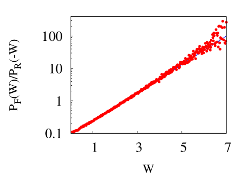
Figure 3: The ratio $P_{F}(W)/P_{R}(-W)$ is plotted versus work $W$ in semi-Log scale and fitted with $\exp[\beta(W-\Delta F)]$ for $L=100$, $\beta=1.0$, $\lambda_{0}=1.0$, $\lambda_{\tau}=11.0$ where $\tau=100$ and $\Delta F=(1/\beta)\ln(\lambda_{\tau}/\lambda_{0})$.

IV.2 Nonconservative force

When a nonconservative force is present in the CS, e.g., a system of particles in a ring in contact with a heat bath and with a force acting in anti-clockwise direction as in Fig. 1, the force field cannot be derived from the gradient of a scalar potential and therefore cannot be absorbed in the expression of the total energy of the CS (e.g., see Eq. 5). In this case, unlike changing an external parameter $\lambda$, the system is driven by changing ${\bf Y}\rightarrow{\bf Y}+\delta{\bf Y}$ as discussed in section III. To illustrate this, we consider a CS which consists of $L+1$ lattice sites in one dimension. The site $i=0$ has energy $e_{0}=p^{2}$, with an internal variable $p$, and any other site $i$ has energy $e_{i}\geq 0$. The site $i=0$ is considered to be the system and the rest is the heat bath. A configuration of the CS is specified by ${\bf Y}\equiv\{p,e_{1},\dots,e_{L}\}$ where, for any given ${\bf Y}$, there is a $\bar{\bf Y}\equiv\{-p,e_{1},\dots,e_{L}\}$. The dynamics is chosen as follows. For $1\leq i\leq L$ we choose a site at random and exchange energy between sites $i$ and $i+1$ randomly,

$$e_{i}\rightarrow q(e_{i}+e_{i+1});\mbox{~{}~{}}e_{i+1}\rightarrow(1-q)(e_{i}+e_{i+1}),$$ (23)

where $q\in[0,1]$ is a uniform random number. The total energy $E=\sum_{i=0}^{L}$ is constant in this process. We update the site $i=0$ slightly differently where we consider that the site $i=0$ can interchange energy only with site $i=1$. Say, energy of the two sites, before update, are $e_{0}=p^{2}$ and $e_{1}$ respectively. We generate a random number $\xi$ uniformly distributed in the range $[-p_{max},p_{max}]$ where $p_{max}=\sqrt{e_{0}+e_{1}}$. We then update the internal variable $p$ and energy of the site $i=0,1$ as given below,

$$p\rightarrow\xi;\mbox{~{}~{}}e_{0}\rightarrow\xi^{2};\mbox{~{}~{}}e_{1}\rightarrow(e_{0}+e_{1}-\xi^{2}).$$ (24)

The update rule ensures that detailed balance is satisfied with respect to a uniform measure on a constant energy surface of the CS. Consequently, while the CS is not driven, the site $i=0$ has the Boltzmann probability distribution $P(p)=\exp(-\beta p^{2})/{\cal Z}$ where $\beta=[\sum_{i=0}^{L}e_{i}/(L+1)]^{-1}$ is inverse temperature of the CS and ${\cal Z}=\int_{-\infty}^{\infty}dp\exp(-\beta p^{2})$ is the partition function.

The system is driven by changing the internal variable $p$ as follows: $p\rightarrow p+\delta$ where $\delta>0$ is a constant (choice of the sign of $\delta$ is arbitrary). Now two following steps performed repeatedly: Step.1 - random sequential update of $L$ bonds of the CS using Eq. 23, 24 and Step.2 - update of the site $i=0$ by changing the internal variable from $p$ to $p+\delta$. The second step may be thought of, as if the internal variable $p$ is like momentum of a particle and it is updated due to effect of an external constant nonconservative force $f$ which changes $p$ by a fixed amount $\delta=f.dt$ in a small time interval $dt$. Note that, under the driving, the transition $p\rightarrow p+\delta$ (also $-(p+\delta)\rightarrow-p$) is allowed, but the transition $p+\delta\rightarrow p$ is not allowed. In other words, internal variable $p$ only changes in one direction, i.e., either increases (for $\delta>0$) or decreases (for $\delta<0$), under the driving. Work $\delta W_{t}$ done on the system is the change in energy of the system (i.e., site $i=0$) where $\delta W_{t}=(p+\delta)^{2}-p^{2}=\delta(2p+\delta)$ and total work $W=\sum_{t}\delta W_{t}$.

The dynamics considered above is similar to the Langevin dynamics of a Brownian particle in a thermal environment where an external nonconservative force is acting on the particle. One should note that, given a trajectory $[p(t),\{e_{i}(t)\}]$, one can define time-reversal operation in two ways, i.e., as $t\rightarrow-t$, $[p(t),\{e_{i}(t)\}]\rightarrow[-p(-t),\{e_{i}(-t)\}]$ or $[p(t),\{e_{i}(t)\}]\rightarrow[p(-t),\{e_{i}(-t)\}]$. But only the first way of time-reversal is relevant here because, given a trajectory $[p(t),\{e_{i}(t)\}]$, the trajectory $[p(-t),\{e_{i}(-t)\}]$ is not realizable as $p$ only increases under the driving. However the microscopic reversibility condition in Eq. 16 is satisfied as the transition probabilities have an additional symmetry, $w(p^{\prime},\{{e_{i}}^{\prime}\}|p,\{e_{i}\})=w(-p,\{e_{i}\}|-p^{\prime},\{{e_{i}}^{\prime}\})$, i.e., $w({\bf Y}^{\prime}|{\bf Y})=w(\bar{\bf Y}|\bar{\bf Y}^{\prime})$.

Following the general proof given in section III, one can see that the Crooks theorem is satisfied, $P(W)/P(-W)=\exp(\beta W)$, where the free energy change $\Delta F=0$. Since the forward and reverse protocol of driving is same in the above example, we have used $P_{F}(W)\equiv P_{R}(W)\equiv P(W)$ in the Crooks theorem. For a time-dependent external nonconservative force, the increment $\delta_{t}$ of the internal variable $p$ at a time step $t$ will be $\delta_{t}=f_{t}.dt$, where $f_{t}$ is the force at time step $t$. In this case, the reverse protocol should be $\{f_{-t}\}$ for a given forward protocol $\{f_{t}\}$, and one should distinguish between the work probability distributions $P_{F}(W)$ and $P_{R}(W)$. Then the Crooks theorem can be written in the more general form as $P_{F}(W)/P_{R}(-W)=\exp(\beta W)$.

V Generalization

The fluctuation theorems can be generalized to the cases where a system is in contact with a heat bath with pressure $P$ and (or) chemical potential $\mu$. Let us consider the combined system with total energy $E$, volume $V$ and number of particles $N$ which are globally conserved. Energy, volume and number of particles $\epsilon$, $v$ and $n$ of the system fluctuate due to interaction with the heat bath. Pressure $P$ and chemical potential $\mu$ can be defined, similar to temperature, as given below,

$$\beta P=\frac{\partial S_{B}(E,V,N)}{\partial V},$$ (25)

$$\beta\mu=\frac{\partial S_{B}(E,V,N)}{\partial N}.$$ (26)

Now using the expansion of the heat bath entropy $S_{B}(E-\epsilon,V-v,N-n)=S_{B}(E,V,N)-\beta\epsilon-\beta Pv-\beta\mu n$ in the limit of $\epsilon\ll E$, $v\ll V$ and $n\ll N$, one can rewrite the ratio of the probabilities of microstates at $t=\pm{\cal T}$, as given in Eq. 20, as

$$\frac{P_{st}({\bf Y}_{-{\cal T}},\lambda_{0})}{P_{st}({\bf Y}_{\cal T},\lambda_{\tau})}=e^{\beta({\cal W}_{F}[\{{\bf Y}_{t},\lambda_{t},\vec{B}_{t}\}]-\Delta{\cal G})}$$ (27)

where ${\cal G}(\beta,P,\mu,\lambda)$ the grand potential of the system in equilibrium with a heat bath of inverse temperature $\beta$, pressure $P$ and chemical potential $\mu$, $\lambda$ an external parameter and $\Delta{\cal G}={\cal G}(\lambda_{\tau})-{\cal G}(\lambda_{0})$ with the grand potential ${\cal G}$ defined as

$${\cal G}(\lambda)=-\frac{1}{\beta}\ln\left[\int d\epsilon\int dv\int dne^{-\beta(\epsilon+Pv+\mu n)}e^{S(\epsilon,v,n,\lambda)}\right]$$ (28)

where $S(\epsilon,v,n,\lambda)$ is entropy of the system. Then the Crooks theorem can be written as given below,

$$\frac{P(W;\lambda(t),\vec{B}(t))}{P(-W;\lambda(-t)_{,}-\vec{B}(-t))}=e^{\beta(W-\Delta{\cal G})}$$ (29)

which is obtained by replacing the Helmholtz free energy $F$ in Eq. 21 by the grand potential ${\cal G}$.

VI Summary

In this paper, we have studied the fluctuation theorems for a classical system in contact with a heat bath in the presence of a time-reversal symmetry-breaking field and nonconservative forces, in a deterministic as well as a stochastic set up. We have shown that the fluctuation theorems are valid under the condition that, in the absence of any driving, the system and the heat bath, combined, relax to a state having a uniform probability measure on a constant energy surface. The fluctuation theorems have been proved in a very general setting by using the time-reversal symmetry and the conservation laws, and accordingly defining the intensive thermodynamic variables like temperature, pressure, chemical potential obtained from a microcanonical ensemble. In the deterministic case of Newtonian dynamics, we have first shown that Liouville’s theorem holds even in the presence of a time-dependent external magnetic field and other time-dependent nonconservative forces and then, using Liouville’s theorem, we have proved the Crooks Theorem and the Jarzynski equality in the presence of such forces. In the stochastic case, where the combined system obeys Markovian dynamics, the work fluctuation theorems have been shown to be valid even when the reverse transition probabilities are not equal to the corresponding forward transition probabilities, thus violating detailed balance condition.

VII Acknowledgments

VIII Appendix

For an equilibrium system, detailed balance with respect to a uniform (microcanonical) probability measure is a sufficient condition for all states to be equally probable in the final equilibrium state. Here we formulate a sufficient condition for having equally probable steady states for a nonequilibrium system with finite number of states.

Figure 4: (Color online) Schematic diagram of a network in a configuration space: Configurations are denoted as nodes $C_{1}$, $C_{2}$, $C_{3}$, $\dots$ $C_{8}$. Nodes are connected by various closed loops, each of which is assigned a transition rate. Transition rates assigned to the dotted arrows should be added to get the corresponding total transition rate.

Figure 5: Network with the magnetic field $\vec{B}$: Transition rates assigned to the dotted arrows in Fig. 4 are added to get the actual transition rate (denoted by the thick arrows in this figure). Transition rates in general depend on the magnetic field.

Although we now specifically consider the case where all reverse transition rates to be zero for corresponding nonzero forward transition rates (similar to the example considered in section IV.A), the following discussion can be straightforwardly generalized to cases where a forward and corresponding reverse transition rate both may be nonzero. Also we only consider here the case where there is no velocity-like variables, however the generalization to such cases is straightforward. In Fig. 4, a network in a configuration space is shown schematically. A configuration $C$ is denoted by a node in the graph. Nodes are connected by drawing closed loops, where each loop is assigned a transition rate, e.g., see Fig. 4 where loops are assigned transition rates $w_{1}$, $w_{2}$, $w_{3}$, etc. If two configurations are connected by more than one loop, each assigned with different transition rates, the total transition rate from one configuration to another is given by sum of the transition rates. For example, in Fig 4, the total transition rate from $C_{2}$ to $C_{1}$ is $w(C_{1}|C_{2})=(w_{1}+w_{2}+w_{3})$. Similarly, $w(C_{3}|C_{1})=(w_{1}+w_{2})$, $w(C_{5}|C_{7})=(w_{4}+w_{5}+w_{6})$, etc. The resulting network is shown in Fig. 5. We call this way of assigning a transition rate (or transition probability) to a closed loop of configurations in a graph as loopwise balance. Only constraint for drawing such loops is that all nodes must be connected to each other along some path so that the system is ergodic. Apart from this, loops are otherwise drawn arbitrarily. Note that since the Markov process is ergodic, it has a unique steady state solution. There are several ways to connect nodes satisfying the constraint of having uniform steady state measure and, since the Markov process is ergodic, all configurations always have equal steady state probabilities. To see this, consider the Master equation for the Markov process defined on a network in Fig. 4,

$$\frac{dP(C_{1})}{dt}=-(w_{1}+w_{2}+w_{3}+w_{6})P(C_{1})$$

$$+(w_{1}+w_{2}+w_{3})P(C_{2})+w_{6}P(C_{5}),$$

$$\frac{dP(C_{2})}{dt}=-(w_{1}+w_{2}+w_{3})P(C_{2})$$

$$+w_{1}P(C_{3})+w_{2}P(C_{8})+w_{3}P(C_{4}),$$

$$\dots$$

$$\dots$$

$$\frac{dP(C_{7})}{dt}=-(w_{4}+w_{5}+w_{6})P(C_{7})$$

$$+(w_{5}+w_{6})P(C_{4})+w_{4}P(C_{8}),$$

$$\frac{dP(C_{8})}{dt}=-(w_{2}+w_{4})P(C_{8})$$

$$+(w_{2}+w_{4})P(C_{3}).$$ (30)

From above set of equations it is clear that all steady states have equal probabilities, i.e., $P(C_{1})=P(C_{2})=P(C_{3})=\dots=P(C_{8})=constant$ is the steady state solution of the Master equation. Since the network is ergodic, the steady state is also unique. Therefore loopwise balance is a sufficient condition for having a uniform steady state measure in an ergodic Markov process with finite number of states.

Figure 6: Network with the reverse magnetic field $-\vec{B}$: Reversal of the direction of the magnetic field $\vec{B}$ corresponds to reversal of all transition rates, i.e., interchanging forward and reverse transition rate. The network for the reverse magnetic field $-\vec{B}$ results from the network of Fig. 5 by reversing all the arrows.

If the Markov process, as defined on the network in Fig. 5, is considered to be in the presence of a magnetic field $\vec{B}$, then the Markov process with the reverse magnetic field $-\vec{B}$ is defined on the same network by assigning transition rates from one node to another in the reverse direction, i.e., just by reversing the arrows on a network as done in Fig. 6. Note that the transition rates assigned to loops in general depend on the magnetic field. However the steady state distribution remains uniform and thus independent of the magnetic field, which is the symmetry relation 2 considered in section III. Note that, although the Master equation changes under reversal of the magnetic field, the steady state solution is still unchanged, i.e., all steady states are still equally probable.

References

- (1) D. J. Evans, E. G. D. Cohen and G. P. Morris, Phys. Rev. Lett. 71, 2401 (1993).
- (2) D. J. Evans and D. J. Searles, Phys. Rev. E 50, 1645 (1994).
- (3) G. Gallavotti and E. G. D. Cohen, Phys. Rev. Lett. 74, 2694 (1995).
- (4) C. Bustamante, J. Liphardt and F. Ritort, Phys. Today 58, 43 (2005).
- (5) R. J. Harris and G. M. Schütz, J. Stat. Mech.: Theor. and Exp. P07020 (2007).
- (6) U. Seifert, Eur. Phys. J. B 64, 423 (2008).
- (7) C. Jarzynski, and D. K. Wojcik, Phys. Rev. Lett. 92, 230602 (2004).
- (8) K. Saito, and A. Dhar, Phys. Rev. Lett. 99, 180601 (2007).
- (9) J. Kurchan, J. Phys. A 31, 3719 (1998).
- (10) J. L. Lebowitz and H. Spohn, J. Stat. Phys. 95, 333 (1999).
- (11) T. Hatano and S. Sasa, Phys. Rev. Lett. 86, 3463 (2001).
- (12) C. Maes and K. Netocny, J. Stat. Phys. 110, 269 (2003).
- (13) U. Seifert, Phys. Rev. Lett. 95, 040602 (2005).
- (14) C. Jarzynski, Phys. Rev. Lett. 78, 2690 (1997).
- (15) S. Park and K. Schulten, J. Chem. Phys. 120, 5946 (2004).
- (16) H. Oberhofer, C. Dellago, and P. L. Geissler, J. Phys. Chem. B 109, 6902 (2005).
- (17) G. E. Crooks, Phys. Rev. E 60, 2721 (1999).
- (18) R. A. Blythe, Phys. Rev. Lett. 100, 010601 (2008).
- (19) O. Narayan and A. Dhar, J. Phys. A: Math. Gen. 37, 63 (2004).
- (20) T. Mai and A. Dhar, Phys. Rev. E 75, 061101 (2007).
- (21) T. Speck and U. Seifert, J. Stat. Mech: Theor. and Exp. L09002 (2007).
- (22) G. E. Crooks, Phys. Rev. E 61, 2361 (2000).
- (23) E. G. D. Cohen and D. Mauzerall, J. Stat. Mech: Theor. and Exp. P07006 (2004).
- (24) E. G. D. Cohen and D. Mauzerall, Molecular Physics 103, 2923 (2005).
- (25) E. T. Jaynes, Phys. Rev. 106, 620 (1957). E. T. Jaynes, Phys. Rev. 108, 171 (1957).
- (26) R. M. L. Evans, Phys. Rev. Lett. 92, 150601 (2004).
- (27) R. M. L. Evans, J. Phys. A: Math. Gen. 38, 293 (2005).
- (28) A. Simha, R. M. L. Evans, and A. Baule, Phys. Rev. E 77, 031117 (2008).
- (29) C. Jarzynski, J. Stat. Phys. 98, 77 (2000).
- (30) B. Cleuren, C. Van den Broeck and R. Kawai, Phys. Rev. Lett. 96, 050601 (2006).
- (31) P. Pradhan, Y. Kafri, and D. Levine, Phys. Rev. E 77, 041129 (2008).
- (32) K. Saito and Y. Utsumi, Phys. Rev. B 78, 115429 (2008).
- (33) A. M. Jayannavar and M. Sahoo, Phys. Rev. E 75, 032102 (2007).
- (34) D. Roy and N. Kumar, Phys. Rev. E 78, 052102 (2008).
- (35) A. Saha and A. M. Jayannavar, Phys. Rev. E 77, 022105 (2008).
- (36) R. C. Tolman, The Principles of Statistical Mechanics (Clarendon Press, Oxford, 1938).
- (37) Since some amount of work done on the system gets dissipated to the heat bath, there is a slight change in temperature of the bath (although is infinitesimal due to large size of a bath). The net free energy change of the CS equals where is a finite change in free energy of the bath and is entropy of the bath Narayan .
- (38) H. Goldstein, C. Poole, and J. Safko, Classical Mechanics, (Addison-Wesley, Third Edition, 2000).
- (39) N. G. van Kampen, Stochastic processes in Physics and Chemistry (Amsterdam: Elsevier, 1992), page 114-117.
- (40) S. R. de Groot and P. Mazur, Non-equilibrium Thermodynamics (Dover Publications, New York, 1884), page 92-100.
- (41) J. H. Van Vleck, The Theoty of electric and Magnetic Susceptibilities (The Clarendon Press, Oxford, 1932), page 22, page 97-99.
- (42) M. R. Evans and T. Hanney, J. Phys. A: Math. Gen. 38, R195 (2005).