Visible parts of fractal percolation

Abstract.

We study dimensional properties of visible parts of fractal percolation in the plane. Provided that the dimension of the fractal percolation is at least 1, we show that, conditioned on non-extinction, almost surely all visible parts from lines are 1-dimensional. Furthermore, almost all of them have positive and finite Hausdorff measure. We also verify analogous results for visible parts from points. These results are motivated by an open problem on the dimensions of visible parts, see [M2].

1. Introduction, notation and results

1.1. Visible parts

The visible part of a compact set $E\subset\mathbb{R}^{2}$ from an affine line $\ell$ consists of those points $x\in E$ where one first hits the set $E$ when looking perpendicularly from $\ell$. More precisely:

Definition 1.1.

Let $E\subset\mathbb{R}^{2}$ be compact and let $\ell$ be an affine line not meeting $E$. The visible part $V_{\ell}(E)$ of $E$ from $\ell$ is

$$V_{\ell}(E)=\{a\in E:[a,\Pi_{\ell}(a)]\cap E=\{a\}\}$$

where $\Pi_{\ell}(a)$ is the projection of $a$ onto $\ell$ and $[a,\Pi_{\ell}(a)]$ is the closed line segment joining $a$ to $\Pi_{\ell}(a)$. Moreover, the visible part $V_{x}(E)$ of $E$ from a point $x\in\mathbb{R}^{2}\setminus E$ is

$$V_{x}(E)=\{a\in E:[a,x]\cap E=\{a\}\}.$$

In this paper we restrict our consideration to the planar case. Clearly, Definition 1.1 can be extended in a natural way to higher dimensions, see [JJMO]. For a measure theoretic definition of visibility and related topics, see [Cs] and [M2].

The question of how the Hausdorff dimension, $\operatorname{dim_{H}}$, of visible parts depends on that of the original set has been considered in [JJMO] and [O]. In general, only “almost all” type of results are possible since there may be exceptional directions, for example in the case of fractal graphs, see [JJMO]. Let $\mathcal{L}^{n}$ be the Lebesgue measure on $\mathbb{R}^{n}$. There is a natural Radon measure $\Gamma$ on the space $\mathcal{A}$ of affine lines in the plane, that is, for all $A\subset\mathcal{A}$

$$\Gamma(A)=\int\mathcal{L}^{1}(\{a\in L^{\perp}:L+a\in A\})\,d\gamma(L),$$

where $L$ is a line that goes through the origin, $L^{\perp}$ is the orthogonal complement of $L$ and $\gamma$ is the natural Radon measure on the space of all lines that go through the origin. Since every line through the origin can be parametrised by the angle which it makes with the positive $x$-axis, the Lebesgue measure $\mathcal{L}^{1}$ on the half open interval $[0,\pi)$ induces $\gamma$.

Let $E\subset\mathbb{R}^{2}$ be a compact set. The results in [JJMO] for dimensional properties of visible parts resemble the Marstrand-Kaufman-Mattila -type projection results, according to which

(1.1) $$\operatorname{dim_{H}}\Pi_{L}(E)=\min\{\operatorname{dim_{H}}E,1\}$$

for $\gamma$-almost all lines $L$ that go through the origin [M1]. For visible parts we have: if $\operatorname{dim_{H}}E\leq 1$ then

(1.2) $$\operatorname{dim_{H}}V_{\ell}(E)=\operatorname{dim_{H}}E\text{ and }\operatorname{dim_{H}}V_{x}(E)=\operatorname{dim_{H}}E$$

for $\Gamma$-almost all affine lines $\ell$ not meeting $E$ and for $\mathcal{L}^{2}$-almost all $x\in\mathbb{R}^{2}\setminus E$. On the other hand, if $\operatorname{dim_{H}}E>1$, then

(1.3) $$1\leq\operatorname{dim_{H}}V_{\ell}(E)\text{ and }1\leq\operatorname{dim_{H}}V_{x}(E)$$

for $\Gamma$-almost all affine lines $\ell$ not meeting $E$ and for $\mathcal{L}^{2}$-almost all $x\in\mathbb{R}^{2}\setminus E$. These results can be extended to higher dimensions by replacing 1 with $n-1$, see [JJMO].

The methods utilised in [JJMO] for proving (1.2) and (1.3) are based on the generalized projection formalism for parametrised families of transversal mappings due to Y. Peres and W. Schlag [PS]. The asymmetry between (1.1) and (1.3) in the case $\operatorname{dim_{H}}E>1$ is due to the following: in (1.1) the upper bound $\operatorname{dim_{H}}\Pi_{L}(E)\leq 1$ is trivial since $\Pi_{L}(E)$ is a subset of a line. However, $V_{\ell}(E)$ does not have this restriction and a priori its dimension could be as large as the dimension of $E$ (and indeed this can be the case, at least for exceptional lines, as in the already mentioned example of fractal graphs.)

The validity of the reverse inequality of (1.3) in general is an open problem. In [JJMO] it was verified for some concrete examples, including quasi-circles and certain self-similar sets. In the planar case a partial answer was given by T. C. O’Neil in [O]. Using energies, he showed that if a compact connected plane set $E$ has Hausdorff dimension strictly larger than one, then visible parts from almost all points have Hausdorff dimension strictly less than the Hausdorff dimension of $E$. In fact, for $\mathcal{L}^{2}$-almost all $x\in\mathbb{R}^{2}\setminus E$,

$$\operatorname{dim_{H}}V_{x}(E)\leq\frac{1}{2}+\sqrt{\operatorname{dim_{H}}E-\frac{3}{4}}.$$

It is easy to see that $1$ is the only possible universal value for Hausdorff dimension of typical visible parts of sets $E$ with $\operatorname{dim_{H}}E>1$. More precisely, if for all compact sets $E\subset\mathbb{R}^{2}$ with $\operatorname{dim_{H}}E>1$ there exists a constant $c$ such that $\operatorname{dim_{H}}V_{\ell}(E)=c$ for almost all $\ell$, then $c=1$, see [JJMO]. In this paper we verify that this constancy result holds, in a strong form, for typical random sets in fractal percolation.

1.2. Fractal percolation

Fractal percolation is a natural model of fractal sets that display stochastic self-similarity. Much is known about its geometric properties, see [C] and [G] and the references therein. We address the question of studying dimensional properties of visible parts of fractal percolation in the plane. It turns out that the reverse inequality in (1.3) holds for all lines almost surely conditioned on non-extinction, in a strong quantitative form. Moreover, the visible parts from almost every line have positive and finite 1-dimensional Hausdorff measure. We underline that the methods we use are different from those in [JJMO] and [O]. Before stating the results, we recall the construction of fractal percolation and discuss some of its basic properties.

Fix $0<p<1$. We construct a random compact set as follows: Let $Q_{0}=[0,1]\times[0,1]\subset\mathbb{R}^{2}$ be the unit square. Divide $Q_{0}$ into four subsquares of equal size each of which is chosen with probability $p$ and dropped with probability $1-p$, independently of each other. Denote by $\mathcal{C}_{1}$ the collection of all chosen subsquares. For each $Q\in\mathcal{C}_{1}$, we continue the same process by dividing $Q$ into four subsquares of equal size. Again each of these subsquares is chosen with probability $p$ and dropped with probability $1-p$, independently of each other. The set of all chosen squares at the second level is denoted by $\mathcal{C}_{2}$. Repeating this process inductively gives the limiting random set $E$, defined as

$$E=\bigcap_{n=1}^{\infty}\bigcup\{Q:Q\in\mathcal{C}_{n}\}.$$

The probability space $\Omega$ is the space of all constructions and the natural probability measure on $\Omega$ induced by this procedure is denoted by $\mathbf{P}$.

In [CCD] J.T. Chayes, L. Chayes and R. Durrett verified that there is a critical probability $0<p_{c}<1$ such that if $p<p_{c}$, then with probability one $E$ is totally disconnected, whereas the opposing sides of $Q_{0}$ are connected with positive probability provided that $p>p_{c}$. This phenomenon is commonly referred to as fractal percolation.

We review some of the most basic facts on fractal percolation, and refer the reader to [G] or to [C] for further background. Clearly, if $p<1$, then there is a positive probability that the limit set $E$ is empty. A more subtle question is for which values of $p$ the set $E$ is empty almost surely. It turns out that

$$\mathbf{P}(E=\emptyset)=1\text{ if and only if }p\leq\frac{1}{4}.$$

Moreover, conditioned on non-extinction, that is $E\neq\emptyset$, we have

$$\operatorname{dim_{H}}E=\frac{\log(4p)}{\log 2}$$

almost surely. This implies that, conditioned on non-extinction, $\operatorname{dim_{H}}E>1$ almost surely provided that $p>\frac{1}{2}$. In particular, when considering dimensional properties of visible parts of $E$, we may restrict our consideration to the case $p>\frac{1}{2}$, as the case $\frac{1}{4}<p\leq\frac{1}{2}$ is covered by the general equation (1.2).

Remark 1.2.

Instead of working with base 2 in the definition of fractal percolation one could work with base $M$ for $M\geq 2$, i.e. divide each square into $M^{2}$ subsquares of equal size and choose each of them with probability $p$ and drop with probability $1-p$, independently of each other. It is straightforward to see that all the results of this paper remain true also in this case (with the threshold $p=\frac{1}{2}$ replaced by $p=\frac{1}{M}$). For notational simplicity we restrict our consideration to the case $M=2$.

1.3. Statement of results

For a positive integer $k$, let $N_{k}(A)$ be the number of dyadic squares of side length $2^{-k}$ that intersect a set $A\subset\mathbb{R}^{2}$. Recall that the upper box dimension of a compact set $A$ is given by

$$\overline{\dim}_{B}A=\limsup_{k\to\infty}\frac{\log N_{k}(A)}{\log 2^{k}}.$$

Likewise one defines lower box dimension, and one says that the box dimension exists, and is denoted by $\dim_{B}A$, if the lower and upper versions coincide. We denote the 1-dimensional Hausdorff measure by $\mathcal{H}^{1}$. We now state our main results.

Theorem 1.3.

Let $p>\frac{1}{2}$. Conditioned on non-extinction, almost surely

$$\operatorname{dim_{H}}V_{\ell}(E)=\operatorname{dim_{B}}V_{\ell}(E)=1$$

for all lines $\ell$ not meeting $E$. Moreover, for any sequence $\{a_{k}\}$ such that $\frac{a_{k}}{k}\rightarrow\infty$, one has almost surely that

(1.4) $$N_{k}(V_{\ell}(E))\leq a_{k}2^{k}$$

simultaneously for all lines $\ell$ not meeting $E$ for all $k\geq K$. Here $K$ depends on $E$, $\ell$ and the sequence $a_{k}$.

Remark 1.4.

For any closed $D\subset S^{1}$ with $D\cap\{(\pm 1,0),(0,\pm 1)\}=\emptyset$ one can choose uniform $K$ in (1.4) for all $\ell$ with $\ell\cap Q_{0}=\emptyset$ and $\theta(\ell)\in D$, where $\theta(\ell)$ is the angle between $\ell^{\perp}$ and the $x$-axis.

We are also able to show that visible parts from a given line typically have positive and finite length:

Theorem 1.5.

Let $\ell$ be any fixed line. Assume that $p>\frac{1}{2}$. Then

$$0<\mathcal{H}^{1}(V_{\ell}(E))<\infty$$

almost surely conditioned on non-extinction and $E\cap\ell\neq\emptyset$.

As an immediate consequence of Theorem 1.5 we have:

Corollary 1.6.

Let $p>\frac{1}{2}$. Conditioned on non-extinction, almost surely

$$0<\mathcal{H}^{1}(V_{\ell}(E))<\infty$$

for almost all lines $\ell$ which do not meet the unit square.

We do not know whether the exceptional set $\{E:\mathcal{H}^{1}(V_{\ell}(E))=\infty\}$ in Theorem 1.5 depends on $\ell$.

Above results concern visible parts from lines. Similar results are available for visible parts from points; see Theorems 4.2 and 4.3 in Section 4.

1.4. Notation and organization

We henceforth fix a value of $p\in(\frac{1}{2},1)$ for the rest of the paper. We will use the $O(\cdot),\Omega(\cdot)$ notation: if $x,y$ are two positive quantities, by $x=O(y)$ we mean that $x\leq Cy$ for some constant $C$, and by $x=\Omega(y)$ we mean $y=O(x)$. The implicit constant may depend only on $p$. In particular, if the quantities $x,y$ are related to a stage $n$ of the construction of fractal percolation, then the implicit constant is independent of $n$.

The paper is organized in the following manner: in the next section we verify crucial technical lemmas, in Section 3 we prove our main theorems concerning visible parts from lines, and in the last section we study visible parts from points.

2. Technical lemmas

In this section we verify some lemmas needed in the proof of our main theorems. We start by showing that in Theorems 1.3 and 1.5 it is enough to consider lines that do not meet the closed unit square $Q_{0}$. For all positive integers $n$, we will denote the set of all dyadic subsquares of $Q_{0}$ of side length $2^{-n}$ by $\mathcal{Q}_{n}$. Recall that $\mathcal{C}_{n}$ is the random subset of $\mathcal{Q}_{n}$ consisting of the chosen squares of side length $2^{-n}$. Throughout the paper, by a square we mean a closed dyadic square with sides parallel to the axes.

Lemma 2.1.

In Theorem 1.3, it is enough to prove the statement for all lines not meeting $Q_{0}$. Likewise, in Theorem 1.5 one may assume that $\ell\cap Q_{0}=\emptyset$ (in which case $\ell\cap E=\emptyset$ automatically and one does not need to condition on this.)

Proof.

We present the argument for Theorem 1.3; for Theorem 1.5 it is analogous.

Assume that (1.4) holds for all lines not meeting $Q_{0}$ and fix a sequence $a_{k}$ with $\frac{a_{k}}{k}\rightarrow\infty$. Given a dyadic square $Q\in\mathcal{Q}_{n}$, let $A_{Q}$ be the event “for every line $\ell$ not meeting $Q$, the visible part $V_{\ell}(E\cap Q)$ can be covered by $4^{-n}a_{k}2^{k}$ dyadic squares of side-length $2^{-k}$, for all large enough $k$”. By our assumption for the sequence $4^{-n}a_{k}$ and the self-similarity of $E$, each $A_{Q}$ has full probability, and so does the event

$$A=\bigcap_{n=1}^{\infty}\bigcap_{Q\in\mathcal{Q}_{n}}A_{Q}.$$

On the other hand, a line $\ell$ does not meet $E$ if and only if there is $n$ such that $\ell$ does not meet any square in $\mathcal{C}_{n}$. Clearly, if $\ell$ is such a line, then

$$V_{\ell}(E)\subset\bigcup_{Q\in\mathcal{C}_{n}}V_{\ell}(Q\cap E).$$

This inclusion shows that (1.4) holds whenever $A$ holds, and thus it is an almost sure event.

The assertions on the Hausdorff and box dimensions follow easily from (1.4); see the proof of Theorem 1.3. ∎

In the light of the previous lemma, we may assume that the line $\ell$ does not meet $Q_{0}$. Horizontal and vertical lines are exceptional, and are easier to handle; see [J] for the proof of Theorem 1.5 in this case (a slightly weaker version of Theorem 1.3 is also proved there; the full version follows using the large deviation ideas used in this article). Therefore from now on we will focus on the transversal case. We assume that $\ell$ is of the form $y=-tx-a$, where $t,a>0$, since the other cases follow by symmetry. Such a line will be fixed for the rest of this section.

Given $0<\varepsilon<\frac{1}{2}$, we associate a set $Q(\varepsilon)$ to each square $Q$ of side length $a$ as follows: $Q(\varepsilon)$ is obtained by removing from $Q$ the half-open squares of side length $\varepsilon a$ from the upper left and the lower right corners, see Figure 3. (For lines of positive slope, one would need to remove the lower left and the upper right corners.)

The following theorem from [RS] will play a crucial role in our study. Recall that $Q_{0}$ denotes the closed unit square.

Theorem 2.2.

Let $D\subset S^{1}$ be a closed connected arc such that

$$D\cap\{(\pm 1,0),(0,\pm 1)\}=\emptyset.$$

Then for any $0<\varepsilon<\frac{1}{2}$ there exists $q_{\varepsilon}>0$ such that

$$\mathbf{P}(\Pi_{\ell}(E)\supset\Pi_{\ell}(Q_{0}(\varepsilon))\text{ for all }\ell\text{ with }\theta(\ell)\in D)=q_{\varepsilon}.$$

Here $\theta(\ell)$ is the angle between $\ell^{\perp}$ and the $x$-axis.

Proof.

Thhis is proved in [RS]. For the convenience of the reader, a proof is also sketched in the proof of Lemma 4.5. ∎

Given $Q\in\mathcal{Q}_{n}$, where $n\geq 3$, let $\widetilde{Q}\in\mathcal{Q}_{n-2}$ be the unique dyadic square which contains $Q$. We say that a square $Q$ is a corner if the relative position of $Q$ within $\widetilde{Q}$ is either the upper left corner or the lower right one.

Let $0<\varepsilon<\frac{1}{3}$ and let $n\geq 3$ be an integer. Denote the centre of a square $Q$ by $z(Q)$. Given an interval $I\subset\Pi_{\ell}(Q_{0})$ of length $\varepsilon 2^{-n}$, we consider the collections

$$\mathcal{Q}_{I}=\{Q\in\mathcal{Q}_{n}:\Pi_{\ell}(z(Q))\in I\}$$

and

$$\mathcal{C}_{I}=\mathcal{Q}_{I}\cap\mathcal{C}_{n}.$$

The interval $I$ will be fixed for the moment. Write

$$\mathcal{Q}_{I}=\{Q_{1},\ldots,Q_{M}\},$$

where $\operatorname{dist}(z(Q_{i}),\ell)<\operatorname{dist}(z(Q_{i+1}),\ell)$ for $i=1,\ldots,M-1$. Here $\operatorname{dist}(x,A)=\inf\{|x-a|:a\in A\}$ is the distance between a point $x$ and a set $A$. Likewise, set

$$\mathcal{C}_{I}=\{C_{1},\ldots,C_{N}\},$$

where $\operatorname{dist}(z(C_{i}),\ell)<\operatorname{dist}(z(C_{i+1}),\ell)$ for $i=1,\ldots,N-1$. Both $C_{i}$ and $N$ are random variables, while $Q_{i}$ and $M$ are deterministic, but depend on the interval $I$.

Let $Z_{i}$ be the indicator function for the event “$C_{i}$ is a corner” with the interpretation that $Z_{i}=0$ if $i>N$. Define

$$X_{m}=\sum_{i=1}^{m}Z_{i}.$$

Furthermore, let $\mathcal{X}_{m}$ be the algebra generated by $X_{1},\ldots,X_{m}$(or by $Z_{1},\ldots,Z_{m}$). The following technical lemma will be a crucial tool in the proofs. It asserts that, whatever the distribution of corners and non-corners among $C_{1},\ldots C_{m-1}$ is, there is a uniformly positive probability that the next chosen square $C_{m}$ (if defined) is not a corner.

Lemma 2.3.

There exists $\zeta<1$ depending only on $p$ (and not on $n$, $m$ or the interval $I$) such that

(2.1) $$\mathbf{P}(Z_{m}=1\mid\mathcal{X}_{m-1})\leq\zeta.$$

We start by establishing three claims that will be useful in the proof of the lemma.

Claim 1. For any $i\in\{1,\ldots,M-2\}$, at least one of the successive squares $Q_{i},Q_{i+1},Q_{i+2}\in\mathcal{Q}_{I}$ is not a corner.

Proof of Claim 1.

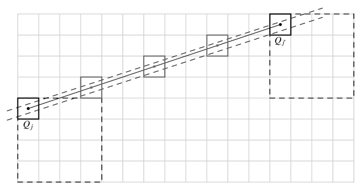
Figure 1. The proof of Claim 1: the solid segment joining the centres of $Q_{j}$ and $Q_{j^{\prime}}$ is $J$, and the parallel dashed lines represent the boundary of the stripe $S$. A square is in $\mathcal{Q}_{I}$ if its centre lies on this stripe. If $Q_{j},Q_{j^{\prime}}$ are in $\mathcal{Q}_{I}$ and are both corners of the same type, then we can find three other squares between them with centres in $J$, which are therefore also in $\mathcal{Q}_{I}$.

Suppose that $Q_{i},Q_{i+1},Q_{i+2}$ are all corners. Then there are $j<j^{\prime}\in\{i,i+1,i+2\}$ such that $Q_{j}$ and $Q_{j^{\prime}}$ are corners of the same type, i.e. both of them are either upper left or lower right corners. By definition of $\mathcal{Q}_{I}$, $z(Q_{j})$ and $z(Q_{j^{\prime}})$ both lie in the stripe $S$ of lines through $I$ orthogonal to $\ell$; see Figure 1. Let $J$ denote the segment that joins $z(Q_{j})$ and $z(Q_{j^{\prime}})$, and denote its length by $|J|$. By elementary algebra, the points on $J$ at distance $\frac{1}{4}|J|$, $\frac{1}{2}|J|$ and $\frac{3}{4}|J|$ from $z(Q_{j})$ are all centres of squares in $\mathcal{Q}_{n}$. Since $J$ is contained in $S$, this implies that these three squares are in fact in $\mathcal{Q}_{I}$. Hence $j^{\prime}-j\geq 4$, which is a contradiction since we had assumed that $j^{\prime}-j\in\{1,2\}$. ∎

Claim 2. Let $Q$, $\widehat{Q}\in\mathcal{Q}_{I}$ be successive squares with $\operatorname{dist}(z(Q),\ell)<\operatorname{dist}(z(\widehat{Q}),\ell)$. Then

$$\mathbf{P}(\widehat{Q}=C_{1})\geq(1-p)\mathbf{P}(Q=C_{1}).$$

Proof of claim 2.

Let $R$ be the smallest dyadic square containing both $Q$ and $\widehat{Q}$, and let $R_{Q}$ and $R_{\widehat{Q}}$ be the largest dyadic proper subsquares of $R$ containing $Q$ and $\widehat{Q}$, respectively. Then $R_{Q}\neq R_{\widehat{Q}}$. Denote by $A$ the event “$R$ is chosen and there are no chosen squares in $\mathcal{Q}_{I}$ which are closer to $\ell$ than those inside $R$”. As “$Q=C_{1}$” and “$\widehat{Q}=C_{1}$” are subevents of $A$, it is enough to prove that

$$\mathbf{P}(\widehat{Q}=C_{1}\mid A)\geq(1-p)\mathbf{P}(Q=C_{1}\mid A).$$

Since $Q=C_{1}$ in particular implies that $Q$ is chosen, we have

$$\mathbf{P}(Q=C_{1}\mid A)\leq\mathbf{P}(Q\in\mathcal{C}_{I}\mid A)=\mathbf{P}(\widehat{Q}\in\mathcal{C}_{I}\mid A).$$

Conditioned on $A$, the event “$\widehat{Q}\in\mathcal{C}_{I}$ and $R_{Q}$ is not chosen” is a subevent of “$\widehat{Q}=C_{1}$”, and moreover, the events “$\widehat{Q}\in\mathcal{C}_{I}$” and “$R_{Q}$ is not chosen” are independent conditioned on $R$ being chosen. This implies

$$\mathbf{P}(\widehat{Q}=C_{1}\mid A) \geq\mathbf{P}(\widehat{Q}\in\mathcal{C}_{I}\text{ and }R_{Q}\text{ is not chosen}\mid A)$$

$$=\mathbf{P}(\widehat{Q}\in\mathcal{C}_{I}\mid A)\mathbf{P}(R_{Q}\text{ is not chosen}\mid A)$$

$$\geq(1-p)\mathbf{P}(Q=C_{1}\mid A).$$

∎

Claim 3. Suppose that at least one square in $\mathcal{Q}_{n}$ is not a corner. Then

(2.2) $$\mathbf{P}(Z_{1}=0\mid\mathcal{C}_{I}\neq\emptyset)=\Omega(1).$$

Proof of claim 3.

Denote the collection of corners by $\operatorname{Cor}$. We may write $\operatorname{Cor}=\operatorname{Cor}_{1}\cup\operatorname{Cor}_{2}\cup\operatorname{Cor}_{3}$ where, for $i\leq M-2$, the square $Q_{i}\in\operatorname{Cor}_{1}$ if $Q_{i+1}\notin\operatorname{Cor}$ and $Q_{i}\in\operatorname{Cor}_{2}$ provided that $Q_{i+1}\in\operatorname{Cor}$, and $\operatorname{Cor}_{3}=\operatorname{Cor}\cap\{Q_{M-1},Q_{M}\}$.

According to Claim 1, for $j=1,2$ we may attach to any square $Q_{i}\in\operatorname{Cor}_{j}$ the square $Q_{i+j}\notin\operatorname{Cor}$. Thus for any $Q_{i}\in\operatorname{Cor}_{j}$ ($j=1,2$) the events “$Q_{i}=C_{1}$” and “$Q_{i+j}=C_{1}$” are subevents of “$\mathcal{C}_{I}\neq\emptyset$ and $C_{1}\notin\operatorname{Cor}_{3}$”. Write $A$ for the latter event. By Claim 2 we obtain that

$$\mathbf{P}(Q_{i+j}=C_{1}\mid A)\geq(1-p)^{j}\mathbf{P}(Q_{i}=C_{1}\mid A).$$

Hence, using that $C_{1}\notin\operatorname{Cor}_{3}$,

$$1= \left(\sum_{Q\in\operatorname{Cor}_{1}}+\sum_{Q\in\operatorname{Cor}_{2}}+\sum_{Q\notin\operatorname{Cor}}\right)\mathbf{P}(Q=C_{1}\mid A)$$

$$\leq \left(\frac{1}{(1-p)^{2}}+\frac{1}{1-p}+1\right)\sum_{Q\notin\operatorname{Cor}}\mathbf{P}(Q=C_{1}\mid A),$$

implying that $\mathbf{P}(Z_{1}=0\mid A)=\Omega(1)$.

Since every $Q\in\mathcal{Q}_{I}$ has the same probability of being chosen, we have $\mathbf{P}(Q_{1}=C_{1})\geq\mathbf{P}(Q_{i}=C_{1})$ for all $i=2,\dots,M$, giving $\mathbf{P}(C_{I}\neq\emptyset)\leq 3\mathbf{P}(A)$. Hence

$$\mathbf{P}(Z_{1}=0\mid C_{I}\neq\emptyset) \geq\mathbf{P}(Z_{1}=0\textrm{ and }C_{1}\notin\operatorname{Cor}_{3}\mid C_{I}\neq\emptyset)$$

$$\geq\frac{1}{3}\mathbf{P}(Z_{1}=0\mid A)=\Omega(1).$$

This gives (2.2). ∎

Now we are ready to prove Lemma 2.3.

Proof of Lemma 2.3.

Let $\mathcal{Y}_{m}$ be the algebra generated by the random variables $C_{1},\ldots,C_{m\wedge N}$ and the event “$m\leq N$”. Note that this is a refinement of $\mathcal{X}_{m}$. Hence it is enough to prove that

(2.3) $$\mathbf{P}(Z_{m}=1\mid\mathcal{Y}_{m-1})=1-\Omega(1).$$

We assume $m\leq N$; otherwise there is nothing to prove. Let $i_{0}$ be the index for which $C_{m-1}=Q_{i_{0}}$. Note that $i_{0}<M$, since otherwise $m-1=N$.

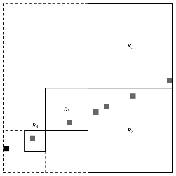
Figure 2. Construction of the rectangles $R_{i}$: the black square represents $C_{m-1}$, and the gray squares are the remaining squares in $\mathcal{Q}_{I}$ after $C_{m-1}$.

We select a finite collection $\{R_{i}\}$ of dyadic squares inductively in the following manner: Let $R_{1}$ be the largest dyadic square which contains $Q_{M}$ but does not contain $C_{m-1}$. Assuming that dyadic squares $R_{1},\dots,R_{i}$ have been selected, pick the largest index $i_{0}<j<M$ such that $Q_{j}$ is not contained in $R_{1}\cup\dots\cup R_{i}$. Let $R_{i+1}$ be the largest dyadic square which contains $Q_{j}$ but does not contain $C_{m-1}$. The process stops when we have a collection $\{R_{1},\dots,R_{L}\}$ such that for all $i_{0}<j\leq M$ the square $Q_{j}$ belongs to $R_{i}$ for some unique $i=1,\dots,L$. See Figure 2.

By construction, $C_{m-1}$ belongs to the dyadic square containing $R_{i}$ and having side length twice of that of $R_{i}$ (see Figure 2; these squares are represented by dotted lines). Therefore, the side length of $R_{i+1}$ is at most that of $R_{i}$ for all $i=1,\dots,L-1$, and each $R_{i}$ has probability $p$ of being chosen, independently of each other.

Assume first that all the squares after $C_{m-1}$ in $\mathcal{Q}_{I}$ are corners. Then, by Claim 1, there are at most two of them, which gives $L\leq 2$. Thus the probability that neither of the two corners in $\mathcal{Q}_{I}$ after $\mathcal{C}_{m-1}$ is chosen is at least $(1-p)^{2}$, giving

$$\mathbf{P}(Z_{m}=1\mid\mathcal{Y}_{m-1})\leq 1-(1-p)^{2}.$$

Now assume that there is $R_{i}$ containing at least one square in $\mathcal{Q}_{I}$ which is not in $\operatorname{Cor}$. To see that (2.3) holds, divide the collection $\{R_{1},\dots,R_{L}\}$ into two parts $P_{\textrm{bad}}$ and $P_{\textrm{good}}$ as follows: we say that $R_{i}\in P_{\textrm{bad}}$ if all squares that belong to $\mathcal{Q}_{I}$ and are contained in $R_{i}$ are corners, and $R_{i}\in P_{\textrm{good}}$ if $R_{i}$ contains a square that belongs to $\mathcal{Q}_{I}$ and is not a corner.

Since each $R_{i}$ contains some square in $\mathcal{Q}_{I}$, we may use Claim 1 as in the proof of Claim 3 to find that we may attach to any $R_{i}\in P_{\textrm{bad}}$, with $i\leq L-2$, a square $R_{i+j}\in P_{\textrm{good}}$ where $j=1$ or $2$. The same argument of Claim 3 then gives

$$\mathbf{P}(C_{m}\subset R_{i}\textrm{ for some }R_{i}\in P_{\textrm{good}}\mid\mathcal{Y}_{m-1})=\Omega(1).$$

(Recall that we are conditioning on $P_{\textrm{good}}$ being non-empty.) Hence it remains to prove that

$$\mathbf{P}(Z_{m}=0|C_{m}\subset R_{i}\textrm{ for some }R_{i}\in P_{\textrm{good}},\mathcal{Y}_{m-1})=\Omega(1).$$

However, by conditioning on the index $i$ for which $C_{m}\subset R_{i}$, we are exactly in the situation of Claim 3 (applied to some $n^{\prime}<n$ and a different interval $I^{\prime}$).

This completes the proof of the lemma. ∎

As a corollary, we obtain the following large deviation bound for $X_{m}$:

Lemma 2.4 (Azuma-Hoeffding inequality).

Let $\zeta$ be as in Lemma 2.3 and choose $\eta>0$ such that $\zeta+\eta<1$. Then

$$\mathbf{P}(X_{m}>(\zeta+\eta)m)<e^{-\frac{\eta^{2}m}{2}}.$$

Proof.

Define $Y_{i}=Z_{i}-\zeta$ and $\widetilde{X}_{m}=\sum_{i=1}^{m}Y_{i}$. Then $\widetilde{X}_{m}$ is a (discrete time) supermartingale, that is, $\mathbf{E}(\widetilde{X}_{m}\mid\widetilde{X}_{1},\dots,\widetilde{X}_{m-1})\leq\widetilde{X}_{m-1}$. Applying the Azuma-Hoeffding inequality [ASE, Theorem 7.2.1] to $\widetilde{X}_{m}$ with $\lambda=\eta\sqrt{m}$ gives the claim. Note that [ASE, Theorem 7.2.1] is verified only for martingales but the same proof works for supermartingales as well. ∎

3. Visible parts from lines

This section is dedicated to the proofs of Theorems 1.3 and 1.5, and Corollary 1.6. We start with Theorem 1.5 for clarity of exposition, as the proof is somewhat easier than that of Theorem 1.3.

Proof of Theorem 1.5.

As remarked in the previous section, it is enough to prove the theorem for a fixed line $\ell=-tx-a$ with $t,a>0$. By Theorem 2.2, $\mathcal{H}^{1}(V_{\ell}(E))>0$ almost surely conditioned on non-extinction, and therefore we only need to prove that

$$\mathcal{H}^{1}(V_{\ell}(E))<\infty$$

almost surely.

Denote by $\theta$ the angle between $\ell^{\perp}$ and the positive $x$-axis, and let $\varepsilon<\tfrac{1}{2}\sin\theta\cos\theta$. (The factor $\sin\theta$ is needed when $\theta$ is close to 0 and the factor $\cos\theta$ is essential when $\theta$ is close to $\frac{\pi}{2}$.) Given a positive integer $n$, let $N(n)$ be the smallest integer such that $N(n)\varepsilon 2^{-n}\geq\sqrt{2}$. Then $N(n)\leq 2\varepsilon^{-1}2^{n}$. Divide $\Pi_{\ell}(Q_{0})$ into disjoint line segments of length $\varepsilon 2^{-n}$ (except for the last one which may be smaller), and denote them by $I_{n,1},\ldots,I_{n,N(n)}$. For all $1\leq j\leq N(n)$, set $\mathcal{Q}_{n,j}=\mathcal{Q}_{I_{n,j}}$.

We say that $Q\in\mathcal{Q}_{n,j}$ induces a block if $Q$ is not a corner and the unique square $\widetilde{Q}\in\mathcal{Q}_{n-2}$ which contains $Q$ is a block, meaning that

$$\Pi_{\ell}(\widetilde{Q}(\frac{1}{8}))\subset\Pi_{\ell}(\widetilde{Q}\cap E).$$

If $Q$ is not a corner and $\widetilde{Q}$ is not a block, we say that $\widetilde{Q}$ is a window and $Q$ induces a window. By Theorem 2.2 and independence, every chosen square $Q\in\mathcal{Q}_{n,j}$ which is not a corner has the same probability $q>0$ of inducing a block. Moreover, if $\widetilde{Q}_{1}$ and $\widetilde{Q}_{2}$ are chosen and different, then the events “$\widetilde{Q}_{1}$ is a block” and “$\widetilde{Q}_{2}$ is a block” are independent.

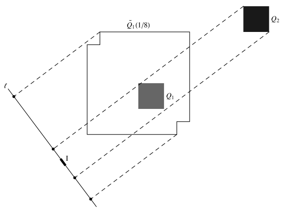
Figure 3. In this figure $Q_{1},Q_{2}\in\mathcal{C}_{I}$. The number $\varepsilon$ (i.e. the length of $I$ relative to the side length of $Q_{1}$ and $Q_{2}$) is chosen so that the projection of $Q_{2}$ onto $\ell$ is contained in the projection of $\widetilde{Q}_{1}(\frac{1}{8})$ whenever $Q_{1}$ is not a corner. When $Q_{1}$ induces a block, the visible part of $E$ from the interval $I$ cannot intersect $Q_{2}$.

The geometric significance of blocks is depicted in Figure 3: Let $Q_{1}$, $Q_{2}\in\mathcal{Q}_{n,j}$ be squares such that $Q_{1}$ is closer to $\ell$ than $Q_{2}$ and $\widetilde{Q}_{1}\neq\widetilde{Q}_{2}$. Suppose that $Q_{1}$ induces a block. Then by the choice of $\varepsilon$ we have

$$\Pi_{\ell}(Q_{2})\subset\Pi_{\ell}(\widetilde{Q}_{1}(\frac{1}{8}))\subset\Pi_{\ell}(\widetilde{Q}_{1}\cap E),$$

giving $Q_{2}\cap V_{\ell}(E)=\emptyset$. In particular, if $Q_{B}\in\mathcal{Q}_{n,j}$ is the first square in $\mathcal{Q}_{n,j}$ that induces a block, then we can cover the visible part of $E$ from $I_{n,j}$ by all chosen squares in $Q_{n,j}$ up to $Q_{B}$, plus the squares $Q$ such that $\widetilde{Q}=\widetilde{Q}_{B}$. Thus, estimates on the position of the first square in $\mathcal{Q}_{n,j}$ that induces a block will yield estimates on the size of $V_{\ell}(E)$.

Letting $\zeta$ and $\eta$ be as in Lemma 2.4, define $\gamma=1-(\zeta+\eta)$ and $\gamma^{\prime}=e^{-\eta^{2}/2}$. Denote by $Y_{n,j}$ the number of chosen squares in $\mathcal{Q}_{n,j}$ which are needed to cover the stripe of $V_{\ell}(E)$ above $I_{n,j}$, and assume that $Y_{n,j}=i+4$. Now there are two possibilities: the number of corners among the first $i$ chosen squares in $\mathcal{Q}_{n,j}$ is either at least $(\zeta+\eta)i$ or less than $(\zeta+\eta)i$.

By Lemma 2.4, the first event has probability at most $\gamma^{\prime i}$ of occurring. In the latter case the number of squares that induce a window among the first $i$ squares is at least $\gamma i$. Observe also that for given $Q\in\mathcal{Q}_{n,j}$ there are at most four $Q^{\prime}\in\mathcal{Q}_{n,j}$ (including $Q$) such that $\widetilde{Q}^{\prime}=\widetilde{Q}$. Hence the probability of the second event is at most $(1-q)^{\frac{\gamma i}{4}}$. We deduce that

$$\mathbf{P}(Y_{n,j}=i+4)\leq(1-q)^{\frac{\gamma i}{4}}+\gamma^{\prime i}\leq 2\tilde{\gamma}^{i}$$

where $\tilde{\gamma}=\max\{(1-q)^{\frac{\gamma}{4}},\gamma^{\prime}\}<1$. This in turn implies that $\mathbf{E}(Y_{n,j})=O(1)$. Writing $S_{n}=\sum_{j=1}^{N(n)}Y_{n,j}$, we therefore have

(3.1) $$\mathbf{E}(S_{n})=O(\varepsilon^{-1}2^{n}).$$

By definition, we can cover $V_{\ell}(E)$ by $S_{n}$ squares of side length $2^{-n}$, whence

$$\mathcal{H}^{1}(V_{\ell}(E))\leq\liminf_{n\rightarrow\infty}\sqrt{2}\cdot 2^{-n}S_{n}.$$

By Fatou’s lemma, Lemma 3.1 below and inequality (3.1), we have that almost surely

$$\mathbf{E}(\mathcal{H}^{1}(V_{\ell}(E)))\leq\liminf_{n\rightarrow\infty}\sqrt{2}\cdot 2^{-n}\mathbf{E}(S_{n})=O(\varepsilon^{-1})<\infty.$$

This shows that $\mathcal{H}^{1}(V_{\ell}(E))<\infty$ almost surely, as desired. ∎

Proof of Corollary 1.6.

The claim follows from Theorem 1.5 combined with Fubini’s theorem. For the purpose of applying Fubini’s theorem we need to prove that the set $\{(E,\ell):0<\mathcal{H}^{1}(V_{\ell}(E))<\infty\}$ is measurable. This is an immediate consequence of Lemma 3.1 in which we prove that it contains a Borel set with full measure. ∎

Let $S_{n}=S_{n}(E,\ell)$ be as in the proof of Theorem 1.5, that is, $S_{n}(E,\ell)$ is the number of the dyadic squares of side length $2^{-n}$ that cover $V_{\ell}(E)$. In the proof of Theorem 1.5 we estimate $S_{n}(E,\ell)$ from above by a function which is defined by counting blocks, windows and corners. Call this function $\widetilde{S}_{n}(E,\ell)$. In the space of constructions we use the natural topology induced by the open cylinder sets $[F]=\{E:E_{m}=\cup_{Q\in F}Q\}$ where $F\subset\mathcal{Q}_{m}$ and $E_{m}$ is the union of all chosen squares of side length $2^{-m}$ in the construction of $E$, that is, $E=\cap_{m=1}^{\infty}E_{m}$.

Lemma 3.1.

The function $(E,\ell)\mapsto\widetilde{S}_{n}(E,\ell)$ is a Borel function for all positive integers $n$.

Proof.

Since the corners are independent of $E$ and $\ell$ we may consider only blocks and windows. Let $N$ be a positive integer. The set $\{(E,\ell):\widetilde{S}_{n}(E,\ell)\leq N\}$ is a finite union of finite intersections of sets of the form $\{(E,\ell):Q\text{ is a block}\}$ and $\{(E,\ell):Q\text{ is a window}\}$ where $Q\in\mathcal{Q}_{n-2}$. Since the latter set is the complement of the former one it suffices to verify that the former one is a Borel set.

From the definition of a block we get

$$\{(E,\ell):Q\text{ is a block}\} = \{(E,\ell):\Pi_{\ell}(Q\cap E)\supset\Pi_{\ell}(Q(\frac{1}{8}))\}$$

$$= \bigcap_{m=1}^{\infty}\{(E,\ell):\Pi_{\ell}(Q\cap E_{m})\supset\Pi_{\ell}(Q(\frac{1}{8}))\}$$

where the last equality follows from the fact that if $y\in\Pi_{\ell}(Q(\frac{1}{8}))$ and $\Pi_{\ell}(Q(\frac{1}{8}))\subset\Pi_{\ell}(Q\cap E_{m})$ for all $m$ then the sets $\Pi_{\ell}^{-1}(y)\cap Q\cap E_{m}$ form a decreasing sequence of non-empty compact sets, and therefore, there exists $x\in\Pi_{\ell}^{-1}(y)\cap E\cap Q$ giving $y\in\Pi_{\ell}(Q\cap E)$.

Given $m$, the set $\mathcal{Q}_{m}$ has a finite number of subsets, say $F_{1},\dots,F_{M}$. Now

$$\{(E,\ell):\Pi_{\ell}(Q\cap E_{m})\supset\Pi_{\ell}(Q(\frac{1}{8}))\}=\bigcup_{i=1}^{M}([F_{i}]\times\{\ell:\Pi_{\ell}(Q\cap\bigcup_{Q^{\prime}\in F_{i}}Q^{\prime})\supset\Pi_{\ell}(Q(\frac{1}{8}))\})$$

is a Borel set since for fixed $i$ the set $\{\ell:\Pi_{\ell}(Q\cap\bigcup_{Q^{\prime}\in F_{i}}Q^{\prime})\supset\Pi_{\ell}(Q(\frac{1}{8}))\}$ consists of finitely many closed intervals. This finishes the proof. ∎

In the last part of this section we prove Theorem 1.3.

Proof of Theorem 1.3.

By Theorem 2.2 (and the results of [FG]) $\operatorname{dim_{H}}V_{\ell}(E)\geq 1$ for all $\ell$ almost surely. Since $\operatorname{dim_{H}}A\leq\operatorname{\underline{dim}_{B}}A\leq\operatorname{\overline{dim}_{B}}A$ for any bounded set $A$, it is enough to show that, given a sequence $a_{n}$ with $\frac{a_{n}}{n}\rightarrow\infty$, almost surely the following holds: if $\ell$ is a line not meeting $Q_{0}$, then

$$N_{n}(V_{\ell}(E))\leq a_{n}2^{n}\quad\textrm{for all large enough }n.$$

Indeed, by Lemma 2.1 it is enough to consider lines which do not meet the unit square, and if the above holds then clearly $\operatorname{\overline{dim}_{B}}V_{\ell}(E)\leq 1$ (taking for example $a_{n}=n^{2}$).

Let $D$ be a closed interval of directions which does not contain the vertical or horizontal ones. Recall that the direction of a line $\ell$ is parametrised by the angle between $\ell^{\perp}$ and the $x$-axis and is denoted by $\theta(\ell)$. It is enough to prove the claim for all lines with directions in $D$ simultaneously, since we can cover all directions by a countable union of such intervals plus the horizontal and vertical directions. Observe that $V_{\ell}(E)=V_{\ell^{\prime}}(E)$ if $\ell^{\prime}$ is parallel to $\ell$ and they both are on the same side of the unit square. By symmetry, $V_{\ell}(E)$ and $V_{\ell^{\prime}}(E)$ still have the same distribution if $\ell^{\prime}$ and $\ell$ are parallel but on different sides of the unit square.

Choose $\varepsilon>0$ such that $\varepsilon<\frac{1}{2}\sin\theta\cos\theta$ for all $\theta\in D$. Consider $n\in\mathbb{N}$ and a line $\ell$ with $\theta(\ell)\in D$. Let $I$ be a line segment of length $\varepsilon 2^{-n}$ in $\Pi_{\ell}(Q_{0})$. We say that a square $Q$ is above $I$ if its centre projects inside $I$ under $\Pi_{\ell}$. Such an interval $I$ is good if either there are fewer than $a_{n}$ chosen squares above $I$, or if there is a chosen square among the first $a_{n}$ chosen squares above $I$ which is not a corner and which induces a block for all $\theta\in D$. Intervals which are not good will be called bad.

Suppose there are at least $a_{n}$ chosen squares above $I$. Letting $\zeta,\eta$ be as in Lemma 2.4 we may, as in the proof of Theorem 1.5, consider the cases in which the number of corners among the first $a_{n}$ chosen squares is at least $(\zeta+\eta)a_{n}$ or less than $(\zeta+\eta)a_{n}$. Arguing exactly like in the proof of Theorem 1.5, but using the full strength of Theorem 2.2 which holds simultaneously for all directions in $D$, we obtain that, for any given interval $I$,

$$\mathbf{P}(I\textrm{ is bad})<e^{-\Omega(a_{n})}.$$

Let $0<\varepsilon^{\prime}<\varepsilon$. Divide $\Pi_{\ell}(Q_{0})$ into line segments of length $\varepsilon^{\prime}2^{-n}$ as in the proof of Theorem 1.5. Let $I_{\ell}^{\prime}$ be such a line segment and let $I\supset I_{\ell}^{\prime}$ be a line segment of length $\varepsilon 2^{-n}$ having the same centre as $I_{\ell}^{\prime}$. Denote by $S_{I}$ the stripe generated by $I$, that is, $S_{I}=I\times\ell^{\perp}$ where $\ell$ is the line containing $I$. Choose $\delta>0$ so small that $S_{I_{\ell_{1}}^{\prime}}\cap Q_{0}\subset S_{I}\cap Q_{0}$ for all $\ell_{1}$ such that

(3.2) $$|\theta(\ell_{1})-\theta(\ell)|<\delta 2^{-n},$$

where $I_{\ell_{1}}^{\prime}$ is the line segment of length $\varepsilon^{\prime}2^{-n}$ in $\Pi_{\ell_{1}}(Q_{0})$ which is closest to $I_{\ell}^{\prime}$. Observe that if $I$ is good then the visible part from $I_{\ell_{1}}^{\prime}$ is covered by the first $a_{n}$ chosen squares above $I$ for all $\ell_{1}$ satisfying (3.2) (or by all such chosen squares if there are fewer than $a_{n}$ of them).

Since for each $\ell$ we need to consider less than $2\varepsilon^{\prime-1}2^{n}$ intervals, the probability that there is at least one interval $I^{\prime}$ such that we cannot cover the visible part above $I^{\prime}$ by at most $a_{n}$ squares of side length $2^{n}$ is less than $2\varepsilon^{\prime-1}2^{n}e^{-\Omega(a_{n})}$. By the above observation, if we have this property for a set of lines $\{\ell_{i}\}$ such that the set of directions $\{\theta(\ell_{i})\}$ is $(\delta 2^{-n})$-dense, then it is true for all directions in $D$. Therefore, the probability that there is some interval $I^{\prime}\subset\Pi_{\ell^{\prime}}(Q_{0})$ for some $\ell^{\prime}$ with $\theta(\ell^{\prime})\in D$ such that we need more than $a_{n}$ squares to cover the visible part from $I^{\prime}$, is bounded above by

$$P_{n}:=4(\delta\varepsilon^{\prime})^{-1}2^{2n}e^{-\Omega(a_{n})}.$$

By our assumption that $\frac{a_{n}}{n}\rightarrow\infty$, the series $\sum_{n}P_{n}$ converges. Hence the Borel-Cantelli lemma implies that almost surely for each $\ell$ with $\theta(\ell)\in D$, the visible part $V_{\ell}(E)$ satisfies

$$N_{n}(V_{\ell}(E))\leq 2\varepsilon^{\prime-1}2^{n}a_{n}\quad\textrm{for all large enough }n.$$

Replacing $a_{n}$ by $a^{\prime}_{n}=a_{n}\varepsilon^{\prime}/2$ we obtain the desired statement. ∎

4. Visible parts from points

In this section we consider visible parts from points. The same general ideas apply, except that we need an analogue of Theorem 2.2 for radial projections. This is given by the following proposition. For $x\in\mathbb{R}^{2}\setminus Q_{0}$, we denote by $\Pi_{x}$ the radial projection onto a circle $S(x)$ centred at $x$ and not intersecting $Q_{0}$.

Proposition 4.1.

Fix $x^{0}\in\mathbb{R}^{2}\setminus Q_{0}$ and let $r_{0}=\frac{1}{10}\min\{1,\operatorname{dist}(x^{0},Q_{0})\}$. Then for any $0<\varepsilon<\frac{1}{2}$ there exists $q_{\varepsilon}>0$ such that

$$\mathbf{P}\bigl{(}\Pi_{x}(E)\supset\Pi_{x}(\underline{Q}_{0}(\varepsilon))\text{ for all }x\in B(x^{0},r_{0})\bigr{)}=q_{\varepsilon}.$$

Here $\underline{Q}_{0}(\varepsilon)$ is the set obtained by removing half-open squares of side length $\varepsilon$ from each corner of the unit square.

The proof of this proposition will be given at the end of this section. We now state the counterparts of Theorems 1.3 and 1.5 for visible parts from points.

Theorem 4.2.

Let $p>\frac{1}{2}$. Conditioned on non-extinction, almost surely

$$\operatorname{dim_{H}}V_{x}(E)=\operatorname{dim_{B}}V_{x}(E)=1$$

for all $x\in\mathbb{R}^{2}\setminus E$. Moreover, if $a_{n}$ is any sequence such that $\frac{a_{n}}{n^{2}}\rightarrow\infty$ as $n\rightarrow\infty$, then almost surely

$$N_{n}(V_{x}(E))\leq a_{n}2^{n}\quad\textrm{for all sufficiently large }n$$

for all $x\in\mathbb{R}^{2}\setminus E$.

Proof.

The counterpart of Lemma 2.1 is valid also in this case, so we may assume that $x\notin Q_{0}$. The proof is similar to the proof of Theorem 1.3 for those $x=(x_{1},x_{2})$ which satisfy $x_{1}\notin[0,1]$ and $x_{2}\notin[0,1]$. In this case the direction of all the rays from $x$ to $Q_{0}$ is at a positive distance from the horizontal/vertical ones. Then for a fixed small enough $\varepsilon>0$ we can divide $\Pi_{x}(Q_{0})$ into arcs of angular length $(|x|+1)^{-1}\varepsilon 2^{-n}$, and then argue like in Theorem 1.3, using Proposition 4.1 instead of Theorem 2.2.

The remaining points induce horizontal or vertical rays. Let $x$ be such a point. To deal with the singularity, we cover the arc $D=\pi_{x}(Q_{0})$ by subarcs $D_{j}$ of length $c2^{-j}$, so that the distance from $D_{j}$ to the vertical/horizontal line is comparable to $\varepsilon_{j}=2^{-j}$.

Now fix a scale $2^{-n}$. The visible part from $x$ along rays in $D_{j}$ with $j>n$ can be covered using all squares in $\mathcal{Q}_{n}$ intersecting such rays; there are $O(2^{n})$ such squares. For each fixed $j\leq n$, we can argue exactly as in the proof of Theorem 1.3 (using Proposition 4.1 instead of Theorem 2.2) to find that the expected number of squares of side length $2^{-n}$ needed to cover the part of $V_{x}(E)$ corresponding to $D_{j}$ is $O(2^{-j}\varepsilon_{j}^{-1}2^{n})=O(2^{n})$. Moreover, writing $b_{n}=\frac{a_{n}}{n}$, the probability that one needs more than $b_{n}2^{n}$ squares is at most $e^{-\Omega(b_{n})}$. Therefore with probability $1-ne^{-\Omega(b_{n})}$ one can cover $V_{x}(E)$ by $nb_{n}2^{n}=a_{n}2^{n}$ squares in $\mathcal{Q}_{n}$.

This argument is for a fixed point $x$, but similarly as in the proof of Theorem 1.3, a bound that works for $x$ works also in a neighbourhood of $x$ (at the cost of losing a constant), and we can cover any bounded part of $\mathbb{R}^{2}\setminus Q_{0}$ by exponentially many such neighbourhoods. The proof then finishes in the same way as the proof of Theorem 1.3. ∎

Theorem 4.3.

Let $p>\frac{1}{2}$. Write

$$\mathcal{D}=\{x=(x_{1},x_{2}):x_{1}\notin[0,1]\textrm{ and }x_{2}\notin[0,1]\}.$$

If $x\in\mathcal{D}$, then $V_{x}(E)$ has finite $\mathcal{H}^{1}$-measure almost surely. For any $x\notin E$, the visible part $V_{x}(E)$ has $\sigma$-finite $\mathcal{H}^{1}$-measure almost surely. Furthermore, conditioned on non-extinction, almost surely

$$0<\mathcal{H}^{1}(V_{x}(E))<\infty$$

for $\mathcal{L}^{2}$-almost all $x\in\mathcal{D}$, and $V_{x}(E)$ has positive and $\sigma$-finite $\mathcal{H}^{1}$-measure for $\mathcal{L}^{2}$-almost all $x\in\mathbb{R}^{2}\setminus E$.

Proof.

If $x\in\mathcal{D}$, then the proof is similar to the proof of Theorem 1.5, with the main modifications being the same ones as in Theorem 4.2.

Now assume that $x_{1}\in[0,1]$ or $x_{2}\in[0,1]$. The value of $\varepsilon$ required becomes $0$ at the horizontal or vertical lines. Hence we consider countably many subarcs covering all directions but horizontal/vertical. As before, the Hausdorff measure of the visible part from each subarc is finite almost surely, so we obtain that $V_{x}(E)$ has $\sigma$-finite measure almost surely, as desired.

The latter assertion follows easily by Fubini’s theorem. ∎

We finish the section with the proof of Proposition 4.1.

Proof of Proposition 4.1.

Let us begin with two remarks. First, it is enough to prove this proposition for some fixed value of $\varepsilon=\varepsilon_{0}$. Indeed, it will immediately imply the assertion for any $\varepsilon>\varepsilon_{0}$. On the other hand, with positive probability all the four first level subsquares belong to $\mathcal{C}_{1}$. Therefore if we know the assertion is satisfied for $\varepsilon_{0}$ for each of them with positive probability, we obtain the assertion for $\frac{\varepsilon_{0}}{2}$. (To see this, it is useful to note that for any $\varepsilon<\frac{1}{2}$, $\underline{Q}_{0}(\varepsilon)$ contains a “plus sign” formed by lines parallel to the sides bisecting the square in two equal parts. Moreover, the union of the projections of the plus signs in each square in $\mathcal{Q}_{1}$ contains the projection of the plus sign in $Q_{0}$.)

The second remark is that we can freely assume that $x^{0}$ is arbitrarily far away from $Q_{0}$. Indeed, again with positive probability all the four first level subsquares belong to $\mathcal{C}_{1}$ and the (relative) distance from $x^{0}$ to each of them is already at least two times greater than the (relative) distance from $x^{0}$ to $Q_{0}$. Repeating this, we only need to know the assertion for $x^{0}$ at very large distance from $Q_{0}$ to prove the assertion for all $x^{0}\in\mathbb{R}^{2}\setminus Q_{0}$.

There will be two cases: $x^{0}$ is in a direction approximately horizontal/vertical from $Q_{0}$, or $x^{0}$ lies in a “diagonal” direction. For notational simplicity we translate the picture so that $Q_{0}$ is centred at the origin. By symmetry, it is enough to consider the cases stated in Lemmas 4.4 and 4.5 below, which completes the proof. ∎

Lemma 4.4.

The assertion of Proposition 4.1 is satisfied for $\varepsilon=\frac{1}{4}$ and $x^{0}=(x_{1},x_{2})$ such that $x_{2}<0$, $x_{1}<-N_{1}$ and $\frac{x_{1}}{x_{2}}>N_{1}$ for $N_{1}$ large enough.

Proof.

Let us introduce some notation. We will call a line $\ell$ passing through a square $Q$ if it intersects two parallel sides of $Q$. Note that, provided $N_{1}$ is sufficiently large, any line containing $x\in B(x^{0},r_{0})$ and intersecting $Q_{0}(\frac{1}{4})$ is passing through one of the sixteen second level subsquares of $Q_{0}$ (hitting their vertical sides). As each of those subsquares has positive probability of belonging to $\mathcal{C}_{2}$, it is enough to prove that with positive probability all the lines containing $y\in B(y^{0},r_{0})$ and passing through $Q_{0}$ intersect $E$, where $y^{0}=(y_{1},y_{2})$ satisfies $y_{2}<0$, $y_{1}<-4N_{1}$ and $\frac{y_{1}}{y_{2}}>\frac{N_{1}}{2}$.

Given $k\in\mathbb{N}$ and $z\in\Pi_{y}(Q_{0})$, let $V_{k}(y,z)$ be the number of squares $Q\in\mathcal{C}_{k}$ passed by the line $\ell(y,z)$ going through $y$ and $z$. We denote by $Z_{y}$ the subarc of $\Pi_{y}(Q_{0})$ determined by the lines $\ell(y,z)$ passing through $Q_{0}$.

Let $n$ be so large that

(4.1) $$(2^{n}-1)p^{n}>2$$

and let $N_{1}=2^{n+1}$. This is the point where we use that $p>\frac{1}{2}$. As is easy to check, every line containing $y$ and passing through $Q_{0}$ intersects at most $2^{n}+1$ of the $n^{\text{th}}$ level subsquares of $Q_{0}$, passing through at least $2^{n}-1$ of them. Hence, by (4.1), for each of those lines the expected number of squares in $\mathcal{C}_{n}$ passed by the line is greater than 2.

We want to apply an appropriate large deviation theorem to show that with positive probability, for each $y$ and $z$ the function $V_{k}(y,z)$ will actually increase exponentially fast with $k$. This will in particular imply that $\ell(y,z)$ has non-empty intersection with $\bigcup_{\mathcal{C}_{k}}Q$ for all $k$, thus with $E$ as well, which is precisely the statement we need.

We parametrise the space of lines $L=\{\ell(y,z):y\in B(y^{0},r_{0}),z\in Z_{y}\}$ by their intersection point with the vertical line $x_{1}=-5N_{1}$ and by the angle they make with the $x$-axis. We call this parameter set $P$. (The particular parametrisation chosen is not important.)

Denote by $\{w_{i}^{(k)}\}$ the set of corner points of all subsquares of $Q_{0}$ of level $k$. For each $i$ the condition $w_{i}^{(k)}\in\ell(y,z)$ defines a smooth curve $\gamma_{i}$ on $P$. These curves divide $P$ into components denoted by $\{C_{j}^{(k)}\}$. Each $C_{j}^{(k)}$ is such that for any two lines $\ell_{1},\ell_{2}\in C_{j}^{(k)}$ the set of subsquares of $Q_{0}$ of level $k$ passed by $\ell_{1}$ and by $\ell_{2}$ is the same (and the boundary lines of each $C_{j}^{(k)}$ pass through the same subsquares the other lines in $C_{j}^{(k)}$ pass through, plus possibly some additional ones). Hence, $V_{k}(y,z)$ is constant on each $C_{j}^{(k)}$ (and can only increase at the boundary points).

We claim that the number of these components is at most $2^{4k}$. Note that the components are faces of the planar graph whose vertices are the intersection points of the curves $\gamma_{i}$ and edges are the pieces of $\gamma_{i}$ between vertices. By Euler’s theorem, the number of faces is less than twice the number of vertices. Since there is at most one line going through $w_{i}^{(k)}$ and $w_{j}^{(k)}$ for $i\neq j$, $\gamma_{i}$ and $\gamma_{j}$ intersect at most once. Thus the number of vertices is at most $\frac{N^{2}}{2}$, where $N=(2^{k}+1)^{2}$ is the number of corner points. This yields our claim.

For each $k\geq 1$, let $\{\ell(y_{j}^{(kn)},z_{j}^{(kn)})\}$ be a collection of representatives of the components $\{C_{j}^{(kn)}\}$. Let $A_{k,j}$ be the event

$$V_{kn}(y_{j}^{(kn)},z_{j}^{(kn)})\geq 2^{k}.$$

Further, let $A_{k}=\bigcap_{j}A_{k,j}$. Because of the way the components $C_{j}^{(kn)}$ were defined, it will be enough to show that $\mathbf{P}(\cap_{k=1}^{\infty}A_{k})=\Omega(1)$.

There is a positive probability that $V_{n}(y,z)\geq 2$ for all $\ell(y,z)\in P$. Indeed, it is enough that all squares of generation $n$ are chosen. Thus, $p_{0}:=\mathbf{P}(A_{1})>0$.

Now suppose that $A_{k}$ holds, and consider a line

$$\ell_{j}=\ell(y_{j}^{((k+1)n)},z_{j}^{((k+1)n)}).$$

By assumption, $\ell_{j}$ passes through at least $2^{k}$ squares in $\mathcal{C}_{kn}$. By (4.1), if $Q$ is one of these squares, the expected number of squares in $\mathcal{C}_{(k+1)n}$ that $\ell_{j}$ hits inside $Q$ is strictly greater than $2$. Thus, conditioned on $\mathcal{C}_{kn}$, $V(y_{j}^{((k+1)n)},z_{j}^{((k+1)n)})$ is the sum of at least $2^{k}$ i.i.d. bounded random variables with expectation $E>2$. Note that the distribution of these random variables is independent of $k$. By standard large deviation results (for example one could use the Azuma-Hoeffding inequality [ASE, Theorem 7.2.1] as in the proof of Lemma 2.4), we see that

$$\mathbf{P}(V(y_{j}^{((k+1)n)},z_{j}^{((k+1)n)})\geq 2^{k+1})\geq 1-\gamma^{2^{k}},$$

for some $\gamma<1$ which does not depend on $k$ or $j$. In other words, $\mathbf{P}(A_{k+1,j})\geq 1-\gamma^{2^{k}}$.

The events $A_{k,j}$ are clearly increasing, whence we can apply the FKG-inequality [G, Theorem 2.4] to obtain

$$\mathbf{P}(A_{k})\geq\prod_{j}\mathbf{P}(A_{k,j})\geq(1-\gamma^{2^{k}})^{2^{4(k+1)n}}.$$

Therefore

$$\mathbf{P}\left(\bigcap_{k=1}^{\infty}A_{k}\right) =\mathbf{P}(A_{1})\prod_{k=1}^{\infty}\mathbf{P}(A_{k+1}|A_{k})$$

$$\geq p_{0}\prod_{k=1}^{\infty}\left(1-\gamma^{2^{k}}\right)^{2^{4(k+1)n}}.$$

Since $\gamma^{2^{k}}$ goes to $0$ superexponentially fast while $2^{4(k+1)n}$ grows only exponentially fast, the infinite product converges. This completes the proof. ∎

The second case was essentially done in [RS] and the proof is very similar to the proof of Lemma 4.4, but for completeness we will remind here the basic steps of the proof. At the same time, since the proof is very similar, we give a sketch of the proof of Theorem 2.2.

Lemma 4.5.

There exists $N_{2}>0$ such that if $x^{0}=(x_{1},x_{2})$ satisfies $x_{1}<0$, $x_{2}<0$, $1\leq x_{1}/x_{2}<N_{1}$ and $x_{1}+x_{2}<-N_{2}$ then the assertion of Proposition 4.1 is satisfied for $x^{0}$ with $\varepsilon=\frac{1}{4}$.

Proof.

We begin with some notation. Given $Q$, a subsquare of $Q_{0}$, let $I_{1}(Q)$ and $I_{2}(Q)$ be the squares with the same centre as $Q$ and having side length $\lambda_{1}$ and $\lambda_{2}$ times the side length of $Q$, respectively, where

$$0<\lambda_{2}<\lambda_{1}<1.$$

Note that $I_{2}(Q)$ is contained in the interior of $I_{1}(Q)$.

Given a line $\ell$, which is neither horizontal nor vertical, we define

$$V_{k}^{(1)}(z)=\sharp\{Q\in\mathcal{C}_{k}:z\in\Pi_{\ell}(I_{1}(Q))\}$$

and

$$V_{k}^{(2)}(z)=\sharp\{Q\in\mathcal{C}_{k}:z\in\Pi_{\ell}(I_{2}(Q))\},$$

where the number of elements in a set $A$ is denoted by $\sharp A$. Let $\widetilde{V}_{k}^{(1,2)}$ be the version of the above, where $\Pi_{\ell}$ is replaced by $\Pi_{x}$.

An observation in [RS] is that if $p>\frac{1}{2}$ then for each $\ell$ one can choose $\lambda_{1}$ and $\lambda_{2}$ such that for some $n$ and for all $z\in\Pi_{\ell}(Q_{0})$ we have

$$\mathbf{E}(V_{k+n}^{(2)}(z))>2V_{k}^{(1)}(z).$$

A similar statement can be obtained for $\widetilde{V}_{k}^{(i)}$, provided $x$ is sufficiently far away from $Q_{0}$ (the necessary distance depends on the direction in which $x$ lies, and blows up for horizontal and vertical directions. Note that the near-horizontal and near-vertical cases are dealt with in Lemma 4.4.)

Similarly to the proof of Lemma 4.4, we can then check that if, for some finite family $\{z_{i}^{(k+1)n}\}$ of cardinality $K$, one has that

(4.2) $$V_{kn}^{(1)}(z_{i}^{((k+1)n)})>M,$$

then with probability $(1-(1-\Omega(1))^{M})^{K}$,

(4.3) $$V_{(k+1)n}^{(2)}(z_{i}^{(k+1)n})>2M$$

(and similarly for $\widetilde{V}_{kn}^{(1)}$, $\widetilde{V}_{(k+1)n}^{(2)}$). With positive probability (e.g. corresponding to the probability that all squares of level $n$ are chosen), the equation (4.2) is satisfied for $k=1$ for all $z\in\Pi_{\ell}(Q_{0}(\frac{1}{4}))$ (resp. $z\in\Pi_{x}(\underline{Q}_{0}(\frac{1}{4}))$for $\widetilde{V}^{(1)}_{kn}$).

As $I_{2}(Q)\subset I_{1}(Q)$, whenever $z$ belongs to the projection of $I_{2}(Q)$, all $y$ close to $z$ belong to the projection of $I_{1}(Q)$. Hence, if the implication (4.2) $\Rightarrow$ (4.3) holds for a finite family $\{z_{i}^{(k+1)n}\}$ (of size $K$ increasing only exponentially fast with $k$), then

(4.4) $$V_{(k+1)n}^{(1)}(z)>2M$$

for all $z\in\Pi_{\ell}(Q_{0}(\frac{1}{4}))$ (resp. $z\in\Pi_{x}(\underline{Q}_{0}(\frac{1}{4}))$ for $\widetilde{V}^{(1)}_{(k+1)n}$). Note that the family $\{z_{i}^{(k+1)n}\}$ takes the place of the components in the proof Lemma 4.4.

An inductive argument completely analogous to the proof of Lemma 4.4 then allows us to conclude that

$$\mathbf{P}\left(V_{kn}^{(1)}(z)\geq 2^{k}\textrm{ for all }z\in\Pi_{\ell}(Q_{0}(\frac{1}{4}))\right)>0,$$

and likewise

$$\mathbf{P}\left(\widetilde{V}_{kn}^{(1)}(z)\geq 2^{k}\textrm{ for all }z\in\Pi_{\ell}(\underline{Q}_{0}(\frac{1}{4}))\right)>0.$$

This finishes the proof. ∎

References

- [ASE] N. Alon, J. H. Spencer and P. Erdös, The Probabilistic Method, John Wiley & Sons, Inc, New York, 1992.
- [C] L. Chayes, Aspects of the fractal percolation process, Bandt, C., Graf, S., Zähle, M. (eds.), Fractal Geometry and Stochastics, Birkhäuser, Basel, 1995.
- [CCD] J. T. Chayes, L. Chayes and R. Durrett, Connectivity Properties of Mandelbrot’s Percolation Process, Probab. Th. Rel. Fields 77, 307–324 (1988).
- [Cs] M. Csörnyei, On the visibility of invisible sets, Ann. Acad. Sci. Fenn. Math. 25, 417–421, 2000.
- [FG] K. J. Falconer and G. R. Grimmett, On the Geometry of Random Cantor Sets and Fractal Percolation, J. Theor. Prob. 5, 465–485 (1992).
- [FGc] K. J. Falconer and G. R. Grimmett, On the Geometry of Random Cantor Sets and Fractal Percolation, J. Theor. Prob. 7, 209–210 (1994).
- [G] G. Grimmett, Percolation, second edition, Springer-Verlag, Berlin, 1999.
- [JJMO] E. Järvenpää, M. Järvenpää, P. MacManus and T. C. O’Neil, Visible parts and dimensions, Nonlinearity 16 (2003), 803-818.
- [J] M. Järvenpää, Visibility and fractal percolation, International Conference on Complex Analysis and Related Topics, Alba Iulia, 2008, to appear.
- [M1] P. Mattila, Geometry of Sets and Measures in Euclidean Spaces: Fractals and rectifiability, Cambridge University Press, Cambridge, 1995.
- [M2] P. Mattila, Hausdorff dimension, projections, and the Fourier transform, Publ. Math. 48 (2004), 3-48.
- [O] T. C. O’Neil, The Hausdorff dimension of visible sets of planar continua, Trans. Amer. Math. Soc. 359 (2007), 5141-5170.
- [PS] Y. Peres and W. Schlag, Smoothness of projections, Bernoulli convolutions, and the dimension of exceptions, Duke Math. J 102 (2000), 193–251.
- [RS] M. Rams and K. Simon, Projection properties of Mandelbrot percolations, in preparation.