Convergence and performances of the peeling wavelet denoising algorithm

Abstract.

This note is devoted to an analysis of the so-called peeling algorithm in wavelet denoising. Assuming that the wavelet coefficients of the signal can be modeled by generalized Gaussian random variables, we compute a critical thresholding constant for the algorithm, which depends on the shape parameter of the generalized Gaussian distribution. We also quantify the optimal number of steps which have to be performed, and analyze the convergence of the algorithm. Several versions of the obtained algorithm were implemented and tested against classical wavelet denoising procedures on benchmark and simulated biological signals.

1. Introduction

Among the wide range of applications of wavelet theory which have emerged during the last 20 years, the processing of noisy signals is certainly one of the most important one. Especially attractive to the community has been the thresholding algorithm, and the great amount of efforts in this direction is well represented by the enthusiastic discussion in [7], by the application oriented presentation [1] or by the sharp uniform central limit theorems in [8]. This fundamental algorithm can be summarized in the following way: recall that the wavelet decomposition of a function $z\in L^{2}(\mathbb{R})$ is usually written as:

$$z(t)=\sum_{k=0}^{2^{j_{0}}-1}\alpha_{j_{0}k}\phi_{j_{0}k}(t)+\sum_{j=j_{0}}^{\infty}\sum_{k=0}^{2^{j}-1}\beta_{jk}\psi_{jk}(t),$$ (1)

where the coefficients $\alpha,\beta$ are obtained by projection in $L^{2}(\mathbb{R})$:

$$\alpha_{j_{0}k}=\left\langle\phi_{j_{0}k},z\right\rangle_{L^{2}(\mathbb{R})},\quad\mbox{and}\quad\beta_{jk}=\left\langle\psi_{jk},z\right\rangle_{L^{2}(\mathbb{R})}.$$

The functions $\psi$ and $\phi$ are respectively called mother and father wavelets, and enjoy some suitable scaling and algebraic properties (see e.g. [5, 12] for a complete account on wavelet decompositions). In this context, the thresholding algorithm assumes that, if $z$ can be decomposed into $z=x+n$, where $x$ is the useful signal and $n$ its noisy part, then the wavelet coefficients corresponding to $n$ will typically be very small. A reasonable estimation for the signal $x$ is thus:

$$\hat{x}(t)=\sum_{k=0}^{2^{j_{0}}-1}\alpha_{j_{0}k}\,{\bf 1}_{\{|\alpha_{j_{0}k}|\geq\tau\}}\,\phi_{j_{0}k}(t)+\sum_{j=j_{0}}^{J}\sum_{k=0}^{2^{j}-1}\beta_{jk}\,{\bf 1}_{\{|\beta_{jk}|\geq\tau\}}\,\psi_{jk}(t),$$

where $\tau$ is a suitable threshold (which may also depend on the resolution $j$ and, in practice, is often null for the coefficients $\alpha_{j_{0}}$ of the father wavelet / scale function) and where $J$ corresponds to the maximal resolution one is allowed to consider. It is then proved in the aforementioned references [1, 7] that this kind of estimator satisfies some nice properties concerning the asymptotic behavior of the approximation error, in terms of the total number of wavelet coefficients (which is denoted by $N$ in the sequel).

One of the drawbacks of the thresholding algorithm is that it may also spoil the original signal $x$. The critical issue is the value of the threshold(s) $\tau$: too low it is inefficient, too high it distorts the information from $x$. In order to improve the performances of wavelet-based denoising algorithms by adapting them to the processed signals, the following iterative method, called peeling algorithm, has been introduced and shown to be particularly useful for biomedical applications in [4, 9]. It still relies on an a priori decomposition of the observed signal $z$ into $z=x+n$, where $x$ is the signal itself, and $n$ is a noise. The algorithm intends then to separate $x$ from $n$ iteratively, and the $k\textsuperscript{th}$ step of the procedure produces an estimated signal $x_{k}$, and a noise $n_{k}$, initialized for $k=0$ as $n_{0}=z$. These functions will always be assimilated with the vector of their wavelet coefficients. Then the $(k+1)\textsuperscript{th}$ step is as follows:

1. Compute $\sigma_{k}^{2}=\frac{\|n_{k}\|^{2}}{N}$, where we recall that $N$ denotes the total number of wavelet coefficients involved in the analysis.

2. Set a thresholding level $T_{k+1}$ as $T_{k+1}=h(\sigma_{k})$, where $h$ is usually linear, which means that $T_{k+1}=F\,\sigma_{k}$ for a certain coefficient $F$.

3. Compute $\Delta x_{k+1}$ as:

   $$\Delta x_{k+1}(q)=n_{k}(q)\,{\bf 1}_{\{|n_{k}(q)|\geq T_{k+1}\}},$$

   for all the coefficients $q$ of the wavelet decomposition. The vectors $x_{k+1},n_{k+1}$ are then defined as $x_{k+1}=x_{k}+\Delta x_{k+1}$, and $n_{k+1}=n_{k}-\Delta x_{k+1}$.

4. Loop this procedure until a stop criterion of the form $\|n_{k}\|^{2}-\|n_{k+1}\|^{2}\leq\varepsilon$ is reached, for a certain positive constant $\varepsilon$. Notice that one can choose $\varepsilon=0$.

This iterative procedure tends to retrieve a higher quantity of (approximate) signal $x$ from the noisy input $z$, correcting some of the failures of the original thresholding algorithm in some special situations.

On the basis of these promising experimental results, the peeling algorithm has been further investigated in [14, 15], and it has been first observed in those references that the peeling problem could be handled through a fixed point algorithm. This possibility stems basically from the fact that the sequence $\{T_{k};\,k\geq 0\}$ is decreasing (as $\|n_{k}\|^{2}\geq\|n_{k+1}\|^{2}$), which means that the previous algorithm can be reduced to the following:

1. Set $T_{0}=+\infty$ and $T_{k+1}=f_{N}(T_{k})$, where $f_{N}$ is of the form:

   $$f_{N}(x)=F\ \left[\frac{\sum_{q\leq N}z^{2}(q)\,{\bf 1}_{\{|z(q)|<x\}}}{N}\right]^{1/2}.$$ (2)

   For a suitable constant $F$, this defines a converging decreasing sequence $(T_{k})$, such that $\lim_{k\to\infty}T_{k}=T_{f}>0$.

2. Stop the loop when $T_{k+1}=T_{f}$, and then set

   $$\hat{x}(q)=z(q)\,{\bf 1}_{\{|z(q)|\geq T_{f}\}}.$$ (3)

It is shown in [14] that this algorithm is almost surely convergent, and a further analysis of the coefficient $F$ is performed in [15].

However, in spite of the efforts made in the aforementioned references [14, 15], a probabilistic analysis of the algorithm is still missing. The current article proposes to make a step in this direction, and we proceed now to describe the results we have obtained. First of all, let us say a few words about the model we have chosen for our signal $z$. This signal is of course characterized by the family of its wavelets coefficients, which will be denoted from now on by $\{z(q);\,q\leq N\}$, and it is usual in signal processing to model these coefficients by independent generalized Gaussian variables (see e.g. [13]), all defined on a common complete probability space $(\Omega,\mathcal{F},P)$. To be more specific, we will assume the following:

Hypothesis 1.1.

The wavelet coefficients $\{z(q);\,q\leq N\}$ of our signal $z$ form an i.i.d family of generalized Gaussian variables, whose common density $(p_{\sigma,u}(x))_{x\in\mathbb{R}}$ is given by

$$p_{\sigma,u}(x)=\alpha e^{-|\beta x|^{u}},\quad\mbox{with}\quad\beta=\frac{1}{\sigma}\left(\frac{\Gamma(3/u)}{\Gamma(1/u)}\right)^{1/2},\quad\alpha=\frac{\beta u}{2\Gamma(1/u)},$$ (4)

where $\Gamma$ stands for the usual Gamma function $\Gamma(\xi)=\int_{0}^{\infty}e^{-x}x^{\xi-1}dx$. Notice that the coefficient $\sigma>0$ above is the standard deviation of each random variable $z(q)$, and that $u>0$ represents the shape parameter of the probability law ($u=2$ for the Gaussian, $u=1$ for the Laplace pdf).

It should be stressed at this point that this model does not take into account the possible decomposition of $z$ into a signal plus a noise, since we model directly the wavelet coefficients of $z$. It is however suitable for the main example we have in mind, namely a situation where the family $\{z(q);\,q\leq N\}$ is sparse. Indeed, when $u<2$ in expression  (4), the distribution of the $z(q)$’s becomes heavy tailed, which means that one expects a few large coefficients and many small ones. This is the situation we are mostly interested in, but our analysis below is valid for any coefficient $u>0$ once our basic model is assumed to be realistic. It should also be stressed that in the end, our algorithm is also of thresholding type, as may be seen from equation (3). This means in particular that it is certainly suitable to retrieve signal from a noisy input, on the same basis as the original thresholding algorithm.

With these preliminary considerations in mind, here are the two main results which will be presented in this paper:

(1) We have seen that the sequence of thresholds $\{T_{k};\,k\geq 0\}$ involved in the peeling algorithm converges almost surely. However, it is easily checked that it can converge either to a strictly positive quantity $T_{f}$, either to 0. This latter limit is not suitable for our purposes, since it means that no noise will be extracted from our signal. One of the main questions raised by the peeling algorithm is thus to find an appropriate constant $F$ in (2) such that (i) The algorithm yields a convergence to a non trivial threshold $T_{f}>0$. (ii) $F$ is small enough, so that a sufficient part of the original signal is retrieved.

The previous attempts in this direction were simply (see [9]) to take $F=3\sigma$ with experimental arguments; after the analysis performed in [15], this quantity was reduced to $F=F_{m}$, a quantity which is defined by

$$F_{m}=\sqrt{\frac{3\Gamma(1/u)}{u}(ue)^{1/u}}.$$ (5)

However, the latter bound has been obtained thanks to some rough estimates, and we have thus decided here to go one step further into this direction. Indeed, our first task will be to determine precisely, and on a mathematical ground, a constant $F_{c}=F_{c}(u,\sigma)$ such that: if $F>F_{c}$, the algorithm yields a convergence, with high probability, to a strictly positive constant $T_{f}=T_{f}(\omega)$, whose fluctuations around a typical non-random value $x^{*}$ will be determined. In particular, we will see that our constant $F_{c}$ is always lower than $F_{m}$. Whenever $F<F_{c}$, we also show that $T_{k}$ converges to 0 with high probability (see Proposition 3.5).

(2) In the regime $F>F_{c}$, we determine that the optimal number of steps for the peeling algorithm is of order $\log(N)$, where we recall that $N$ is the total number of wavelet coefficients involved in the analysis. After this optimal number of steps, Theorem 3.3 quantifies also sharply the oscillations of $T_{f}$ with respect to its theoretical value $m_{f}$.

It is important to show that our theoretical results can really be applied to real data. We have thus decided first to compare the performances of our algorithm with other wavelet denoising procedures, on some classical benchmark signals proposed in [6]. It will be seen that our algorithm performs well with respect to other methods, independently of the value of the shape parameter in (4) and of the form of the benchmark signal. Interestingly enough, this assertion is true even if Hypothesis 1.1 is not always satisfied by the benchmark signals under consideration.

A second step in our practical part of the study is the following: since the peeling algorithm has been introduced first in a medical context, we give an illustration of its performances on ECG type signals. More specifically, we shall consider a simulated ECG signal, and observe the denoising effect of our algorithm on a perturbed version of those electrocardiograms. It will be observed again that the algorithm under analysis is a good compromise between denoising and preservation of the original signal.

Let us mention some open problems that have been left for a subsequent publication: first, let us recall that the so-called block thresholding has improved the behavior of the original thresholding algorithm in a certain number of situations (see e.g. [2] for a nice overview). It would be interesting to analyze the effect of this procedure in our peeling context. In relation to this problem, one should also care about some reasonable dependence structure among wavelet coefficients, beyond the independent case treated in this article. Finally, we have assumed in this paper that the parameters of the distribution $p_{\sigma,u}$ were known, which is typically not true in real world applications. One should thus be able to quantify the effect of parameter estimation on the whole denoising process.

Here is how our article is structured: we show how to compute optimal constants for the peeling algorithm at Section 2. Then the probabilistic analysis of the algorithm is leaded at Section 3. Finally, some numerical experiment on simulated and pseudo-real data are performed at Section 4.

2. Critical constants for the peeling algorithm

This section is devoted to the computation of an optimal constant $F$ in equation (2), ensuring a convergence of the threshold $T_{k}$ to a non trivial $T_{f}$, and still allowing to retrieve a maximal amount of approximate signal from our noisy input $z$.

Let us start this procedure by changing slightly the setting of the peeling algorithm. Indeed, it will be essential for our convergence theorems at Section 3, to be able to express the fixed point algorithm in terms of empirical processes. To this purpose, we resort to a simple change of variables by setting:

$$U_{k}=T_{k}^{2},\quad\mbox{and}\quad Y(q)=z(q)^{2}.$$

Note that $U_{0}=+\infty$. It is then readily checked that the fixed point algorithm of Section 1 is equivalent to the following:

1. $U_{k+1}=g_{N}(U_{k})$, where $g_{N}$ is of the form:

   $$g_{N}(x)=\frac{F^{2}}{N}\sum_{q\leq N}Y(q)\,{\bf 1}_{\{Y(q)<x\}}.$$

   For a suitable constant $F$, this defines a converging decreasing sequence $(U_{k})$, such that $\lim_{k\to\infty}U_{k}=U_{f}$.

2. Stop the loop when $U_{k+1}=U_{f}$, and then set

   $$\hat{x}(q)=z(q)\,{\bf 1}_{\{|z(q)|\geq\sqrt{U_{f}}\}}.$$

The fixed point $U_{f}=U_{f}(\omega)$ is then solution of the equation $g_{N}(x)=x$. We wish to find the critical (minimal) $F$ which ensures $U_{f}$ to be strictly positive.

A preliminary step towards this aim is to consider a natural deterministic problem related to the equation $g_{N}(x)=x$. Indeed, for a fixed value of $x\in\mathbb{R}_{+}$, the law of large numbers asserts that the random variable $g_{N}(x)$ converges almost surely to the quantity

$$g_{\sigma,u}(x)=F^{2}\int_{0}^{x}w\hat{p}_{\sigma,u}(w)\,dw,$$

where $\hat{p}_{\sigma,u}$ is the common density of the random variables $Y(q)=z(q)^{2}$, given explicitly under Hypothesis 1.1 by

$$\hat{p}_{\sigma,u}(w)=\frac{p_{\sigma,u}(\sqrt{w})}{\sqrt{w}}{\bf 1}_{\{w>0\}}=\alpha\frac{1}{\sqrt{w}}e^{-(\beta\sqrt{w})^{u}}{\bf 1}_{\{w>0\}}.$$ (6)

This result is only a simple convergence result, and not an almost sure uniform convergence of $g_{N}$ towards $g_{\sigma,u}$. However, as will be shown in the Section 3, the fixed point $U_{f}$ is close in some sense to a fixed point of $g_{\sigma,u}$. Therefore, our study of the fixed points of $g_{N}$ can be reduced to the study of $g_{\sigma,u}$. Our aim is now to give some sharp conditions on the coefficient $F$ ensuring that the equation $g_{\sigma,u}(x)=x$ has at least one solution $x>0$.

According to (6) we obtain, for $x>0$:

$$g_{\sigma,u}(x)=F^{2}\alpha\int_{0}^{x}\sqrt{w}e^{-(\beta\sqrt{w})^{u}}dw,$$

with $\beta=\frac{1}{\sigma}\left(\frac{\Gamma(3/u)}{\Gamma(1/u)}\right)^{1/2}$ and $\alpha=\frac{\beta u}{2\Gamma(1/u)}.$ Furthermore, a simple change of variables argument yields:

$$g_{\sigma,u}(x)=F^{2}\sigma^{2}\Gamma_{{\rm inc}}((\beta\sqrt{x})^{u},3/u)$$ (7)

where $\Gamma_{{\rm inc}}(x,a)=\frac{1}{\Gamma(a)}\int_{0}^{x}e^{-t}t^{a-1}dt$ is the incomplete Gamma function.

Observe that the trivial change of variables $w=\sigma^{2}y$ in the integral above yields the expression:

$$g_{\sigma,u}(x)=\,\sigma^{2}g_{1,u}(x/\sigma^{2})$$ (8)

Hence, solving $g_{\sigma,u}(x)=x$ is equivalent to solve $g_{1,u}(v)=v$, for $v=x/\sigma^{2}$. We shall consider our equation in this reduced form, since $\sigma$ has only a scale role in the fixed point problem of $g_{\sigma,u}$ and can be omitted in the study. In the sequel, we thus solve the problem in its reduced form: $g_{1,u}(x)=x$. Furthermore, for notational sake, we simply denote $g_{1,u}$ by $g$.

The resolution of the equation $g(x)=x$ boils down to the joint study of $g$ and of a function $d$ defined by $d(x)=g(x)-x$. These studies are a matter of elementary considerations, and it is easily deduced that $g$ has the following form, as a function from $\mathbb{R}_{+}$ to $\mathbb{R}_{+}$:

1. $g$ is increasing and $\lim_{x\to\infty}g(x)=F^{2}\triangleq g_{\infty}$.

2. $g$ is convex on $[0,\beta^{-2}u^{-2/u}]$ and concave on $[\beta^{-2}u^{-2/u},+\infty)$, where $\beta=\left(\frac{\Gamma(3/u)}{\Gamma(1/u)}\right)^{1/2}$.

More precisely, it is easy to prove the existence of a critical value $F_{c}$ such that:

1. If $F<F_{c}$, the only fixed point of $g$ is 0.

2. If $F=F_{c}$, $g$ has exactly two fixed points (0 and $x^{*}_{c}>\beta^{-2}u^{-2/u}$).

3. If $F>F_{c}$, $g$ has exactly three fixed points (0, $l_{1}$, and $x^{*}$), such that $0<l_{1}<x^{*}$ and $\beta^{-2}u^{-2/u}<x^{*}$.

These facts are well illustrated by Figure 1 (for $\sigma=1$).

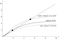
Figure 1. Curves corresponding to $g$, in the critical case ($F=F_{c}$), and in supercritical and subcritical cases ($F=1.15F_{c}$ and $F=0.9F_{c}$), for $\sigma=1$ and $u=2$.

Let us turn now to the computation of the critical coefficient $F_{c}$ and the critical fixed point $x^{*}_{c}$. In fact, once the study of our function $d$ is performed, it is also easy to show that $F\equiv F_{c}$ and $r\equiv x^{*}_{c}$ are solutions of the system:

$$g^{\prime}(r)=1,\quad\mbox{and}\quad g(r)=r,$$

where we recall that the coefficient $F$ enters into the definition of $g$. This system is equivalent, in the generalized Gaussian case, to:

$$\begin{cases}F^{2}\alpha\sqrt{r}e^{-(\beta\sqrt{r})^{u}}-1&=0\\ F^{2}\Gamma_{\rm inc}((\beta\sqrt{r})^{u},3/u)-r&=0,\end{cases}$$

where it should be reminded that $\Gamma$ and $\Gamma_{\rm inc}$ designate respectively Gamma and incomplete Gamma functions. The latter system can be solved with the Mathematica software, and the solutions for different $u$ are illustrated in Figure 2.

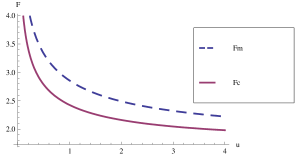
Figure 2. The values of critical $F_{c}$ and $F_{m}$ for $\sigma=1$ and $u\in[0,4]$.

Some typical values of $F_{c}$ in terms of $u$ are also given in Table 1.

$u$	0.1	0.5	1	2	3	4
$F_{c}$	4.0215	2.7830	2.42537	2.16169	2.0472	1.98181

Table 1. Critical constant $F_{c}$ for different shapes $u$.

In particular, it can be observed that $F_{c}$ is smaller than the bound $F_{m}$ proposed by [15], which has been recalled at equation (5).

3. Probabilistic analysis of the algorithm

3.1. Comparison Noisy dynamics/ Deterministic dynamics

The exact dynamics governing the sequence $\{U_{n};\,n\geq 0\}$ is of the form $U_{n+1}=g_{N}(U_{n})$. In order to compare this with the deterministic dynamics, let us recast this relation into:

$$U_{n+1}=g(U_{n})+\varepsilon_{n,N},\quad\mbox{where}\quad\varepsilon_{n,N}=g_{N}(U_{n})-g(U_{n}).$$

Notice that the errors $\varepsilon_{n,N}$ are far from being independent, which means that the relation above does not define a Markov chain. However, a fairly simple expression is available for $U_{n}$:

Proposition 3.1.

For $n\geq 0$, set $g^{\circ n}$ for the $n$^th iteration of $g$. Then, for $n\geq 0$, we have:

$$U_{n}=g^{\circ n}(U_{0})+R_{n},\quad\mbox{with}\quad R_{n}=\sum_{p=0}^{n-1}\varepsilon_{p,N}\prod_{q=2}^{n-p}g^{\prime}(C_{p+q}),$$

where the random variable $C_{j}$ ($j\geq 2$) is a certain real number within the interval $[g^{\circ(j-1)}(U_{0});$ $U_{j-1}]$. In the definition of $R_{n}$, we have also used the conventions $\prod_{q=2}^{1}a_{q}=1$ and $R_{0}=0$.

Proof.

It is easily seen inductively that $R_{0}=0$, $R_{1}=\varepsilon_{0,N}$ and for $n\geq 1$

$$R_{n+1}=g^{\prime}(C_{n+1})R_{n}+\varepsilon_{n,N}.$$

Hence, by a backward induction, we obtain:

$$R_{n}=\sum_{j=1}^{n}\varepsilon_{n-j,N}\prod_{l=0}^{j-2}g^{\prime}(C_{n-l})=\sum_{p=0}^{n-1}\varepsilon_{p,N}\prod_{q=2}^{n-p}g^{\prime}(C_{p+q}),$$

which ends the proof. ∎

A useful property of the errors $\varepsilon_{p,N}$ is that they concentrate exponentially fast (in terms of $N$) around 0. This can be quantified in the following:

Lemma 3.2.

Assume that the wavelets coefficients are distributed according to a generalized Gaussian random variable with parameter $u>0$, whose density is given by (4), and recall that $F$ is defined by equation (2). Then for every $0<\gamma<(\beta/F)^{u}$, there exists a finite positive constant $K>0$ such that for all $N\geq 1$ and for all $\lambda\in[0,\gamma N^{u/4}]$,

$$\mathbb{E}\left[\textup{e}^{\lambda|\varepsilon_{p,N}|^{u/2}}\right]\leq K.$$ (9)

Moreover, for all $N\geq 1$, for all $p\geq 0$ and $l>0$,

$$\mathbb{P}\left(\left|\varepsilon_{p,N}\right|\geq l\right)\leq K\textup{e}^{-\gamma l^{u/2}N^{u/4}}.$$ (10)

Proof.

Recall that $\varepsilon_{p,N}$ is defined by:

$$\varepsilon_{p,N}=g_{N}(U_{p})-g(U_{p})=\frac{F^{2}}{N}\left(\sum_{j=1}^{N}Y(j)\,{\bf 1}_{\{Y(j)<U_{p}\}}-g(U_{p})\right),$$

for a collection $\{Y(i);\,i\leq N\}$ of i.i.d random variables, where $Y(i)$ can be written as $Y(i)=z(i)^{2}$ and $z(i)$ is a generalized Gaussian random variable with parameter $u>0$, whose density is given by (4). For a fixed positive $x$, the fluctuations $g_{N}(x)-g(x)$ are easily controlled thanks to the classical central limit theorem or large deviations principle. The difficulty in our case arises from the fact that $U_{p}$ is itself a random variable, which rules out the possibility of applying those classical results. However, uniform central limit theorems and deviation inequalities have been thoroughly studied, and our result will be obtained by translating our problem in terms of empirical processes like in [16].

In order to express $\varepsilon_{p,N}$ in terms of empirical processes, consider $x\in[0,\infty]$ and define $h_{x}:\mathbb{R}_{+}\to\mathbb{R}_{+}$ by $h_{x}(u)=F^{2}u\,{\bf 1}_{\{u<x\}}$. Next, for $f:\mathbb{R}_{+}\to\mathbb{R}$, set

$$\mathbb{G}_{N}f=\frac{1}{N^{1/2}}\sum_{i=1}^{N}\left[f(Y(i))-\mathbb{E}[f(Y(i))]\right],$$

and with these notations in mind, notice that

$$\mathbb{G}_{N}h_{x}=\frac{1}{N^{1/2}}\sum_{i=1}^{N}\left[h_{x}(Y(i))-g(x)\right].$$

It is now easily seen that

$$\varepsilon_{p,N}=N^{-1/2}\mathbb{G}_{N}h_{U_{p}},$$

and the key to our result will be to get good control on $\mathbb{G}_{N}h_{x}$ in terms of $N$, uniformly in $x\in[0,\infty]$.

Let us consider the class of functions $\mathcal{G}=\{h_{x};\,x\in[0,+\infty]\}$. According to the terminology of [16], the uniform central limit theorems are obtained when $\mathcal{G}$ is a Donsker class of functions. A typical example of Donsker setting is provided by some VC classes (see [16, Section 2.6.2]). The VC classes can be briefly described as sets of functions whose subgraphs can only shatter a finite collection of points, with a certain maximal cardinality $M$, in $\mathbb{R}^{2}$. For instance, the collections of indicators

$$\mathcal{F}=\left\{{\bf 1}_{[0,x)};\,x\in[0,+\infty]\right\}.$$

is a VC class. Thanks to [16, Lemma 2.6.18], our class $\mathcal{G}$ is also of VC type, since it can be written as

$$\mathcal{G}=\mathcal{F}\cdot h=\left\{fh;f\in\mathcal{F}\right\},$$

where $h:\mathbb{R}_{+}\to\mathbb{R}_{+}$ is defined by $h(u)=h_{\infty}(u)=F^{2}u$.

In order to state our concentration result, we still need to introduce the envelope $\overline{\mathcal{G}}$ of $\mathcal{G}$, which is a function $\overline{\mathcal{G}}:\mathbb{R}_{+}\to\mathbb{R}$ defined as

$$\overline{\mathcal{G}}(u)=\sup\{f(u);\,f\in\mathcal{G}\},\ u\in\mathbb{R}_{+}.$$

Note that in our particular example of application, we simply have $\overline{\mathcal{G}}=h$. Let us also introduce the following notation:

$$\mathcal{N}[\mathbb{G}_{N};\mathcal{G},\lambda,m]\equiv\mathbb{E}^{*}\left[e^{\lambda\sup_{f\in\mathcal{G}}|\mathbb{G}_{N}f|^{m}}\right],\quad\mbox{and}\quad\mathcal{N}[h;\lambda,m]\equiv\mathbb{E}\left[e^{\lambda|h(Y)|^{m}}\right],$$

where $\mathbb{E}^{*}$ is the outer expectation (defined in [16] for measurability issues), $Y$ is the square of a generalized Gaussian random variable with parameter $u>0$, $\lambda>0$ and $m\geq 0$.

Then, since $\mathcal{G}$ is a VC class with measurable envelope, $\mathcal{G}$ is a Donsker class and [16, Theorem 2.14.5 p. 244] leads to:

$$\mathcal{N}[\mathbb{G}_{N};\mathcal{G},\lambda,m]\leq c\,\mathcal{N}[h;\lambda,m],$$

with $c$ a finite positive constant which does not depend on $N,\lambda$ and $\mathcal{G}$. Furthermore, since $Y$ is the square of a generalized Gaussian random variable with parameter $u$, it is readily checked that

$$\mathcal{N}[h;\lambda,m]<\infty$$

for $\lambda$ small enough (namely $\lambda<(\beta/F)^{u}$) and $m=u/2$. Recalling now that $\varepsilon_{p,N}=N^{-1/2}\mathbb{G}_{N}h_{U_{p}}$, we have obtained:

$$\mathbb{E}\left[\textup{e}^{\lambda|N^{1/2}\varepsilon_{p,N}|^{u/2}}\right]\leq\mathcal{N}[\mathbb{G}_{N};\mathcal{G},\lambda,u/2]\leq c\mathcal{N}[h;\gamma,u/2]=K<\infty$$

for $\lambda\leq\gamma<(\beta/F)^{u}$, which easily implies our claim (9).

Let $l>0$. Then,

$$\mathbb{P}\left(|\varepsilon_{p,N}|\geq l\right)=\mathbb{P}\left(\textup{e}^{\gamma N^{u/4}|\varepsilon_{p,N}|^{u/2}}\geq\textup{e}^{\gamma l^{u/2}N^{u/4}}\right).$$

The concentration property (10) is thus an easy consequence of (9) Markov’s inequality.

∎

3.2. Supercritical case: $\mathbf{F>F_{c}}$

In this section, we assume that $F>F_{c}$. Then it is easily deduced from the variations of $d$ given above that $g_{1,u}\equiv g$ has the following form, as a function from $\mathbb{R}_{+}$ to $\mathbb{R}_{+}$ (see Figure 1):

1. $g$ is increasing and $\lim_{x\to\infty}g(x)=F^{2}\triangleq g_{\infty}$.

2. $g$ has exactly two fixed points apart from 0, called $\ell_{1}$ and $x^{*}$, with $\ell_{1}<x^{*}$.

3. There exists $\ell_{2}\in(\ell_{1},x^{*})$ such that $g^{\prime}(l_{2})\leq 1$ and $g$ is concave on $[\ell_{2},\infty)$.

4. Let $\delta>0$ such that $l_{1}<l_{2}+\delta<x^{*}.$ Then, $g(l_{2}+\delta)>l_{2}+\delta$.

With these properties in mind, we can study the convergence of the deterministic sequence $\{x_{n};\,n\geq 0\}$ defined recursively by $x_{0}=\infty$ and $x_{n+1}=g(x_{n})$. Indeed, it is easily checked that $x_{n}$ is decreasing to $x^{*}$ as $n\to\infty$. Furthermore, let $M_{x^{*}}=\sup\{g^{\prime}(x);\,x\geq x^{*}\}=g^{\prime}(x^{*})$, and recall that $M_{x^{*}}<1$. Then

$$|x_{n+1}-x^{*}|=x_{n+1}-x^{*}=g(x_{n})-g(x^{*})\leq M_{x^{*}}\left(x_{n}-x^{*}\right),$$

which means that a geometric convergence occurs: inductively, it is readily checked that, for $n\geq 1$:

$$|x_{n}-x^{*}|\leq M_{x^{*}}^{n-1}\left(g_{\infty}-x^{*}\right),$$ (11)

where we recall that $g_{\infty}=\lim_{x\to\infty}g(x)$.

We are now ready to prove the convergence result for the peeling algorithm, in terms of a concentration result for the noisy dynamics around the deterministic one:

Theorem 3.3.

Assume $F>F_{c}$ (where these quantities are defined at Section 2) and that the wavelets coefficients are distributed according to a generalized Gaussian random variable with parameter $u>0$, whose density is given by (4). Let $\alpha<1/2$, $C=\frac{-1}{\ln\left(M_{x^{*}}\right)}+\eta$ with $\eta>0$. For any $N\in\mathbb{N}^{*}$, let $n=n(N)=\left[C\alpha\ln N\right]+1$. Then, there exist $A,\widetilde{\gamma}$ two positive finite constants such that for all $N\in\mathbb{N}^{*}$, and any $F$ lying in an arbitrary compact interval $[0,F_{0}]$, we have

$$\mathbb{P}\left(\left|U_{n}-x^{*}\right|\geq N^{-\alpha}\right)\leq A\textup{e}^{-\widetilde{\gamma}N^{(1/2-\alpha)u/2}}.$$

Remark 3.4.

This theorem induces three kind of information about the convergence of our algorithm: (i) For a fixed number of wavelet coefficients $N$, the optimal number of iterations $n$ for the peeling algorithm is of order $\ln(N)$. (ii) Once $n$ is fixed in this optimal way, $U_{n}$ is close to the fixed point $x^{*}$ of $g$, the magnitude of $|U_{n}-x^{*}|$ being of order $N^{-(1/2-\varepsilon)}$ for any $\varepsilon>0$. (iii) The deviations of $U_{n}$ from $x^{*}$ are controlled exponentially in probability.

Proof of Theorem 3.3.

Observe first that, owing to Proposition 3.1 and inequality (11), we have

$$\left|U_{n}-x^{*}\right|=\left|g^{n}\left(U_{0}\right)-x^{*}-R_{n}\right|\leq M_{x^{*}}^{n-1}(g_{\infty}-x^{*})+\left|R_{n}\right|,$$

for any $n\geq 1$. Let then $\hat{\delta}>0$ and let us fix $n\geq 1$ such that

$$M_{x^{*}}^{n-1}(g_{\infty}-x^{*})\leq\frac{\hat{\delta}}{2},$$ (12)

i.e. $n\geq 1+\ln(\hat{\delta}/(2g_{\infty}-2x^{*}))/\ln(M_{x^{*}})$. Then it is readily checked that:

$$\mathbb{P}\left(\left|U_{n}-x^{*}\right|\geq\hat{\delta}\right)\leq\mathbb{P}\left(\left|R_{n}\right|\geq\frac{\hat{\delta}}{2}\right),$$ (13)

and we will now bound the probability in the right hand side of this inequality. To this purpose, let us introduce a little more notation: for $n,k\geq 1$, let $\Omega_{k}$ be the set defined by

$$\Omega_{k}=\left\{\omega\in\Omega;\,\inf\left\{j\geq 0\,/\,U_{j}\leq\ell_{2}+\delta\right\}=k\right\},$$

and set also $\widetilde{\Omega}_{n}=\bigcup_{k=1}^{n}\Omega_{k}.$ Then we can decompose (13) into:

$$\mathbb{P}\left(\left|U_{n}-x^{*}\right|\geq\hat{\delta}\right)\leq\mathbb{P}\left(\widetilde{\Omega}_{n}\right)+\mathbb{P}\left(\widetilde{\Omega}_{n}^{c}\cap\left\{\left|R_{n}\right|\geq\frac{\hat{\delta}}{2}\right\}\right).$$ (14)

We will now treat these two terms separately:

Step 1: Upper bound for $\mathbb{P}(\widetilde{\Omega}_{n})$. Let us fix $k\geq 1$ and first study $\mathbb{P}\left(\Omega_{k}\right)$. To this purpose, observe first that

$$\Omega_{k}\subset\left\{U_{k}\leq l_{2}+\delta<U_{k-1}\right\}.$$

Recall that $\ell_{2}+\delta$ satisfies $g(\ell_{2}+\delta)>\ell_{2}+\delta$. Hence, since $U_{k}=g_{N}(U_{k-1})$ and invoking the fact that $g$ is an increasing function, the following relation holds true on $\Omega_{k}$:

$$g_{N}(U_{k-1})\leq l_{2}+\delta\quad\mbox{and}\quad g(l_{2}+\delta)<g(U_{k-1}).$$

We have thus proved that

$$\Omega_{k}\subset\left\{g_{N}(U_{k-1})-g(U_{k-1})\leq l_{2}+\delta-g(l_{2}+\delta)\right\},$$

where $l_{2}+\delta-g(l_{2}+\delta)\equiv-L<0.$ Since $g_{N}(U_{k-1})-g(U_{k-1})=\varepsilon_{k-1,N}$ by definition, we end up with:

$$\mathbb{P}(\Omega_{k})\leq\mathbb{P}\left(\left|\varepsilon_{k-1,N}\right|\geq L\right).$$

A direct application of Lemma 3.2 yields now the existence of $\gamma,K\in(0,\infty)$ such that for all $k\geq 1$ and all $N\geq 1$

$$\mathbb{P}(\Omega_{k})\leq K\textrm{e}^{-\gamma L^{u/2}N^{u/4}}.$$

Hence

$$\mathbb{P}(\widetilde{\Omega}_{n})\leq\sum_{k=1}^{n}\mathbb{P}(\Omega_{k})\leq Kn\textrm{e}^{-\gamma L^{u/2}N^{u/4}}.$$ (15)

Step 2: Upper bound for $\mathbb{P}(\widetilde{\Omega}_{n}^{c}\cap\{\left|R_{n}\right|\geq\frac{\hat{\delta}}{2}\}).$ We have constructed the set $\widetilde{\Omega}_{n}$ so that, for all $2\leq k\leq n+1$, the random variables $C_{k}$ introduced at Proposition 3.1 satisfy $0\leq g^{\prime}\left(C_{k}\right)\leq\rho<1$ on $\widetilde{\Omega}_{n}^{c}$. Thus

$$\mathbb{P}\left(\widetilde{\Omega}_{n}^{c}\cap\left\{\left|R_{n}\right|\geq\frac{\hat{\delta}}{2}\right\}\right)\leq\mathbb{P}\left(\sum_{p=0}^{n-1}\left|\varepsilon_{p,N}\right|\rho^{n-1-p}\geq\frac{\hat{\delta}}{2}\right)\leq\mathbb{P}\left(\sum_{p=0}^{n-1}\left|\varepsilon_{p,N}\right|\nu_{p}\geq M_{n,\hat{\delta}}\right),$$ (16)

where we have set

$$\nu_{p}=\frac{\rho^{n-1-p}(1-\rho)}{1-\rho^{n}},\quad\mbox{and}\quad M_{n,\hat{\delta}}=\frac{\hat{\delta}(1-\rho)}{2(1-\rho^{n})},$$

so that $\{\nu_{p};\,0\leq p\leq n-1\}$ is a probability measure on $\{0,\ldots,n-1\}$.

We introduce now a convex non-decreasing function $a_{u}$ which only depends on the shape parameter $u$, and which behaves like $\exp(x^{u/2})$ at infinity. Specifically, if $u\geq 2$, we simply define $a_{u}$ on $\mathbb{R}_{+}$ by

$$a_{u}(x)=\textup{e}^{x^{u/2}}.$$

When $u<2$, setting $s_{u}=\left(2/u-1\right)^{2/u}$, then $x\mapsto\exp(x^{u/2})$ is concave on $[0,s_{u}]$ and convex on $[s_{u},+\infty)$. Then, we modify a little the definition of $a_{u}$ in order to obtain a convex function: we set

$$a_{u}(x)=\textup{e}^{x^{u/2}}{\bf 1}_{[s_{u},\infty)}+\textup{e}^{s_{u}^{u/2}}{\bf 1}_{[0,s_{u})}$$ (17)

where $s_{u}=\left(2/u-1\right)^{2/u}$.

Since $a_{u}$ is a non-decreasing function, for all $\lambda>0$, relation (16) implies that:

$$\mathbb{P}\left(\widetilde{\Omega}_{n}^{c}\cap\left\{\left|R_{n}\right|\geq\frac{\hat{\delta}}{2}\right\}\right) \leq \mathbb{P}\left(a_{u}\left(\lambda\sum_{p=0}^{n-1}\left|\varepsilon_{p,N}\right|\nu_{p}\right)\geq a_{u}\left(\lambda M_{n,\hat{\delta}}\right)\ \right)$$

$$\leq \frac{1}{a_{u}\left(\lambda M_{n,\hat{\delta}}\right)}\mathbb{E}\left[a_{u}\left(\lambda\sum_{p=0}^{n-1}|\varepsilon_{p,N}|\nu_{p}\right)\right],$$

where we have invoked Markov’s inequality for the second step. Hence, applying Jensen’s inequality, for all $\lambda>0$, we obtain:

$$\mathbb{P}\left(\widetilde{\Omega}_{n}^{c}\cap\left\{\left|R_{n}\right|\geq\frac{\hat{\delta}}{2}\right\}\right)\leq\frac{1}{a_{u}\left(\lambda M_{n,\hat{\delta}}\right)}\sum_{p=0}^{n-1}\nu_{p}\mathbb{E}\left(a_{u}\left(\lambda|\varepsilon_{p,N}|\right)\right).$$

Furthermore, owing to the definition (17) of $a_{u}$,

$$\mathbb{E}\left(a_{u}\left(\lambda|\varepsilon_{p,N}|\right)\right)\leq\mathbb{E}\left(\textup{e}^{\lambda^{u/2}|\varepsilon_{p,N}|^{u/2}}\right)+\textup{e}^{2/u-1}$$

for all $p\geq 0,$ all $N\geq 1$ and all $\lambda>0$.

Then, applying Lemma 3.2, we have:

$$\mathbb{P}\left(\widetilde{\Omega}_{n}^{c}\cap\left\{\left|R_{n}\right|\geq\frac{\hat{\delta}}{2}\right\}\right)\leq\frac{K+\textup{e}^{2/u-1}}{a_{u}\left(\lambda M_{n,\hat{\delta}}\right)}$$

for any $\lambda\leq\gamma^{2/u}N^{1/2}$. Since $M_{n,\hat{\delta}}\geq(1-\rho)\hat{\delta}/2$ and since $a_{u}$ is a non-decreasing function, by choosing $\lambda=\gamma^{2/u}N^{1/2}$, we obtain:

$$\mathbb{P}\left(\widetilde{\Omega}_{n}^{c}\cap\left\{|R_{n}|\geq\frac{\hat{\delta}}{2}\right\}\right)\leq\frac{K_{1}}{a_{u}\left(\gamma_{1}\hat{\delta}N^{1/2}\right)}$$

with $\gamma_{1}=(1-\rho)\gamma^{2/u}/2>0$ and $K_{1}=K+\textup{e}^{2/u-1}$.

Choose now $\hat{\delta}=N^{-\alpha}$, with $\alpha<1/2$. Observe that for $N$ large enough, $\gamma_{1}\hat{\delta}N^{1/2}>s_{u}$ and thus $a_{u}\left(\gamma_{1}\hat{\delta}N^{1/2}\right)=\textup{e}^{\gamma_{1}^{u/2}N^{(1/2-\alpha)u/2}}$. Hence, there exists a finite positive constant $K^{\prime}$ such that for all $N\geq 1$ and $p\geq 0$,

$$\mathbb{P}\left(\widetilde{\Omega}_{n}^{c}\cap\left\{|R_{n}|\geq\frac{1}{2N^{\alpha}}\right\}\right)\leq K^{\prime}\textup{e}^{-\widetilde{\gamma}N^{(1/2-\alpha)u/2}}$$ (18)

with $\widetilde{\gamma}=\gamma_{1}^{u/2}.$

Step 3: Conclusion. Putting together  (13), (14), (15) and (18), choosing $\hat{\delta}=N^{-\alpha}$ with $\alpha<1/2$, we end up with:

$$\mathbb{P}\left(\left|U_{n}-x^{*}\right|\geq N^{-\alpha}\right)\leq nK\textup{e}^{-\gamma L^{u/2}N^{u/4}}+K^{\prime}\textup{e}^{-\widetilde{\gamma}\ N^{(1/2-\alpha)u/2}},$$

for any $n$ such that $n\geq 1-\alpha\ln(N/(2g_{\infty}-2x^{*}))/\ln(M_{x^{*}})$. Choose now $n=[C\alpha\ln N]+1$. If the following condition holds true:

$$\lim_{N\to+\infty}\left(n+\alpha\ln(N/(2g_{\infty}-2x^{*}))/\ln(M_{x^{*}})\right)=+\infty$$

i.e. if $C>-1/\ln\left(M_{x^{*}}\right)$, then for $N_{0}$ large enough,

$$n=[C\alpha\ln N]+1\geq 1-\alpha\ln(N/(2g_{\infty}-2x^{*}))/\ln(M_{x^{*}}).$$

We thus choose $C=-1/\ln\left(M_{x^{*}}\right)+\eta$ with $\eta>0$. Hence, for $N\geq N_{0}$ and $n=[C\alpha\ln N]+1$, we have:

$$\mathbb{P}\left(\left|U_{n}-x^{*}\right|\geq N^{-\alpha}\right)\leq nK\textup{e}^{-\gamma L^{u/2}N^{u/4}}+K^{\prime}\textup{e}^{-\widetilde{\gamma}\ N^{(1/2-\alpha)u/2}}.$$

Therefore, since $(1/2-\alpha)u/2\leq u/4$ we have proved that there exists a positive finite constant $A$ such that for all $N\in\mathbb{N}^{*}$,

$$\mathbb{P}\left(\left|U_{n}-x^{*}\right|\geq N^{-\alpha}\right)\leq A\textup{e}^{-\widetilde{\gamma}N^{(1/2-\alpha)u/2}},$$

which is the desired result. ∎

3.3. Subcritical case: $\mathbf{F<F_{c}}$

We show in this section that the choice of the constant $F_{c}$ for the peeling algorithm is optimal in the following sense: if one chooses a parameter $F<F_{c}$, then the threshold sequence converges to 0 with high probability. Specifically, we get the following result:

Proposition 3.5.

Consider $F<F_{c}$ and assume that our signal $z$ satisfies Hypothesis 1.1. Let $N\in\mathbb{N}^{*}$, $\alpha<1/2$, and $n\geq Q_{N}$, where

$$Q_{N}=\max\left(1+\frac{\alpha\ln(N)+\ln(2g_{\infty})}{\ln{1/\kappa}};\,1\right).$$

Then, there exist $A,\widetilde{\gamma}$ two positive finite constants (independent of $N$ and $n$) such that

$$\mathbb{P}\left(U_{n}\geq N^{-\alpha}\right)\leq A\textup{e}^{-\widetilde{\gamma}N^{(1/2-\alpha)u/2}}.$$ (19)

Proof.

In the subcritical case, the following property holds true for the function $g\equiv g_{1,u}$ defined by (8): there exists a constant $\kappa\in(0,1)$ such that, for all $x\geq 0$, $0\leq g(x)\leq\kappa x$. We thus have the following relation for the noisy dynamics of $U_{n}$:

$$U_{n}=g(U_{n-1})+\varepsilon_{n-1,N}\leq\kappa U_{n-1}+\varepsilon_{n-1,N}.$$

Iterating this inequality, we have:

$$U_{n}\leq\kappa^{n-1}U_{1}+\sum_{j=1}^{n-1}\kappa^{j-1}\varepsilon_{n-j,N}.$$ (20)

According to the fact that $U_{1}=g_{\infty}+\varepsilon_{0,N}$, we end up with:

$$U_{n}\leq\kappa^{n-1}g_{\infty}+\sum_{j=1}^{n}\kappa^{j-1}\varepsilon_{n-j,N},$$ (21)

a relation which is valid for any $n\geq 1$.

Consider now $\alpha<1/2$ and assume that $n\geq Q_{N}$, which ensures $\kappa^{n-1}g_{\infty}\leq N^{-\alpha}/2$. Then invoking (21), we have

$$\mathbb{P}\left(U_{n}\geq N^{-\alpha}\right)\leq\mathbb{P}\left(\sum_{j=1}^{n}\kappa^{j-1}\varepsilon_{n-j,N}\geq\frac{N^{-\alpha}}{2}\right).$$

We are thus back to the setting of the proof of Theorem 3.3, Step 2. Along the same lines as in this proof (changing just the name of the constants there), the reader can now easily check inequality (19).

∎

Remark 3.6.

We have chosen here to investigate the case of a probability $\mathbb{P}(U_{n}\geq N^{-\alpha})$ and of a logarithmic number of iterations $n$, in order to be coherent with Theorem 3.3. However, in the simpler subcritical setting, one could have considered a number of iterations of order $N$, opening the door to a possible almost sure convergence of $U_{n}$ to 0. We have not entered into those details for sake of conciseness. In the same spirit, we have not tried to solve the (much harder) problem of the behavior of our algorithm in the critical case $F=F_{c}$.

4. Denoising algorithms implementation

The previous sections aimed at giving an optimal criterion of convergence for the peeling algorithm, in terms of the constant $F_{c}$, and under the assumption of a signal whose wavelets coefficients are distributed according to a generalized Gaussian random distribution. We now wish to test the algorithm we have produced in terms of denoising performances, on an empirical basis.

To this purpose, we shall compare various peeling algorithms (detailed at Section 4.1 below) and two traditional wavelet denoising procedures, namely Universal and SURE shrinkage (see [6]). The comparison will be held in two types of situations: first we consider the benchmark simulated signals proposed in the classical reference [6]. Then we move to a medical oriented application, by observing the denoising effect of our algorithms on ECG type signals. In both situations, we shall see that peeling algorithms enable a good balance between smoothing and preserving the original shape of the noisy signal.

4.1. Thresholds

Theorem 3.3 and Remark 3.4 induce us to implement the three following procedures:

(1) The first one exploits only implicitly the peeling approach and can be reduced to a hard (or soft) thresholding in (3), where $T_{f}$ is obtained in the three following ways: recall that, according to the value of the shape parameter $u$, we have computed a critical value $F_{c}$ above which the peeling algorithm converges to a non trivial limit (see e.g. Table 1) with high probability. We thus consider two supercritical cases, namely $F_{05}=1.05F_{c}$ and $F_{15}=1.15F_{c}$. In these two cases, we compute $\tau^{*}=(x^{*})^{1/2}$, where $x^{*}$ is the fixed point of the function $g_{\sigma,u}$ defined by (7), as analyzed at Section 2. We call respectively $T_{c,05}$ and $T_{c,15}$ these two values, which serve as a threshold in (3). A third value of the threshold is also considered by taking $F=F_{m}$ in (7), where $F_{m}$ is defined by (5), and computing then the corresponding threshold $T_{cm}$. This allows a comparison with the older reference [15]. Let us stress the fact that for this first approach, no iterations are performed.

(2) The second procedure computes the final thresholds using a fixed number of iterations in the peeling algorithm. According to one of the conclusions in Theorem 3.3, we take this number of iterations equal to $\log N$. As in the first approach, 3 thresholds were obtained, for $F=1.05F_{c}$, $F=1.15F_{c}$ and $F=F_{m}$. Theoretically, this implementation yields some thresholds $\hat{T}_{c,05}$, $\hat{T}_{c,15}$ and $\hat{T}_{cm}$ which should be close to their respective exact counterparts ${T}_{c,05}$, ${T}_{c,15}$ and ${T}_{cm}$ (within the conditions stated by Theorem 3.3).

(3) The third implementation is the one proposed in [15] (fixed point descent with a sufficient convergence condition $F=F_{m}$). The resulting threshold will be noted as $T_{m}$.

The relations between the 7 thresholds mentioned above are represented at Figure 3 for different shape parameters $u$. The lines represent the theoretical values $T_{c,05}$, $T_{c,15}$ and $T_{cm}$, while the shaded zones represent a superposition of the estimated $\hat{T}_{c,05}$, $\hat{T}_{c,15}$ and $\hat{T}_{c,m}$ obtained over 100 simulations (generalized gaussian vectors of $N=10000$ points, zero mean and unitary standard deviation). The averaged values of these estimations are very close to the theoretical values, which confirms that peeling algorithms implemented with $\log N$ iterations converge to some thresholds very close to the theoretical values (see Theorem 3.3 again). Moreover, the fixed point implementation taken from [15] gives almost the same final threshold as $\hat{T}_{cm}$ (the respective curves and shaded zone are merely superposed) and therefore is not figured here.

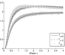
Figure 3. Final thresholds for the 7 peeling algorithms for $u=[0.1\dots 4]$. For comparison, universal threshold $T_{u}=4.29$ for $N=10000$.

4.2. Denoising: simulated signals

To assess the denoising performances of the peeling algorithm, we used the 4 classical benchmarks proposed in [6], namely Blocks, Bumps, HeaviSine, Doppler (figure 4), with 4 lengths ($N=[2048,4096,8192,16384]$). The signals were normalized to have unitary power. Twenty types of zero-mean random noise $n$ were generated according to generalized gaussian with shape parameters $u_{n}=[0.2,0.4,0.6\dots 3.8,4]$. The noise was then scaled to obtain signal to noise ratios $SNR=[1,2,3]$, i.e., [ 0, 3, 4.8] decibels. Furthermore, the wavelet decomposition of the signal has been performed based on the sym 8 wavelet, and the noise was added to the wavelet coefficients of the noise-free signals to obtain the “measured signal” wavelet coefficients $z$. Each of these noisy signals were simulated 500 times to obtain averaged results. A statistical hypothesis testing showed that the wavelet coefficient of the signals under consideration could be assimilated to generalized Gaussian random variables, with the notable exception of the Bumps process.

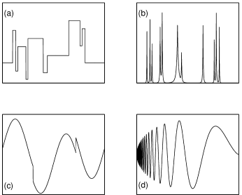
Figure 4. Benchmark signals: (a) Blocks, (b) Bumps, (c) HeaviSine,, (d) Doppler

The shape parameter $u_{z}$ of the total signal $z$, which determines the thresholds of the peeling algorithms, was estimated using the absolute empirical moments $m_{1}$ and $m_{2}$, (with $m_{r}=\mathds{E}[|z|^{r}]$, see [11, 10]), while the mean $\mu_{z}$ and the standard deviation $\sigma_{z}$ were estimated using classical empirical estimators.

Denoising was performed by soft thresholding (instead of the hard one described by equation (3)) using the 7 algorithms described at Section 4.1, as well as the classical Universal and SURE thresholding [6], for comparison. More elaborated wavelet denoising methods (either based on redundant wavelet transforms or on block approaches [3, 17, 18]) were not considered for the comparison, since their nature is different: all the algorithms tested in this paper are term-by-term approaches for orthogonal wavelet transform thresholding.

The denoised estimate $\hat{x}$ of the original signal was reconstructed by inverse wavelet transform. We recall here that Universal thresholding aims to completely eliminate Gaussian noise (and therefore it risks to distort the signal), while SURE thresholding estimates the original signal my minimizing the Stein Unbiased Risk Estimator of the mean squared error between $x$ and $\hat{x}$, assuming also a Gaussian noise (thus basically aiming a minimum distortion of the signal, as the peeling algorithms). The denoising performance was evaluated using the signal to noise ratio after denoising:

$$SNR_{den}=10\log_{10}\frac{\sum_{i=1}^{N}(x(i))^{2}}{\sum_{i=1}^{N}(x(i)-\hat{x}(i))^{2}}$$

As expected, the results obtained for $\hat{T}_{c,05}$, $\hat{T}_{c,15}$, $\hat{T}_{cm}$ and $T_{m}$ are very similar to those obtained by ${T}_{c,05}$, ${T}_{c,15}$, ${T}_{cm}$, so only results of the three latter are detailed here . Synthetic comparisons are presented at Figure 5 for different shape parameters $u_{n}$ of the noise distribution, for all the 4 benchmark signals and for $N=4096$ (to ease the presentation, detailed tables of results are omitted, since the values can be read with enough precision on the graphs).

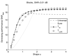
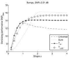
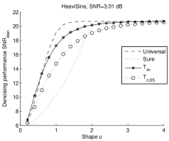
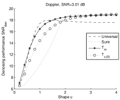
Figure 5. Signal to noise ratios after denoising as a function of the noise distribution. The presented graphs are obtained for noisy signals with $SNR$=3dB.

An illustrative example on the Block signal is also provided at Figure 6.

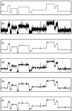
Figure 6. Denoising example for $Blocks$: (a) original signal, (b) noisy signal (Laplacian noise $u_{n}$=1, $SNR$=10dB), (c) Universal ($SNR_{den}$=17.7dB), (d) SURE ($SNR_{den}$=16.9dB), (e) $T_{c,05}$ ($SNR_{den}$=18.6dB), (f) $T_{cm}$ ($SNR_{den}$=18.5dB)

Several interesting observations can be made. Obviously, the noise type (shape parameter $u_{n}$) greatly influences the performances of all algorithms: they are lower for heavy-tailed noise distributions, which indicates that this type of noise is more difficultly eliminated from measured signals. As one could expect from its development, SURE thresholding is the best choice for Gaussian noise, for which it also attains its best performance (this algorithm continue to have a very good performance for higher $u_{n}$). The Universal thresholding attains its best performance for Laplacian noise $u=1$ and it has very good results for super-Gaussian noises ($u_{n}<2$). On the contrary, its performances are the worst for high values of the shape parameter of the noise (except for the very low frequency signal HeaviSine, for which all algorithms are similar for sub-Gaussian noises $u_{n}>2$).

The peeling algorithms need a more detailed analysis: they are better than SURE for super-Gaussian noises, with the theoretical $T_{c,15}$ (or, equivalently, theoretical $T_{cm}$ and iterative $\hat{T}_{cm}$, $\hat{T}_{c,15}$ and $T_{m}$) being slightly better than $T_{c,0.5}$. The order between the two peeling algorithms tend to change for sub-Gaussian noise ($u_{n}>2$), especially for impulsive Blocks and Bumps. To conclude, it seems that for super-Gaussian noises, Universal thresholding and peeling algorithms are the best choice, while for sub-Gaussian noises the results are almost similar, with SURE thresholding having the best performances when the noise is almost Gaussian. In all, the peeling algorithm with $T_{c,15}$ works in a satisfying way, independently of the shape parameter $u$.

4.3. Denoising: real and pseudo-real signals

A last point should be reminded: peeling algorithms were mainly developed for biomedical applications [4, 9]. Therefore, we have chosen to evaluate the performance of the newly developed versions on biological signals (normal electrocardiogram – ECG and normal background electroencephalogram EEG). However, when dealing with real signals for denoising, one is faced with the following problem: it is impossible to assert that the denoising is accurate when the original signal is unknown. It is also very hard to be provided with a non noisy signal which can be perturbed artificially.

In order to cope with this situation, we have chosen to work with a commonly used ECG simulator, implemented in Matlab. In this way, one can produce a clean ECG type signal, spoil it with an artificial noise, and then try to recover the original signal by some denoising procedures. The simulated EEG was generated according to the procedure described in [19] (see the url for the Matlab code).

This is the protocol we have followed for our experiment. Numerical results globally confirm those obtained on the benchmark signals, both for the simulated ECG and EEG. They are not reproduced here for sake of conciseness, but an illustrative example is given at Figure 7.

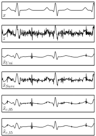
Figure 7. Denoising example for a simulated $ECG$: $x$ original signal, $z$ noisy signal (Laplacian noise $u_{n}$=1, $SNR$=0dB), $\hat{x}_{Uni}$ Universal thresholding ($SNR_{den}$=4.8dB), $\hat{x}_{Sure}$ Sure thresholding ($SNR_{den}$=3.7dB), $\hat{x}_{c,05}$ $T_{c,05}$ thresholding ($SNR_{den}$=5.9dB) and $\hat{x}_{c,15}$ $T_{c,15}$ thresholding ($SNR_{den}$=5.3dB).

Two-dimensional versions of the tested algorithms were applied on real benchmark images also ($Lena$, $House$, $Barbara$, $Peppers$), with similar performances to those obtained for the 1-D signals. Therefore, the detailed results are not presented here.

References

- [1] A. Antoniadis, J. Bigot, T. Sapatinas: Wavelet estimators in non-parametric regression: a comparative simulation study. Preprint, 2006.
- [2] C. Chesneau: Wavelet block thresholding for samples with random design: a minimax approach under the risk. Electron. J. Stat. 1 (2007), 331–346.
- [3] R. Coifman, D. Donoho: Translation invariant denoising. Wavelets and Statistics, ed. A. Antoniadis and G. Oppenheim, Springer Verlag, 125-150 (1995).
- [4] R. Coifman, M. Wickerhauser: Adapted waveform de-noising for medical signals an images, IEEE Engineering in Medecine and Biology Magazine 14, no. 5, 578-586 (1995).
- [5] I. Daubechies: Ten lectures on wavelets. Society for Industrial and Applied Mathematics (1992).
- [6] D. Donoho, I. Johnstone: Ideal spatial adaptation via wavelet shrinkage. Biometrika 81, 425-455 (1994).
- [7] D. Donoho, I. Johnstone, G. Kerkyacharian, D. Picard: Wavelet shrinkage: asymptopia? With discussion and a reply by the authors. J. Roy. Statist. Soc. Ser. B 57, no. 2, 301–369 (1995).
- [8] E. Giné, R. Nickl: Uniform limit theorems for wavelet density estimators. Ann. Probab. 37, no. 4, 1605–1646 (2009).
- [9] L. Hadjileontiadis, S. Panas: Separation of discontinuous adventitious sounds from vesicular sounds using a wavelet based filter. IEEE Transactions on Biomedical Engineering 44, no. 12, 1269-1281 (1997).
- [10] K. Kokkinakis, A. Nandi: Exponent parameter estimation for generalized Gaussian probability density functions with application to speech modeling. Signal Processing 85, 1852-1858 (2005).
- [11] S. Mallat: A Theory for Multiresolution Signal Decomposition: The Wavelet Representation. IEEE Transactions on Pattern Analysis and Machine Intelligence 11, no. 7, 674-693 (1989).
- [12] S. Mallat: A wavelet tour of signal processing. Academic Press (1997).
- [13] A. Pizurica, V. Zlokolica, and W. Philips: Noise reduction in video sequences using wavelet-domain and temporal filtering, in SPIE Conference Wavelet Applications in Industrial Processing, Providence, Rhode Island, USA (2003).
- [14] R. Ranta, C. Heinrich, V. Louis-Dorr, D. Wolf: Interpretation and improvement of an iterative wavelet-based denoising method. IEEE Signal Processing Letters 10, no. 8, 239-241 (2003).
- [15] R. Ranta, C. Heinrich, V. Louis-Dorr, D. Wolf: Iterative wavelet-based denoising methods and robust outlier detection. IEEE Signal Processing Letters 12, no. 8, 557-560 (2005).
- [16] A. van der Vaart, J. Wellner: Weak convergence and empirical processes, Springer (1996).
- [17] T. Cai, B. Silverman: Incorporating information on neighbouring coefficients into wavelet estimation,Sankhyā: The Indian Journal of Statistics. Special issue on Wavelets 63, no. 2, 127-148 (2001).
- [18] T. Cai, H. Zhou: A Data-Driven Block Thresholding Approach to Wavelet Estimation, The Annals of Statistics, to appear, http://www-stat.wharton.upenn.edu/ tcai/Papers.html
- [19] L. Rankine, N. Stevenson, M. Mesbah, B. Boashash: A Nonstationary Model of Newborn EEG, IEEE Transactions on Biomedical Engineering 54, no. 1, 19-28 (2007), http://www.som.uq.edu.au/research/sprcg/newborn.asp