Dynamic response of a mesoscopic capacitor in the presence of strong electron interactions

Abstract

We consider a one dimensional mesoscopic capacitor in the presence of strong electron interactions and compute its admittance in order to probe the universal nature of the relaxation resistance. We use a combination of perturbation theory, renormalization group arguments, and quantum Monte Carlo calculation to treat the whole parameter range of dot-lead coupling. The relaxation resistance is universal even in the presence of strong Coulomb blockade when the interactions in the wire are sufficiently weak. We predict and observe a quantum phase transition to an incoherent regime for a Luttinger parameter $K<1/2$. Results could be tested using a quantum dot coupled to an edge state in the fractional quantum Hall effect.

The dynamical response of mesoscopic conductors constitutes a mostly unexplored area of coherent quantum transport, which has recently led to groundbreaking experiments gabelli . The mesoscopic capacitor buttiker_pretre is one of its elementary building blocks: a quantum dot influenced by an AC gate voltage, which is put in contact with an electron reservoir. It has been studied so far at the single electron level, with possible mean field generalizations nigg . Both the capacitance $C_{\mu}$ and the relaxation resistance $R_{q}$, obtained from the low frequency expansion of the admittance $G(\omega)\approx-i\omega C_{\mu}+\omega^{2}C_{\mu}^{2}R_{q}$, are fundamentally affected by the quantum coherence of the device. At zero temperature, a single spin polarized channel yields a relaxation resistance $R_{q}=h/(2e^{2})$, which is independent of the dot-reservoir connection. Ref. gabelli has confirmed this result for a quantum dot with weak charging energy.

However, quantum dots with reduced size exhibit strong Coulomb blockade, and there is also a clear need to analyze whether electron-electron interactions in the lead are relevant. Here, taking rigorously these aspects into account, we prove that there is quantum phase transition from a coherent to an incoherent regime, where a relaxation resistance cannot be defined. For weak interactions, the universal behavior is recovered even in the presence of strong Coulomb blockade.

We consider a quantum dot (Fig. 1) connected to a reservoir modelled by a Luttinger liquid lead, which allows to account exactly for Coulomb blockade effects. We discuss separately the absence (Luttinger parameter $K=1$) or the presence ($K<1$) of interaction in the adjacent lead. This setup and the underlying physics is similar to that studied in Ref. Furusaki02 , where attention was solely focused on the static occupation of a resonant level. Here we show that below $K=1/2$ the Kosterlitz Thouless type phase transition driven by the dot-lead tunneling strength triggers a transition of dynamical transport from a coherent to an incoherent regime, hence provoking a deviation from the universal $R_{q}=h/(2e^{2})$. We use a combination of analytical (perturbation theory, renormalization group) and numerical (quantum Monte Carlo) approaches to monitor the capacitance and the relaxation resistance over the whole range of dot-lead connection. The present results can be applied to carbon nanotube quantum wires as well as dots defined in the fractional quantum Hall effect (FQHE).

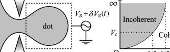
Figure 1: Left: schematic view of the mesoscopic capacitor: a 1D quantum dot, capacitively coupled to a gate with time-dependent voltage $V_{g}+\delta V_{g}(t)$. Right: schematic phase diagram in the degenerate case. $V_{c}$ denotes the critical backscattering strength for $K=1/3$.

The starting point is the Hamiltonian for a non-chiral, semi-infinite Luttinger liquid kane_fisher_92 where the dot region corresponds to the interval $[0,L]$:

$$H= \int_{-\infty}^{L}\frac{{\rm d}x}{2\pi}\left[\frac{v_{F}}{K^{2}}\left(\frac{\partial\phi}{\partial x}\right)^{2}+v_{F}\left(\frac{\partial\theta}{\partial x}\right)^{2}\right]-V\cos[2\phi(x=0)]$$

$$+\frac{1}{\pi^{2}}E_{C}\left[\phi(x=0)-\left(\frac{\pi CV_{g}}{|e|}+k_{F}L\right)\right]^{2}.$$ (1)

The first part is the kinetic part, followed by the backscattering term at $x=0$ (strength $V$), and finally the contribution from the charging energy with $E_{C}\equiv e^{2}/(2C)$ ($C$ is the geometrical capacitance). The canonically conjugated fields $\phi$ and $\theta$ satisfy the commutation relation $[\phi(x),\theta(x^{\prime})]=(i\pi/2)\mbox{sgn}(x-x^{\prime})$. $V$ is the backscattering strength on the point contact. $E_{C}\equiv e^{2}/(2C)$ denotes the charging energy The time dependent gate voltage oscillates around $V_{g}$. Using the Matsubara imaginary time path integral formulation, the quadratic degrees of freedom away from $x=0$ can be integrated out. The kinetic part of the effective action then reads $S_{kin}=(\pi K\beta)^{-1}\sum_{\omega_{n}}|\omega_{n}|/(1-{\rm e}^{-2\pi K|\omega_{n}|/\Delta})|\tilde{\phi}(\omega_{n})|^{2}$, where $\tilde{\phi}(\omega_{n})$ is the Fourier transform of $\phi(\tau)$ (now specified at $x=0$), and $\Delta\equiv\pi v_{F}/L$ is the level spacing. The same action can be derived alternatively starting from a single chiral Luttinger liquid “loop”, hence the relevance for the FQHE regime FQHE_explain . Within linear response in the oscillating gate voltage, the (imaginary frequency) admittance can be expressed as:

$$G(i\omega_{n})=\frac{e^{2}}{h}\frac{2|\omega_{n}|}{\pi}\int_{0}^{\beta}{\rm d}\tau\langle\phi(\tau)\phi(0)\rangle{\rm e}^{i\omega_{n}\tau}.$$ (2)

The dynamical conductance is obtained by analytic continuation $G(\omega)=G(i\omega_{n}\rightarrow\omega+i\delta$), while the capacitance reads:

$$C_{\mu}=\frac{e^{2}}{\pi^{2}}\beta[\langle\bar{\phi}^{2}\rangle-\langle\bar{\phi}\rangle^{2}]\qquad\left(\bar{\phi}\equiv\frac{1}{\beta}\int_{0}^{\beta}{\rm d}\tau\phi(\tau)\right).$$ (3)

We start with a discussion of the weak barrier case, using perturbation theory in $V/D$ (bandwidth $D$). The capacitance and relaxation resistance are derived as an expansion in orders of $V$, $C_{\mu}=C_{\mu}^{(0)}+C_{\mu}^{(1)}+C_{\mu}^{(2)}+...$ and $R_{q}=R_{q}^{(0)}+R_{q}^{(1)}+R_{q}^{(2)}+...$. Introducing

$$a_{n}=\frac{1}{\pi K\beta}\left(\frac{|\omega_{n}|}{1-{\rm e}^{-2\pi K|\omega_{n}|/\Delta}}+\frac{E_{C}K}{\pi}\right),$$ (4)

one obtains to zeroth, first and second order:

$$G^{(0)}(i\omega_{n}) =\frac{e^{2}}{h}\frac{|\omega_{n}|}{\pi}\frac{1}{\beta a_{n}}$$ (5)

$$G^{(1)}(i\omega_{n}) =-\frac{e^{2}}{h}\frac{|\omega_{n}|}{\pi}2V\sqrt{F_{+}(0)}\frac{1}{\beta^{2}a_{n}^{2}}\cos(2\pi N)$$ (6)

$$G^{(2)}(i\omega_{n}) =\frac{e^{2}}{h}\frac{|\omega_{n}|}{\pi}2V^{2}F_{+}(0)\frac{1}{\beta^{2}a_{n}^{2}}I(\omega_{n}),$$ (7)

where we defined:

$$F_{\pm}(v)=\exp\left[-\sum_{n}\frac{\pm 2}{\beta^{2}a_{n}}\cos(\omega_{n}v)\right]$$ (8)

$$I(\omega_{n})=\int_{0}^{\beta/2}{\rm d}v\left[\cos(4\pi N)V_{+}(\omega_{n},v)+V_{-}(\omega_{n},v)\right]$$ (9)

$$V_{\pm}(\omega_{n},v)=1-F_{\pm}(v)\left(1\pm\cos(\omega_{n}v)\right)$$ (10)

$$N=\frac{k_{F}L}{\pi}+\frac{|e|V_{g}}{2E_{T}}\quad\mbox{with}\quad E_{T}=E_{C}+\frac{\Delta}{2K^{2}}.$$ (11)

The $\sum_{n}$ in $F_{\pm}$ is limited by $D$. From Eqs. (5)-(7), the capacitance at low temperature becomes:

$$C^{(0)}_{\mu} =\frac{e^{2}}{h}\frac{\pi}{E_{T}}$$ (12)

$$C^{(1)}_{\mu} =-C^{(0)}_{\mu}\frac{\pi^{2}}{E_{T}}2V\sqrt{F_{+}(0)}\cos(2\pi N)$$ (13)

$$C^{(2)}_{\mu} =C^{(0)}_{\mu}\frac{\pi^{2}}{E_{T}}2V^{2}F_{+}(0)I(\omega_{n}\rightarrow 0)\cos(4\pi N).$$ (14)

It is clear from these expressions that the total capacitance $C_{\mu}$ is a periodic function of $N$, with period 1. Below we focus on the interval $0\leq N<1$. The results for the relaxation resistance, at low temperature, are simple since the computation of the first and second order contribution shows that they vanish:

$$R_{q}^{(0)}+R_{q}^{(1)}+R_{q}^{(2)}=R_{q}^{(0)}=\frac{h}{2e^{2}}\frac{1}{K}.$$ (15)

The charging energy thus does not modify the value of relaxation resistance, while electron interactions in the lead introduce a trivial factor $1/K$. At zero temperature, the sums and integration of Eqs. (5)-(7) can be done analytically in certain cases. For example, when $E_{C}=0$ and $K=1$, one has $F_{+}(0)=(\Delta/(2\pi D))^{2}$ ($D\gg\Delta$), and one can show that the result for the capacitance is $C_{\mu}=(e^{2}/\Delta)(1-2r\cos(2\pi N)+2r^{2}\cos(4\pi N))$, with $r=\pi V/D$. This coincides with the development of the non-interacting formula found in Ref. [gabelli, ] in powers of the reflection coefficient $r$: $C_{\mu}=(e^{2}/\Delta)(1-r^{2})/(1-2r\cos(2\pi N)+r^{2})$. In the more general case of non-zero $E_{C}$, and $K\neq 1$, one has $F_{+}(0)\sim(E_{T}K/(\pi D))^{2K}$, and the integration of Eq. (7) has to be computed numerically.

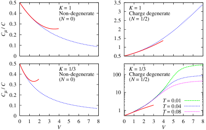
Figure 2: (color online) Capacitance $C_{\mu}$ as a function of the backscattering strength $V$, obtained at temperature $T=0.04$ with Monte Carlo computations (dashed lines). The solid lines show the predictions of the perturbative calculations up to second order. We take $E_{C}/\pi^{2}$ as the unit of energy and use the parameters $D\equiv 2\pi J/\beta=8\pi$ and $\Delta/(2K^{2})=\pi^{2}$. Temperature dependence is shown in the bottom right panel, where the vertical axis is measured on a logarithmic scale.

The perturbation theory thus proves the universality of the charge relaxation resistance in the weak barrier limit even in the presence of interactions. To study the non-perturbative regime, the path-integral Monte Carlo method is applied to the action for the discretized path $\phi(\tau=j\beta/J)$ $(j=0,1,\cdots,J-1)$. We estimate thermal average by generating discretized paths using local update in the Fourier space and the cluster update Werner05 ; Hamamoto . The top (bottom) row of Fig. 2 shows the calculated capacitance $C_{\mu}$ as a function of $V$ at $T=0.04$ and $K=1$ ($K=1/3$). The left and right columns correspond to the non-degenerate case ($N=0$) and the charge degenerate case ($N=1/2$), respectively. With increasing $V$ the Coulomb staircase becomes sharper, which results in the decrease (increase) in $C_{\mu}\equiv\partial\langle Q\rangle/\partial V_{g}$ in the case of $N=0$ ($N=1/2$). The second-order perturbation theory, shown as solid lines, displays an excellent agreement for small $V$. Especially, it is remarkable that only for the case of $K=1/3$ and $N=1/2$ (the right bottom panel of Fig. 2), $C_{\mu}$ exhibits an abrupt increase at a finite $V$, signaling a possible transition. One can see that $C_{\mu}$ grows as $\propto 1/T$ in the large barrier region.

To reveal the origin of the transition behavior, we next examine the strong barrier limit using an instanton method which was developed for the Kondo model anderson . Near the degeneracy point $N=1/2$, the configuration of the bosonic field $\phi$ can be represented in the dilute instanton gas approximation

$$\phi(\tau)\simeq\pi\sum_{j=1}^{2n}s_{j}\Theta(\tau-\tau_{j})+\frac{\pi}{2}(1-s),$$ (16)

where $s_{j}=s(-1)^{j-1}$, and $s\sim 1$ denotes the separation between the well minima ($\Theta$ is the step function). Inserting Eq. (16) in the full effective action, the partition function becomes:

$$\begin{split}Z&=\sum_{n=0}^{\infty}t^{2n}\int_{0}^{\beta}{\rm d}\tau_{2n}\int_{0}^{\tau_{2n}}{\rm d}\tau_{2n-1}\cdots\int_{0}^{\tau_{2}}{\rm d}\tau_{1}\\ &\phantom{=}\times\exp\left[\frac{1}{2K}\sum_{j\neq k}s_{j}s_{k}\log\frac{|\tau_{j}-\tau_{k}|}{\tau_{c}}-u\sum_{j}s_{j}\tau_{j}\right],\end{split}$$ (17)

where $t$ is the tunneling amplitude between the well minima, and $\tau_{c}$ is the short-time cutoff. $u=(2N-1)E_{T}$ denotes the deviation from the degeneracy point. Note the similarity between this partition function and that which was proposed in the context of dissipative Josephson junctions chakravarty . One can therefore identify the scaling equations :

$$\frac{{\rm d}t}{{\rm d}l}=\left(1-\frac{s^{2}}{2K}\right)t,\quad\frac{{\rm d}s^{2}}{{\rm d}l}=-4s^{2}t^{2},$$ (18)

$$\frac{{\rm d}us}{{\rm d}l}=us(1-2t^{2})$$ (19)

which are familiar in the context of a Kosterlitz Thouless transition in the two-dimensional XY model. No further arguments are needed when one deviates from the degeneracy point: since $t$ is small, starting from $u\neq 0$, Eq. (19) predicts that $u$ will further increase, leading the system further away from the degeneracy point. This means that $\phi$ will be trapped in an effective harmonic potential, and one thus recover the result of Eq. (5), which is therefore universal. For the charge degenerate case $N=1/2$, the transition corresponds to a Kondo type transition associated with the charge pseudo spin on the dot. Eqs. (18) determine the tendency of the dot-lead transmission as temperature is lowered; $(t,s^{2})$ flows along one of the hyperbolic curves $B^{2}-4t^{2}={\rm const}.$, where $B\equiv 1-s^{2}/(2K)$. For $K>1/2$, the tunneling strength always grows upon reducing the temperature, and the system reaches the Kondo fixed point where the dot is strongly coupled to the reservoir. An electron freely tunnels in and out of the dot irrespective of the initial tunneling strength. In particular at $K=1$ this implies that the charge relaxation resistance is universal, i.e., $R_{q}=h/(2e^{2})$, as a consequence of the unitary limit of the underlying Kondo model. On the other hand for $K<1/2$, there is the possibility that at a critical, sufficiently weak transmission $t$ (“large” $V$), the RG flow always drives the system into a weak coupling configuration with specified charge. Then the charge fluctuation remains finite, i.e., $\langle\bar{\phi}^{2}\rangle-\langle\bar{\phi}\rangle^{2}\simeq(\pi s/2)^{2}$, so that the capacitance diverges as $\propto 1/T$ at low temperatures [see Eq. (3)]. This explains the transition observed for the capacitance in the strongly interacting case.

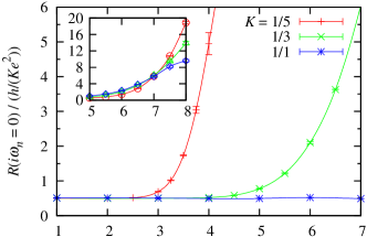
Figure 3: (color online) Extrapolated value $R(i\omega_{n}\rightarrow 0)$ as a function of $V$ at temperature $T=0.04$ in the degenerate case. For $D$ and $\Delta/(2K^{2})$, we use the same parameters as in Fig. 2. Inset: $R(i\omega_{n}\rightarrow 0)$ for $K=1/3$ at $T=0.01(\circ)$, $0.04(\triangle)$ and $0.08(\diamond)$ in the vicinity of the location where the crossing occurs.

We now describe the effect of the KT transition on the dynamical properties. If $\omega\ll 1/\tau_{RC}$ holds (with $RC$ time $\tau_{RC}$), the charge relaxation resistance can be defined in the low-frequency expansion $G(\omega)=-i\omega C_{\mu}+\omega^{2}C_{\mu}^{2}R_{q}+\mathcal{O}(\omega^{3})$. However, the validity of this expansion is not obvious, since the KT transition may influence $\tau_{RC}$ itself. Instead, we investigate the low-frequency resistance using

$$R(i\omega_{n})\equiv\frac{1}{G(i\omega_{n})}-\frac{1}{\omega_{n}C_{\mu}},$$ (20)

where $G(i\omega_{n})$ and $C_{\mu}$ are defined in Eqs. (2) and (3), respectively. The extrapolation $R(i\omega_{n}\rightarrow 0)$ gives the real part of the impedance in the low-frequency limit, hence $\tau_{RC}=R(0)C_{\mu}$. In Fig. 3, we plot $R(0)$ for $K=1,1/3$ and $1/5$ as a function of $V$ at temperature $T=0.04$. For $K=1$, $R(0)$ equals $h/(2e^{2})$ irrespective of $V$, in agreement with the universal charge relaxation resistance buttiker_pretre ; nigg . For $K=1/3$ and $1/5$, the universality is observed in the weak barrier region, whereas $R(0)$ is abruptly enhanced with increasing $V$, reflecting the RG flow to the weak coupling regime due to the KT transition. The temperature dependence of $R(0)$ for $K=1/3$ is shown in the inset of Fig 3, which indicates that $R(0)$ diverges as $T\rightarrow 0$ in the strong barrier region.

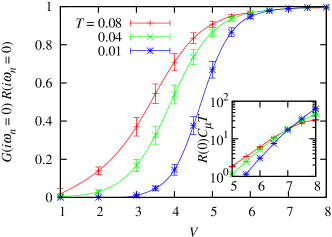
Figure 4: (color online) Product $G(i\omega_{n}=0)R(i\omega_{n}=0)$ for $K=1/3$ as a function of the backscattering strength $V$, for different temperatures $T$. For $D$ and $\Delta/(2K^{2})$, we use the same parameters as in Fig. 2. Inset: $R(0)C_{\mu}T$ as a function of $V$, for different $T$; the crossing of the curves gives a good estimate of the transition point.

The KT transition plays a crucial role in the relevance of the universal charge relaxation resistance. If $2t+B>0$, the system scales to the weak barrier limit, where $\tau_{RC}$ is independent of temperature. If $2t+B<0$, on the other hand, the scaling equations (18) predict $s^{2}\rightarrow{\rm const.}$ and $t\propto T^{-B}$, so that $\tau_{RC}$ roughly scales as $\propto T^{-1}(T^{2B}+{\rm const.})$, which grows faster than the (thermal) coherence time $\tau_{\rm coh}\propto 1/T$ as temperature is lowered. These observations suggest that if $2t+B>0$ coherent transport can be realized by lowering temperature to guarantee $\tau_{RC}<\tau_{\rm coh}$, while if $2t+B<0$ electronic transport in the dot decoheres before charge relaxation is achieved. In the latter case, the quantum dot effectively acts as a reservoir and consequently the dynamical property of the system is governed by transport through the point contact between the two “reservoirs”. Therefore the $V$-dependent low-frequency resistance observed in the inset of Fig. 3 reflects the revival of the Landauer-type transport. To see this behavior more clearly, we plot in Fig. 4 the product $G(i\omega_{n}\rightarrow 0)R(i\omega_{n}\rightarrow 0)$ for $K=1/3$ as a function of $V$. In the strong barrier region, $G(0)$ is finite and equal to $[R(0)]^{-1}$, which is a familiar property of transport through a point contact. Upon decreasing $V$, however, $G(0)R(0)$ is suppressed since $G(0)$ decays to zero because of charging up, although $R(0)\rightarrow R_{q}$ is finite. Moreover, we see that the coherent region $G(0)R(0)=0$ extends to larger $V$ upon lowering temperature. Finally, we determine the phase boundary of the coherent-incoherent transition by tracing the temperature dependence of the ratio $\tau_{RC}/\tau_{\rm coh}=R(0)C_{\mu}T$. The above discussion suggests that there exists a critical backscattering strength $V_{c}$, below which $\tau_{RC}/\tau_{\rm coh}$ decays to zero, while it diverges otherwise (see the right panel in Fig. 1). From the inset of Fig. 4, the critical value is estimated as $V_{c}\simeq 7$.

In conclusion, the study of the mesoscopic capacitor in the presence of strong electron electron interaction shows that the relaxation resistance for a dot connected to Luttinger liquid is universal $R_{q}\equiv h/(2e^{2}K)$ as long as interactions are sufficiently weak. Below $K<1/2$, this resistance is governed by the strength of the dot-lead coupling: at the charge degeneracy point, there is a critical coupling strength, governed by a KT type phase transition, below which the dot acts as an incoherent reservoir and the low-frequency resistance exceeds the universal value. In this incoherent regime, the charge relaxation resistance cannot be defined anymore due to the divergence of the $RC$ time.

Results could be probed experimentally using quantum dots connected to an edge state in the FQHE regime. Another experimental probe could use one dimensional quantum wires (non chiral Luttinger liquids) with the limitation that the operating frequency would have to be larger than the inverse time of flight within the wire, in order to avoid renormalization effects due to eventual Fermi liquid leads connected to this wire maslov_stone .

Y.H. and T.K. are grateful to T. Fujii for valuable discussions. Y.H. acknowledges the support of the Japan Society for the Promotion of Science. This research was partially supported by JSPS and MAE under the Japan-France Integrated Action Program (SAKURA) and by Grant-in-Aid for Young Scientists (B) (No. 21740220) from the Ministry of Education, Science, Sports and Culture. It was also supported by ANR-PNANO Contract MolSpinTronics, No. ANR-06-NANO-27. The computation in this work was done using the facilities of the Supercomputer Center, Institute for Solid State Physics, University of Tokyo.

References

- (1) J. Gabelli, G. Feve, J.-M. Berroir, B. Plaçais, A. Cavanna, B. Etienne, Y. Jin, and D. C. Glattli, Science 313, 499 (2006); J. Gabelli, G. Feve, T. Kontos, J.-M. Berroir, B. Plaçais, D.C. Glattli, B. Etienne, Y. Jin, M. Büttiker, Phys. Rev. Lett. 98, 166806 (2007).
- (2) M. Büttiker, H. Thomas, and A. Prêtre, Phys. Lett. A 180, 364 (1993).
- (3) S. E. Nigg, R. López, and M. Büttiker, Phys. Rev. Lett. 97, 206804 (2006).
- (4) A. Furusaki and K. A. Matveev, Phys. Rev. Lett. 88, 226404 (2002).
- (5) C. L. Kane and M. P. A. Fisher, Phys. Rev. Lett. 68, 1220 (1992); A. Furusaki and N. Nagaosa, Phys. Rev. B, 47, 3827 (1993).
- (6) In the FQHE regime, denotes the strength of quasi-particle tunneling.
- (7) P. Werner and M. Troyer, Phys. Rev. Lett. 95, 060201 (2005).
- (8) Y. Hamamoto, K.-I. Imura, and T. Kato, Phys. Rev. B 77, 165402 (2008); Y. Hamamoto and T. Kato, ibid. 77, 245325 (2008).
- (9) P. W. Anderson, G. Yuval, and D. R. Hamann, Phys. Rev. B 1, 4464 (1970).
- (10) S. Chakravarty, Phys. Rev. Lett. 49, 681 (1982).
- (11) D. L. Maslov and M. Stone, Phys. Rev. B 52, R5539 (1995).