Second order QCD corrections to inclusive semileptonic $b\to X_{c}l\bar{\nu}_{l}$ decays with massless and massive lepton

Abstract:

We extend previous computations of the second order QCD corrections to semileptonic $b\to c$ inclusive transitions, to the case where the charged lepton in the final state is massive. This allows accurate description of $b\to c\tau\bar{\nu}_{\tau}$ decays. We review techniques used in the computation of ${\cal O}(\alpha_{s}^{2})$ corrections to inclusive semileptonic $b\to c$ transitions and present extensive numerical studies of ${\cal O}(\alpha_{s}^{2})$ QCD corrections to $b\to cl\bar{\nu}_{l}$ decays, for $l=e,\tau$.

1 Introduction

Inclusive semileptonic decays of $B$-mesons into charmed final states $B\to X_{c}l\bar{\nu}_{l}$ are benchmark processes in $B$-physics. These processes were studied extensively at $B$-factories, LEP and the Tevatron [1, 2, 3, 4, 5, 6]. When lepton in the final state is electron or muon, most of the experimental data come from BABAR and BELLE, while measurements of inclusive rate for $b\to X_{c}\tau\bar{\nu}_{\tau}$ transition are due to ALEPH and OPAL [7, 8]. At $B$-factories only preliminary results on exclusive decay $B\to D\tau\bar{\nu}_{\tau}$ were reported [9].

Theoretically, inclusive semileptonic decays of $B$-mesons are well-understood, thanks to the Operator Product Expansion (OPE) in inverse powers of the $b$-quark mass [10]. When results of experimental measurements for $B\to X_{c}l\bar{\nu}_{l}$ are compared with theoretical predictions, one is able to determine with high precision the bottom and charm quark masses, the CKM matrix element $|V_{cb}|$ and the non-perturbative parameters of the heavy quark expansion [11, 12, 13]. Measurements of $\tau$ lepton branching fractions by ALEPH and OPAL are used to constrain possible contributions of a charged Higgs boson to semileptonic $B$-decays.

An important issue in physics of semileptonic $B$-decays, intimately related to a very high precision achieved in experimental measurements, and the intention to utilize this precision fully, is the necessity to understand and control perturbative QCD corrections in heavy quark decays. There are two aspects of this problem. First, one needs to understand the general structure of these corrections, to avoid large perturbative effects. A by-now standard example of this type is the recognition of a special role that short-distance low-scale quark masses play in avoiding large perturbative effects in quark decays [14]. Second, it is very important to provide explicit computations of QCD radiative corrections to quantities of direct relevance for experimental analysis. Large number of experimental results comes in the form of moments of lepton energy, hadron energy and hadron invariant mass with variable cut on the lepton energy. These are sufficiently complicated observables to make analytic computations, in particular in higher orders, impractical. On the contrary, if QCD effects are computed numerically for fully differential decay rates, any restriction on final state particles can be imposed.

It is interesting to point out in this regard that, while one-loop corrections to the decay rate and a number of basic differential distributions for $b\to X_{c}l\bar{\nu}_{l}$ decays were computed long ago [15, 16], fully differential decay rate through ${\cal O}(\alpha_{s})$ was obtained only in 2004 [17, 18, 19]. Early estimates of two-loop QCD corrections to the total rate for $b\to X_{c}e\bar{\nu}_{e}$ decays were given in Refs. [20, 21, 22]. Fully differential decay rate through ${\cal O}(\alpha_{s}^{2})$ for $b\to X_{c}e\bar{\nu}_{e}$ was computed very recently in Ref. [23]. That calculation is based on the techniques developed in Refs. [24] for the computation of next-to-next-to-leading order (NNLO) QCD corrections to a number of processes in hadron collider physics. Those techniques were first applied to describe weak decays of charged fermions in Ref. [25], where two-loop QED corrections to the electron energy spectrum in muon decay were studied. We note that analytic results for semileptonic decay rate $b\to X_{c}l\bar{\nu}_{l}$ and moments of the lepton energy without lepton energy cut were computed through ${\cal O}(\alpha_{s}^{2})$ in the form of $m_{c}/m_{b}$ expansion in Refs. [26, 27]. Analytic results reported in those references are very handy – especially, when compared to numerical calculations reported in Ref. [23] and in the current paper – but it is not clear a’priori if they can be used for moments with lepton energy cuts, because the precision achieved in experimental measurements is rather high. Finally, we note that efforts are underway to compute ${\cal O}(\alpha_{s})$ corrections to Wilson coefficients of leading non-perturbative operators, that contribute to moments in $b\to X_{c}l\bar{\nu}_{l}$ transitions [28].

There are two goals that we pursue in this paper. First, we extend the calculation reported in Ref. [23] by considering massive lepton in the final state. Once this is accomplished, we have a fully differential description of $b\to X_{c}l\bar{\nu}_{l}$ transition, where $l$ can be electron, muon or $\tau$. Second, we present a much more detailed study of ${\cal O}(\alpha_{s}^{2})$ corrections in semileptonic $B$-decays, than what was published in Ref. [23].

We point out that since our computations are numerical, the presence of a massive lepton in the final state is a relatively minor complication, so that the extension of the calculation reported in [23] to $b\to X_{c}\tau\bar{\nu}_{\tau}$ is straightforward. This feature is particular to numeric computations since for analytic calculations any additional massive particle in the final state is a serious complication.

We use our results for second order QCD corrections to $b\to X_{c}\tau\bar{\nu}_{\tau}$ transition to show that perturbative QCD corrections to the ratio $B(b\to X_{c}\tau\bar{\nu}_{\tau})/B(b\to X_{c}l\bar{\nu}_{l})$ are very small. This ratio was measured at LEP by the ALEPH and OPAL collaborations with decent precision. Non-perturbative corrections to this ratio are computed within the framework of the operator product expansion in the inverse mass of the $b$-quark [29, 30, 31] and are also rather modest. Hence, the ratio of the branching fractions provides a simple constraint on the values of bottom and charm quark masses. More generally, it appears that the ratio of two semileptonic branchings is an observable that can be predicted very accurately in QCD so that a good measurement of $b\to X_{c}\tau\bar{\nu}_{\tau}$ decay branching fraction at future $B$-factories can be very interesting.

We also provide a detailed study of the second order QCD corrections to $b\to X_{c}l\bar{\nu}_{l}$ for massless lepton. We compute the so-called non-BLM corrections to a large number of moments of different kinematic variables, for various charm and bottom quark masses and for different values of the lepton energy cut. These results can be used to create interpolating functions for ${\cal O}(\alpha_{s}^{2})$ non-BLM corrections, for the use in fits to moments in semileptonic $B$ decays.

The remainder of the paper is organized as follows. In Section 2, we describe technical details of the computation. We begin by explaining the phase-space parametrization that we employ and then discuss details pertinent to our computation of two-loop virtual, real-virtual and double-real emission corrections. In Section 3 we present the results of the calculation. We tabulate large number of non-BLM corrections to various moments for $b\to X_{c}e\bar{\nu}_{e}$ decay and discuss their potential impact on the results of global fits of semileptonic $B$-decays. Then, we present ${\cal O}(\alpha_{s}^{2})$ QCD corrections to the decay rate $b\to X_{c}\tau\bar{\nu}_{\tau}$. We conclude in Section 4.

2 Technical details

In this Section we discuss technical aspects of the computation of the QCD radiative corrections to $b\to X_{c}l\bar{\nu}_{l}$, where lepton can be electron, muon or tau. We would like to develop fully numerical approach to the computation of these radiative corrections, since this is the only known way to achieve flexibility, required for the description of $b$-decays. Let us stress that such numerical computations would have been very straightforward if not for divergences that occur both in virtual loops and in real emission processes, when radiated gluons or massless quarks become soft or collinear to other particles.

The presence of singularities makes it necessary to develop techniques to extract them, before proceeding to the numerical computations. This is accomplished with the help of the sector decomposition [32]. Sector decomposition can be applied to integrals with complicated polynomials in denominators, to find changes of variables that factorize all singularities of the integrand. Given sufficiently complicated polynomials, such variable transformations can not be established globally and one needs to split the integral into many “sectors”, where such variable transformations can be accomplished. It should be stressed that the sector decomposition technique is algorithmic and, hence, can be easily programmed – one does not need to examine all the integrals that appear in the problem to find suitable changes of variables.

Calculation of any physical quantity requires that squares of matrix elements are integrated over phase-space, allowed for final state particles. It is important, to choose the phase-space parametrization which is sufficiently simple to avoid proliferation of terms in the process of sector decomposition. We therefore start with the detailed discussion of how the phase-space can be parametrized. After parametrization of the phase-space is fixed, we explain how various parts of the NNLO computation are performed.

2.1 Phase-space parametrization

We need to consider phase-space parametrization for the following processes: i) Born $b\to cl\bar{\nu}_{l}$; ii) single-gluon emission $b\to cl\bar{\nu}_{l}g$; iii) double-gluon emission $b\to cl\bar{\nu}_{l}gg$. In the latter case, the parametrization is also valid for quark emission processes $b\to cl\bar{\nu}_{l}q\bar{q}$, for massless quarks. We do not consider final states with three charm quarks since this contribution is suppressed, for realistic bottom and charm quark masses.

2.1.1 Born process: $b\to cl\bar{\nu}_{l}$

We begin with the phase-space parametrization for Born process $b\longrightarrow cl{\bar{\nu}_{l}}$. We label momenta of particles and their flavors in the same way so that, for example, $b$ refers to $p_{b}$, the momentum of the $b$-quark, where appropriate. The differential phase-space for final state particles reads

$${\rm d}{\rm Lips}_{\rm LO}=[{dc}][{dl}][{d\nu}]{\left({2\pi}\right)}^{d}{\delta}^{(d)}\left(b-c-l-\bar{\nu}_{l}\right),$$ (1)

where the integration is performed in $d$-dimensional space, with $d=4-2\epsilon$. The integration measure is defined as

$$[{dp}]=\frac{d^{d-1}p}{{\left(2\pi\right)}^{d-1}2{p_{0}}}.$$ (2)

The phase-space decomposition suitable for a three-body decay is carried out by assuming a sequence of two two-body decays. First, the $b$ quark decays into an off-shell $W$-boson and the charm quark, then the virtual $W$-boson decays into the lepton $l$ and the neutrino. We write

$${\rm d}{\rm Lips}_{\rm LO}={\frac{d{W^{2}}}{2\pi}}\;{[{dc}][{dW}]{\left(2\pi\right)}^{d}\delta^{(d)}\left({b-c-W}\right)}\;{[{dl}][{d\bar{\nu}_{l}}]{\left(2\pi\right)}^{d}\delta^{(d)}\left({W-l-\bar{\nu}_{l}}\right)}.$$ (3)

We now parametrize all entries in Eq.(3) in such a way that the integration region is a unit hypercube. We begin with the leptonic phase-space. We note that the leptonic phase-space is universal for all processes involved in the NNLO computation. Hence, we can choose to calculate it in four dimensions and neglect all its dependence on $\epsilon$. We therefore write

$${\rm dLips}_{W\rightarrow l+\bar{\nu}_{l}}=\frac{W^{2}-m_{l}^{2}}{8\pi W^{2}}\;{\rm d}\lambda_{7}{\rm d}\lambda_{8},\;\;0\leq\lambda_{7,8}\leq 1.$$ (4)

The physical meaning of the two parameters $\lambda_{7,8}$ is as follows – they describe the polar angle $\cos\theta_{l}=-1+2\lambda_{7}$ and the azimuthal angle $\phi_{l}=2\pi\lambda_{8}$, that parametrize lepton momentum in the rest frame of the $W$-boson, relative to the direction of the $W$ momentum in the rest frame of the decaying $b$-quark.

The remaining phase-space that describes $b\to c+W$ transition can be written as

$$\frac{{\rm d}W^{2}}{2\pi}\;{\rm dLips}_{b\to W+c}=\frac{\left(\left(m_{b}-m_{c}\right)^{2}-m_{l}^{2}\right)p_{c}^{d-3}}{4m_{b}}\;\frac{{\rm d}\Omega_{c}}{\left(2\pi\right)^{d-1}}\;\;{\rm d}x_{1},$$ (5)

where ${\rm d}\Omega_{c}$ is the ($d-1$)-dimensional solid angle that describes direction of the charm quark momentum $p_{c}$ in the $b$-quark rest frame. The remaining kinematic variables in the $b$-quark rest frame are written as

$$E_{c}=m_{c}+\left(E_{c}^{\rm max}-m_{c}\right)(1-x_{1}),\;\;\;E_{c}^{\rm max}=\frac{m_{b}}{2}\left(1+\frac{m_{c}^{2}-m_{l}^{2}}{m_{b}^{2}}\right),$$

$$E_{W}=m_{b}-E_{c},\;\;\;P_{W}=\sqrt{E_{W}^{2}-W^{2}},\;\;\;W^{2}=m_{b}^{2}+m_{c}^{2}-2m_{b}E_{c}.$$ (6)

It is straightforward to write the energy of the lepton and the angle between the lepton and the $W$ in the $b$-quark rest frame

$$E_{l}=\frac{E_{W}}{2}\left(1+\frac{m_{l}^{2}}{W^{2}}\right)-\frac{P_{W}}{2}\left(1-\frac{m_{l}^{2}}{W^{2}}\right)\left(1-2\lambda_{7}\right),\;\;\;\cos\theta_{lW}=\frac{2E_{W}E_{l}-W^{2}-m_{l}^{2}}{2P_{W}p_{l}}.$$ (7)

In Eq.(7), $p_{l}=\sqrt{E_{l}^{2}-m_{l}^{2}}$ denotes the lepton three-momentum.

The above formulas provide sufficient information to compute scalar products of the four-momenta of all particles that appear in the leading order calculation. Indeed, scalar products that involve the decaying $b$ quark are straightforwardly expressed in terms of particle energies in the $b$-quark rest frame. The relative angle between the direction of the charged lepton and the direction of the charm quark is easily related to $\theta_{lW}$. Neutrino four-momentum is given by $\bar{\nu}_{l}=W-l$ which implies that neutrino momentum does not lead to independent scalar products. The phase-space parametrization described in this subsection, is employed in all parts of the calculation where the three-particle phase-space enters. In NLO and NNLO computations, this occurs when contributions to the decay rate due to one- and two-loop virtual corrections, respectively, are calculated.

2.1.2 Single gluon emission process: $b\to cl\bar{\nu}_{l}g$

Next, we discuss the phase-space parametrization for the process $b\to cl\bar{\nu}_{l}g$, with four particles in the final state. When the energy of the emitted gluon becomes small, the corresponding matrix element diverges. Good parametrization of the four-particle phase-space should factor out the dependence on the gluon energy, so that extraction of infrared divergences occurs easily. We write

$${\rm d}{\rm Lips}_{\rm NLO}=\left[dc\right]\left[dg\right]\left[dl\right]\left[d\bar{\nu}_{l}\right]\left(2\pi\right)^{d}\delta^{(d)}\left(b-c-l-\bar{\nu}_{l}-g\right),$$ (8)

and decompose it into quark and lepton phase-spaces, by introducing the four-momentum of the $W$ boson. This leads to

$${\rm d}{\rm Lips}_{\rm NLO}=\frac{dW^{2}}{2\pi}{\rm d}{\rm Lips}_{b\to c+g+W}{\rm d}{\rm Lips}_{W\to l+\bar{\nu}_{l}}.$$ (9)

Parametrization of the lepton phase-space is the same as for the Born process, described earlier. The quark phase-space is different. To arrive at a suitable parametrization, it is convenient to integrate over the three-momentum of the $W$-boson and then over the energy of the gluon, to remove all delta-functions. We introduce three variables $0<x_{1,2,3}<1$ and write

$$E_{c}=m_{c}+\left(E_{c}^{\rm max}-m_{c}\right)x_{1},\;\;\;E_{g}=\frac{\left[\left(m_{b}-m_{c}\right)^{2}-m_{l}^{2}\right]\left(1-x_{1}\right)x_{2}}{2(m_{b}-E_{c}+p_{c}\cos\theta_{cg})},$$ (10)

$$W^{2}=m_{l}^{2}+\left[\left(m_{b}-m_{c}\right)^{2}-m_{l}^{2}\right]\left(1-x_{1}\right)\left(1-x_{2}\right),\;\;\;\cos{\theta_{cg}}=-1+2x_{3}.$$

All other angles can be derived. For example, the angle between the gluon and the $W$ in the $b$-quark rest frame reads

$$\cos\theta_{gW}=\frac{-E_{g}-p_{c}\cos\theta_{cg}}{P_{W}}.$$ (11)

The only other angle that we need in order to fix all independent scalar products is the angle between the lepton and the gluon, in the $b$-quark rest frame. We obtain

$$\cos\theta_{lg}=\cos\theta_{gW}\cos\theta_{lW}+\sin\theta_{gW}\sin\theta_{lW}\cos\phi_{l},$$ (12)

where $\cos\theta_{lW}$ is given in Eq.(7) and $\phi_{l}=2\pi\lambda_{8}$. Finally, we obtain the following parametrization of the NLO phase space

$$\frac{{\rm d}{\rm Lips}_{\rm NLO}}{\prod\limits_{i=1}^{3}{\rm d}x_{i}{\rm d}\lambda_{7}{\rm d}\lambda_{8}} =\frac{\Omega^{2}\Gamma(2-2\epsilon)}{2^{8-2\epsilon}\pi\left(2\pi\right)^{2\left(d-1\right)}\Gamma^{2}(1-\epsilon)}\;\frac{p_{c}^{1-2\epsilon}\left(\left(m_{b}-m_{c}\right)^{2}-m_{l}^{2}\right)^{3-2\epsilon}}{m_{b}\left(m_{b}-E_{c}+p_{c}\cos\theta_{cg}\right)^{2-2\epsilon}}$$ (13)

$$\times\left(1-\frac{m_{l}^{2}}{W^{2}}\right)\;\left(1-x_{1}\right)^{2-2\epsilon}x_{2}^{1-2\epsilon}x_{3}^{-\epsilon}\left(1-x_{3}\right)^{-\epsilon}.$$

We use $\displaystyle{\rm d}{\rm Lips}_{\rm NLO}$ in NLO calculations, as well as for dealing with real-virtual corrections in NNLO calculations.

2.1.3 Double gluon emission process: $b\to cl\bar{\nu}_{l}gg$

Finally, we discuss the parametrization of the five particle phase-space that is needed for the description of the double real-emission processes, such as $b\to cl\bar{\nu}_{l}g_{1}g_{2}$ or $b\to cl\bar{\nu}_{l}q\bar{q}$. We introduce six variables $x_{i=1..6}$, that satisfy $0<x_{i}<1$ and use $x_{1,2,3}$ to parametrize energies of the charm quark and of the gluons, and the $W$ invariant mass

$$E_{c}=m_{c}+\left(E_{c}^{\rm max}-m_{c}\right)(1-x_{1}),\;W^{2}=m_{l}^{2}+((m_{b}-m_{c})^{2}-m_{l}^{2})x_{1}(1-x_{2}),$$ (14)

$$E_{g_{1}}=\frac{(\left(m_{b}-m_{c}\right)^{2}-m_{l}^{2})x_{1}x_{2}x_{3}}{2(m_{b}-E_{c}+p_{c}\cos\theta_{1c})},\;\;\;E_{g_{2}}=\frac{\left((m_{b}-m_{c})^{2}-m_{l}^{2}\right)x_{1}x_{2}(1-x_{3})}{2(m_{b}-E_{c}+p_{c}\cos\theta_{2c})-E_{g_{1}}(1-\cos\theta_{12})}.$$

We use $x_{4,5,6}$ to parametrize the relevant angles. We note that, in order to handle collinear singularities related to $g^{*}\to gg$ splitting, it is useful to have a simple parametrization of the relative angle between the two gluons. Therefore, we choose the $z$-axis to be aligned with the momentum of the gluon $g_{1}$; we choose the $x$-axis in such a way that the gluon $g_{2}$ is in the $z-x$ plane. This fixes the global reference frame. Then, we introduce the relative angles between two gluons, gluon $g_{1}$ and the charm quark and the azimuthal angle of the charm quark $\phi_{c}$

$$\cos\theta_{12}=1-2x_{4};\;\;\;\cos\theta_{1c}=1-2x_{5};\;\;\;\cos\phi_{c}=1-2\sin^{2}\left(\frac{\pi x_{6}}{2}\right).$$ (15)

Given those angles, we can find all other angles between momenta of different particles. For example, the angle between the charm quark and the gluon $g_{2}$ reads

$$\cos\theta_{c2}=\sin\theta_{12}\sin\theta_{1c}\cos\phi_{c}+\cos\theta_{12}\cos\theta_{1c}.$$ (16)

The angle between the $W$-boson and any other particle is computed from momentum conservation $W=b-c-g_{1}-g_{2}$. For example, the angle between the $W$-boson and the gluon $g_{1}$ is given by

$$\cos\theta_{1W}=\frac{-E_{g_{1}}-E_{g_{2}}\cos\theta_{12}-p_{c}\cos\theta_{1c}}{P_{W}}.$$ (17)

The relative angle between the charged lepton and any other particle is derived in a similar way. For example, the angle between the gluon $g_{1}$ and the lepton $l$ reads

$$\cos\theta_{1l}=\cos\theta_{lW}\cos\theta_{1W}+\sin\theta_{1W}\sin\theta_{lW}\cos(\phi_{l}).$$ (18)

Finally, we express the phase-space for $b\to cl\bar{\nu}_{l}g_{1}g_{2}$ decay through the appropriate variables and obtain

$$\frac{{\rm dLips}_{\rm NNLO}}{\prod\limits_{i=1}^{6}{\rm d}x_{i}{\rm d}\lambda_{7}{\rm d}\lambda_{8}}=\frac{\Omega^{3}\Gamma^{2}(2-2\epsilon)\Gamma(1-2\epsilon)}{2^{11-4\epsilon}(2\pi)^{3d-3}\Gamma^{4}(1-\epsilon)\Gamma^{2}(1/2-\epsilon)}\left(1-\frac{m_{l}^{2}}{W^{2}}\right)$$ (19)

$$\times\frac{((m_{b}-m_{c})^{2}-m_{l}^{2})^{5-4\epsilon}p_{c}^{1-2\epsilon}}{m_{b}(m_{b}-E_{c}+p_{c}\cos\theta_{1c})^{2-2\epsilon}(m_{b}-E_{c}+p_{c}\cos\theta_{2c}-E_{g_{1}}(1-\cos\theta_{12}))^{2-2\epsilon}}$$

$$\times x_{1}^{4-4\epsilon}x_{2}^{3-4\epsilon}x_{3}^{1-2\epsilon}(1-x_{3})^{1-2\epsilon}x_{4}^{-\epsilon}(1-x_{4})^{-\epsilon}x_{5}^{-\epsilon}(1-x_{5})^{-\epsilon}x_{6}^{-\epsilon}(1-x_{6})^{-\epsilon}.$$

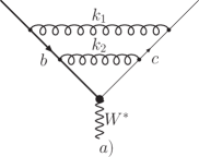
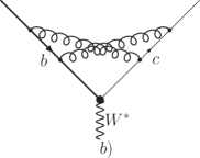
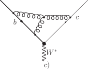
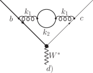
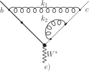
Figure 1: Sample two-loop diagrams that contribute to $b\to c+W$ transition.

Having discussed parametrization of phase-spaces that we employ in the NNLO computation, we continue with the description of technical details relevant for the computation of ${\cal O}(\alpha_{s}^{2})$ QCD corrections to $b\to cl\bar{\nu}_{l}$ transition. There are three distinct components that need to be addressed – two-loop virtual corrections, virtual corrections to single real emission process and double real emission corrections. Since these components require different techniques, we describe the relevant details in the following subsections.

2.2 Two-loop virtual corrections

We begin with the discussion of how two-loop virtual corrections are computed. There are twelve two-loop diagrams; examples are shown in Fig.1. These diagrams are complicated because they involve several mass scales, $m_{b}^{2},m_{c}^{2},W^{2},m_{l}^{2}$ as well as complicated tensor integrals, e.g. due to spin correlations of final state leptons with bottom and charm quarks. These features make analytic computations impractical. However, we can compute those diagrams numerically using the method of sector decomposition [32]. We point out that application of sector decomposition is simplified in $b$-decays, since the two-loop diagrams do not develop genuine imaginary parts. In principle, sector decomposition method was extended recently [33, 34] to deal with problems where imaginary parts do appear but it is a welcome feature of the problem at hand, that we do not need to deal with additional complications.

Hence, the primary issue in the calculation of two-loop Feynman diagrams that we have to address is the efficient choice of Feynman parameters, to reduce the amount of sectors that are created in the process of sector decomposition. It is also important to perform integration over loop momenta in such a way that computation of tensor integrals does not introduce kinematic singularities. It turns out that a very simple and fairly efficient way to deal with tensor integrals is to integrate over two loop momenta sequentially. To illustrate this procedure, we consider the planar two-loop diagram, shown in Fig.1a. This diagram can be represented as a linear combination of tensor integrals

$$I_{ij}=\int{\frac{d^{d}k_{1}}{\left(2\pi\right)^{d}}}\int{\frac{d^{d}k_{2}}{\left(2\pi\right)^{d}}}\frac{\{k_{1}\}_{i}\{k_{2}\}_{j}}{D_{1}D_{2}D_{3}D_{4}D_{5}D_{6}},\\$$ (20)

where $k_{1}$ and $k_{2}$ are the loop momenta, $\{q\}_{i}=q_{\mu_{1}}...q_{\mu_{i}}$ is the rank-$i$ tensor, composed of the relevant loop momenta and $D_{m=1..6}$ are inverse Feynman propagators that appear in the planar diagram. They read

$$D_{1}={k}^{2}_{1},\qquad D_{2}={k}^{2}_{1}+2k_{1}b,\qquad D_{3}={k}^{2}_{1}+2k_{1}c,$$ (21)

$$D_{4}={k}^{2}_{2},\qquad D_{5}=k_{12}^{2}+2k_{12}b,\qquad D_{6}=k_{12}^{2}+2k_{12}c,$$ (22)

where $k_{12}=k_{1}+k_{2}$ is used. To integrate over momentum $k_{2}$, we introduce two Feynman parameters and write

$$\int\frac{d^{d}k_{2}}{(2\pi)^{d}}\frac{\{k_{2}\}_{j}}{D_{4}D_{5}D_{6}}=2\int\limits_{0}^{1}[{\rm d}x_{2}{\rm d}x_{3}]\int\frac{d^{d}K}{(2\pi)^{d}}\frac{\{K-Q\}_{j}}{\left(K^{2}-\Delta(k_{1})\right)^{3}},$$ (23)

where $[{\rm d}x_{2}{\rm d}x_{3}]={\rm d}x_{2}{\rm d}x_{3}\theta(1-x_{2}-x_{3})$ is the integration measure and

$$K=k_{2}+Q,\;\;\;Q=\left(k_{1}+b\right)x_{2}+\left(k_{1}+c\right)x_{3},$$ (24)

$$\Delta(k_{1})=Q^{2}-\left({k}^{2}_{1}+2k_{1}b\right)x_{2}-\left({k}^{2}_{1}+2k_{1}c\right)x_{3}.$$ (25)

Integration over the shifted loop momentum $K$ is standard and can be easily performed for arbitrary rank tensor. The important point is that the higher the rank of the tensor, the smaller the power of the function $1/\Delta$ is in the resultant integral. Since numerical integration is mostly problematic because of infrared divergences, we should be looking at the most infrared-singular integral, which is provided by the $K$-less term in the numerator of Eq.(23). For such integrals we find

$$2\int\limits_{0}^{1}[{\rm d}x_{2}{\rm d}x_{3}]\int\frac{d^{d}K}{(2\pi)^{d}}\frac{\{Q\}_{j}}{\left(K^{2}-\Delta(k_{1})\right)^{3}}=-\frac{i\Gamma\left(1+\epsilon\right)}{(4\pi)^{d/2}}\int[{\rm d}x_{2}{\rm d}x_{3}]\frac{\{Q\}_{j}}{\left[\Delta(k_{1})\right]^{1+\epsilon}}.$$ (26)

Note that integrals with higher powers of $K$ in Eq.(23), can, after $K$-integration, be written as a linear combination of the integrands in the right hand side of Eq.(26), by multiplying and dividing the integrand by appropriate powers of $\Delta(k_{1})$. The important point is that additional powers of $K$ in Eq.(23) do not generate yet higher powers of $1/\Delta$ in Eq.(26).

The next step requires integration over $k_{1}$; to do that, it is convenient to change variables $x_{2}=\lambda_{1}\lambda_{2},\;x_{3}=\lambda_{1}(1-\lambda_{2})$. The integral over $k_{1}$ becomes

$$I_{ij}\to I_{i_{1}}=\int\;\frac{{\rm d}\lambda_{1}{\rm d}\lambda_{2}}{\lambda_{1}^{\epsilon}(1-\lambda_{1})^{1+\epsilon}}\int\frac{d^{d}k_{1}}{(2\pi)^{d}}\frac{\{k\}_{i_{1}}}{D_{1}D_{2}D_{3}{\tilde{\Delta}}^{1+\epsilon}},$$ (27)

where

$$\tilde{\Delta}=k_{1}^{2}+2k_{1}Q_{2}-\frac{\lambda_{1}Q_{2}^{2}}{1-\lambda_{1}},$$ (28)

and

$$Q_{2}=\lambda_{2}b+\left(1-\lambda_{2}\right)c.$$ (29)

Since $\tilde{\Delta}$ is a polynomial in $k_{1}$, the integration over $k_{1}$ can be performed in, essentially, the same way as what was described above in regard with $k_{2}$ integration. Integrals with strongest infrared divergences are the ones without additional powers of $k_{1}$ in the numerator. The corresponding scalar integral reads

$$I_{0}=\frac{\Gamma(2+2\epsilon)}{(4\pi)^{d}}\int\limits_{0}^{1}\prod\limits_{i=1}^{5}{\rm d}\lambda_{i}\frac{\lambda_{1}^{-\epsilon}(1-\lambda_{1})^{1+\epsilon}\lambda_{4}\lambda_{5}^{\epsilon}(1-\lambda_{5})^{2}}{F^{2+2\epsilon}},$$ (30)

where

$$F=(1-\lambda_{1})(Q_{3}\lambda_{4}(1-\lambda_{5})+Q_{2}\lambda_{5})^{2}+Q_{2}^{2}\lambda_{1}\lambda_{5}$$ (31)

and

$$Q_{3}=\lambda_{3}b+(1-\lambda_{3})c.$$ (32)

It is clear from Eqs.(30,31) that the function $1/F^{2+2\epsilon}$ develops overlapping singularities at the integration boundaries; for example $F=0$ for $\lambda_{1}=1,\lambda_{5}=0$ and for $\lambda_{4}=0,\lambda_{5}=0$. To disentangle those singularities, we employ the technique of sector decomposition [32]. To this end, we map all the singularities to the origin by splitting the integration region into two intervals [0,1/2] and [1/2,1], for each $\lambda_{i}$, and then change variables $\lambda_{i}\to\lambda_{i}/2$ and $\lambda_{i}\to 1-\lambda_{i}/2$ in the first and second interval, respectively. The sector decomposition is then applied to the integrand; this allows us to find a sequence of variable transformations that factorize all singularities. Once singularities are factored out, for each tensor integral we get expressions of the following type

$$I_{ij}=\sum\limits_{\alpha\in{\rm sect}}\int\limits_{0}^{1}{\rm d}\lambda_{1}{\rm d}\lambda_{2}...{\rm d}\lambda_{n}\frac{N^{\alpha}_{ij}(\lambda_{1},\lambda_{2}...\lambda_{n})}{\prod\limits_{i=1}^{n_{\alpha}}\lambda_{i}^{1+a_{i}\epsilon}D_{ij}^{\alpha}(\lambda_{1},\lambda_{2},...\lambda_{n})},$$ (33)

where all functions $N_{ij}^{\alpha}(\{\lambda_{i}\})$ and $D_{ij}^{\alpha}(\{\lambda_{i}\})$ are finite throughout the integration region. Hence, all the singularities of the integrand are in explicitly factorized form and it is easy to obtain integrable expressions by employing the plus-distribution prescription

$$\frac{1}{\lambda^{1+a\epsilon}}=\frac{-1}{a\epsilon}\delta\left(\lambda\right)+\sum_{n=0}{\left[{\frac{\ln^{n}\left(\lambda\right)}{\lambda}}\right]}_{+}\frac{(-a\epsilon)^{n}}{n!},$$ (34)

where

$$\int_{0}^{1}d\lambda f\left(\lambda\right){\left[{\frac{\ln^{n}\left(\lambda\right)}{\lambda}}\right]}_{+}=\int_{0}^{1}d\lambda\frac{f\left(\lambda\right)-f\left(0\right)}{\lambda}\ln^{n}\left(\lambda\right).$$ (35)

We are now in a position to sketch all the steps that we go through to carry out a calculation of a planar two-loop diagram. After the planar two-loop diagram is multiplied with the complex conjugate tree-level amplitude and summation over polarizations of external particle is performed, we use Form [35] to integrate over the loop momenta, following the procedure that we just described. As explained earlier, we can always write the result in a form similar to that of the scalar two-loop integral provided that we allow for a polynomial function of Feynman parameters in the numerator. Since those numerator functions are finite, we do not need to know their explicit form and can treat them as generic finite functions in the process of sector decomposition. The sector decomposition procedure is coded up in Maple [36]. After sector decomposition is completed, Fortran files that contain finite functions to be integrated and all the changes of variables that the sector decomposition procedure found necessary to apply to the integrand to factor out potential singularities, are automatically written out.

Computation of the non-planar diagram and the diagram with the three-gluon vertex is very similar to what is described above; all that changes is the Feynman parametrization. However, the procedure has to be modified for diagrams with vacuum polarization insertions on a gluon line and for diagrams with self-energy insertions on bottom and charm quark lines. We begin with the discussion of the vacuum polarization diagrams with massless particles, e.g. gluons, quarks and ghosts. Such diagrams read

$$I_{\rm VP}=\int{\frac{d^{d}k_{1}}{\left(2\pi\right)^{d}}}\int{\frac{d^{d}k_{2}}{\left(2\pi\right)^{d}}}\frac{N(k_{1},k_{2})}{{k}_{2}^{2}\left(k_{1}+k_{2}\right)^{2}\left({k}_{1}^{2}\right)^{2}\left({k}_{1}^{2}+2k_{1}b\right)\left({k}_{1}^{2}+2k_{1}c\right)}.$$ (36)

An obvious issue here is the presence of two identical gluon propagators $k_{1}^{-2}$. As the result, in the limit $k_{1}\to 0$, the denominator in Eq.(36) develops cubic, rather than linear, singularity. In principle, even in this case, it is possible to proceed along the lines described above for the planar diagram all the way through the application of the sector decomposition and factorization of singularities. However, the complication occurs in the process of the extraction of singularities using plus-distributions Eq.(34), since a term that scales like $x^{-1-n}$ for $x\to 0$, leads to an expansion that involves $n$-th derivative of a $\delta$-function rather than the $\delta$-function itself. As it turns out, this complication is unnecessary since one can analytically integrate over $k_{2}$ in any massless vacuum polarization diagram and observe that

$$\int{\frac{d^{d}k_{2}}{\left(2\pi\right)^{d}}}\frac{N(k_{1},k_{2})}{{k}_{2}^{2}\left(k_{1}+k_{2}\right)^{2}}\sim k_{1}^{2}\tilde{N}(k_{1}),$$ (37)

thanks to gauge-invariance. When dealing with massless vacuum polarization diagrams, we indeed integrate over $k_{2}$ analytically, cancel one of the $1/k_{1}^{2}$ propagators and then perform numerical integration over $k_{1}$.

Clearly, a similar problem occurs also in the case of vacuum polarization corrections with massive quarks. In that case, however, it is harder to explicitly factor out the dependence on the loop momentum $k_{1}$, to cancel the cubic divergence at small $k_{1}$. For vacuum polarizations with massive quarks we adopt a different strategy – we subtract those vacuum polarization loops at zero momentum transfer and use dispersion representation to connect the two-loop diagram with the massive fermion loop to a one-loop diagram with the massive gluon [37].

Non-integrable singularities appear also in diagrams with the self-energy insertion on the massive ($b$ or $c$) lines; in this case they are caused by the square of the massive propagator which becomes nearly on-shell for small momentum of the virtual gluon. In variance with the case of the massless vacuum polarization, it is not possible to perform analytic integration over the loop momentum of the “self-energy” loop. To get around this problem, we use a particular integral representation for the quark self-energy diagram. We consider a self-energy diagram

$$\hat{\Sigma}=\int{\frac{d^{d}k_{2}}{\left(2\pi\right)^{d}}}\frac{\gamma^{\mu}(\hat{p}+\hat{k}_{2}+m_{i})\gamma_{\mu}}{((p+k_{2})^{2}-m_{i}^{2})k_{2}^{2}},$$ (38)

where $m_{i}$ stands for $m_{b}$ or $m_{c}$. We combine two denominators using Feynman parameters, integrate over the loop momentum and obtain

$$\hat{\Sigma}=\frac{i\Gamma(\epsilon)}{(4\pi)^{d/2}}\int\limits_{0}^{1}{\rm d}xx^{-\epsilon}(p^{2}-m_{i}^{2})^{-\epsilon}\frac{\gamma^{\mu}(\hat{p}+m_{i}-\hat{p}x)\gamma_{\mu}}{(1-p^{2}x/(p^{2}-m_{i}^{2}))^{\epsilon}}.$$ (39)

This integral can be written through hypergeometric functions. To this end, we introduce two Dirac structures

$$\hat{N}_{1}=\gamma^{\mu}(\hat{p}+m_{i})\gamma_{\mu}=(2-d)\hat{p}+dm,\;\;\;\hat{N}_{2}=\gamma^{\mu}\hat{p}\gamma_{\mu}=(2-d)\hat{p},$$ (40)

and write

$$\Sigma =\frac{i\Gamma(\epsilon)}{(4\pi)^{d/2}}(p^{2}-m_{i}^{2})^{-\epsilon}\left[\hat{N}_{1}\;\;\frac{\Gamma(1-\epsilon)}{\Gamma(2-\epsilon)}F_{21}\left(\epsilon,1-\epsilon;2-\epsilon,\frac{p^{2}}{p^{2}-m_{i}^{2}}\right)\right.$$ (41)

$$\left.-\hat{N}_{2}\;\;\frac{\Gamma(2-\epsilon)}{\Gamma(3-\epsilon)}F_{21}\left(\epsilon,2-\epsilon;3-\epsilon,\frac{p^{2}}{p^{2}-m_{i}^{2}}\right)\right].$$

These hypergeometric functions are not suitable for the purpose of subsequent integration because the on-shell limit $p^{2}\to m_{i}^{2}$ is at infinity. To take care of that, it is useful to employ an identity that relates the hypergeometric functions with the argument $z$ and $z/(z-1)$. If we perform this transformation and go back to the integral representation, both of the hypergeometric functions (HGFs) become

$$(p^{2}-m_{i}^{2})^{-\epsilon}{\rm HGFs}\to\int\limits_{0}^{1}{\rm d}x\frac{x^{\epsilon-a}(1-x)^{b-2\epsilon}}{p^{2}-m_{i}^{2}/x},$$ (42)

where $a,b$ are some integers. It is now straightforward to subtract from and add to the integrand in the right hand side of Eq.(42) its value at $p^{2}=m_{i}^{2}$

$$\int\limits_{0}^{1}{\rm d}x\frac{x^{\epsilon-a}(1-x)^{b-2\epsilon}}{p^{2}-m_{i}^{2}/x}=\frac{p^{2}-m_{i}^{2}}{m_{i}^{2}}\;\int\limits_{0}^{1}{\rm d}x\frac{x^{\epsilon-a+1}(1-x)^{b-1-2\epsilon}}{p^{2}-m_{i}^{2}/x}-m_{i}^{-2}B(\epsilon-a+2,b-2\epsilon).$$ (43)

The first term in the right hand side of Eq.(43) can be inserted in a two-loop diagram since the pre-factor $p^{2}-m_{i}^{2}$ cancels one of the problematic massive fermion propagators. The second term is a constant; it can be combined with the mass counter-term contribution to cancel quadratic singularity and, after that, calculated explicitly.

2.3 Mixed real-virtual corrections

In this subsection we discuss the calculation of one-loop radiative corrections to single gluon real emission amplitudes. At first sight, these corrections may look much simpler than the two-loop virtual corrections discussed previously, since they involve only one-loop virtual diagrams and the final state with relatively low multiplicity. It would appear therefore that, technically, they fall into a category of well-established next-to-leading (NLO) calculations [38]. Unfortunately, this is not quite true since, in contrast to standard NLO computations, the emitted gluon in the final state can become soft, invalidating applicability of NLO computational techniques. Therefore, real-virtual corrections require careful study.

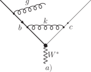
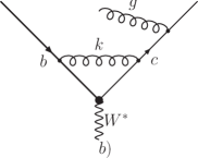
Figure 2: Sample diagrams that describe one-loop corrections to $b\to c+W+g$ transition.

There are two strategies that one can pursue to deal with the real-virtual corrections. One can use Passarino-Veltman tensor reduction technique [38] and integration-by-parts identities [39] to reduce real-virtual corrections to one-loop scalar integrals. Then, one can attempt to extract singularities that appear when the energy of the gluon in the final state becomes small. While this approach was used in a number of calculations [24, 25], it rapidly becomes impractical with the increase in the number of particles in the final state.

A flexible method should be based on numerical computations and it seems that Feynman parametrization of one-loop virtual corrections and subsequent application of sector decomposition to both Feynman parameters and the energy of the emitted gluon is a straightforward thing to do. The only problem with that approach is that one-loop corrections to real gluon emission do develop imaginary parts, even when all parameters in the integrand are real. Technically this happens because of the singularity on the real integration axis which is regulated by the $+i0$ prescription. While it is easy to implement such a prescription in analytical computations, it is difficult to do so in a fully numerical approach.

It turns out that there is a simple way to avoid the issue of the imaginary part in this problem. To this end, we observe that, for any Feynman diagram of the real-virtual type that contributes to $b\to c$ transition, it is possible to choose integration variables in such a way that the integration over at least one variable is of the form

$$I=\int{\rm d}{\mbox{\boldmath$x$}}\int\limits_{0}^{1}{\rm d}yF({\mbox{\boldmath$x$}},y),\;\;\;F({\mbox{\boldmath$x$}},y)=\frac{y^{n_{1}-n_{2}\epsilon}}{\left(-A(\{{\bf x}\})+B(\{{\bf x}\})y+i0\right)^{n_{3}+n_{4}\epsilon}}.$$ (44)

In Eq.(44) $x$ is a collection of other variables involved in the computation of the integral, $A$ and $B$ are some functions of those variables which satisfy $B(\{{\mbox{\boldmath$x$}}\})>A(\{{\mbox{\boldmath$x$}}\})$ for all $x$ and $n_{i=1..4}$ are integers. We do not have a proof that such a parametrization is possible for real-virtual corrections under all possible circumstances, but we find empirically that it exists for $b\to c$ transitions.

The problem with the numerical evaluation of the integral in Eq.(44) is that, for $n_{3}>0$, it becomes singular at $y=A({\mbox{\boldmath$x$}})/B({\mbox{\boldmath$x$}})<1$, so that this singularity occurs in the middle of the integration region. Such singularity can not be included into the sector decomposition framework in a straightforward way. To deal with this problem, we rewrite Eq.(44) in the following manner

$$I=\int{\rm d}{\mbox{\boldmath$x$}}\int\limits_{0}^{\infty}{\rm d}y\;F({\mbox{\boldmath$x$}},y)-\int{\rm d}{\mbox{\boldmath$x$}}\int\limits_{1}^{\infty}{\rm d}y\;F({\mbox{\boldmath$x$}},y),$$ (45)

and observe that the first integral can be computed analytically, while denominator of the function $F(x,y)$ in the second term is sign-definite. Changing variables $y\to 1/y$ in the second term in Eq.(45), we obtain the integral that is amenable to sector decomposition.

We now illustrate this general discussion by considering explicit examples. To set the stage, we begin with a simple case, where the imaginary part problem does not occur. This happens for all diagrams where the gluon is emitted from the $b$-quark line. For our example, we consider diagram Fig. 2a. Interference of this diagram with the tree amplitude that describes radiative decay of the $b$-quark $b\to c+W+g$, contributes to ${\cal O}(\alpha_{s}^{2})$ correction to the decay rate. We consider a scalar integral associated with this loop diagram

$$I=\frac{1}{\Gamma(1+\epsilon)}\int\frac{d^{d}k}{i\pi^{d/2}}\frac{1}{k^{2}\left(k^{2}+2k\left(b-g\right)-2bg\right)\left(k^{2}+2kc\right)}.$$ (46)

We introduce Feynman parameters and integrate over the loop momentum to obtain

$$I=\int\frac{[{\rm d}x_{2}{\rm d}x_{3}]}{\left[\left(\left(b-g\right)x_{2}+cx_{3}\right)^{2}+2bgx_{2}\right]^{1+\epsilon}}=\int\limits_{0}^{1}{\rm d}\lambda_{1}{\rm d}\lambda_{2}\frac{\lambda_{1}^{-\epsilon}}{\left[\Delta(\lambda_{1},\lambda_{2})\right]^{1+\epsilon}},$$ (47)

where

$$\Delta(\lambda_{1},\lambda_{2})=\lambda_{1}\left(\left(b-g\right)\lambda_{2}+c(1-\lambda_{2})\right)^{2}+2bg\lambda_{2}.$$ (48)

Writing $b-g=c+W$, we find

$$\Delta=\lambda_{1}(m_{c}^{2}+2cW\lambda_{2}+W^{2}\lambda_{2}^{2})+2bg\lambda_{2}>0,$$ (49)

for all values $0<\lambda_{1},\lambda_{2}<1$. This representation for $\Delta(\lambda_{1},\lambda_{2})$ is instructive since it shows how new overlapping singularities appear when the emitted gluon becomes soft. Indeed, for non-vanishing gluon energy, $\Delta(\lambda_{1},\lambda_{2})$ vanishes for $\lambda_{1}=\lambda_{2}=0$. On the other hand, if the gluon is soft $g\to 0$, $\Delta(\lambda_{1},\lambda_{2})$ vanishes for $\lambda_{1}=0$ and any value of $\lambda_{2}$. To take care of all possible cases, we employ explicit parametrization of the gluon energy in the $b$-quark rest frame, as described in the previous Section, and perform sector decomposition of the amplitude squared treating $\lambda_{1},\lambda_{2}$ and $bg$ on equal footing. This allows us to extract all singularities associated with vanishing of both, the loop momentum and the momentum of the gluon in the final state.

We now turn to the description of a more difficult case which occurs when, in the one-loop amplitude, the gluon is emitted from the charm quark line. A representative diagram is shown in Fig.2. All the problems that appear in this case can be illustrated by considering the scalar integral as an example. We have

$$I=\frac{1}{\Gamma(1+\epsilon)}\int\frac{d^{d}k}{i\pi^{d/2}}\frac{1}{k^{2}\left(k^{2}+2kb\right)\left((k+c+g)^{2}-m_{c}^{2}\right)}$$

$$=\int\frac{[{\rm d}x_{2}{\rm d}x_{3}]}{\left[\left(bx_{2}+\left(g+c\right)x_{3}\right)^{2}-2gcx_{3}\right]^{1+\epsilon}}.$$ (50)

Changing variables $x_{2}=\lambda_{1}(1-\lambda_{2})$ and $x_{3}=\lambda_{1}\lambda_{2}$, we obtain

$$I=\int{\rm d}\lambda_{1}{\rm d}\lambda_{2}\frac{{\lambda}_{1}^{-\epsilon}}{\left(\Delta\lambda_{1}-2cg\lambda_{2}\right)^{1+\epsilon}}=\int{\rm d}\lambda_{1}{\rm d}\lambda_{2}\frac{{\lambda}_{1}^{-\epsilon}}{\Delta^{1+\epsilon}\left(\lambda_{1}-\xi\right)^{1+\epsilon}},$$ (51)

where

$$\Delta=(b-W\lambda_{2})^{2},\;\;\;\xi=\frac{2cg\lambda_{2}}{\Delta}<1.$$ (52)

It is clear from Eq.(51) that there is a singularity at $\lambda_{1}=\xi$, i.e. in the middle of the integration region, which can not be dealt with using the sector decomposition. To transform Eq.(51) into a form suitable for numerical integration, we proceed along the lines described in the beginning of this Section. Consider integration over $\lambda_{1}$. Allowing for a general form of the integrand, we re-write

$$\int\limits_{0}^{1}{\rm d}\lambda_{1}\frac{\lambda_{1}^{a-\epsilon}}{(\lambda_{1}-\xi)^{b+\epsilon}}=\int\limits_{0}^{\infty}{\rm d}\lambda_{1}\frac{\lambda_{1}^{a-\epsilon}}{(\lambda_{1}-\xi)^{b+\epsilon}}-\int\limits_{1}^{\infty}{\rm d}\lambda_{1}\frac{\lambda_{1}^{a-\epsilon}}{(\lambda_{1}-\xi)^{b+\epsilon}}$$

$$=\xi^{1+a-b-2\epsilon}\Gamma(1-b-\epsilon)\left((-1)^{b+\epsilon}\frac{\Gamma(a+1-\epsilon)}{\Gamma(2+a-b-2\epsilon)}+\frac{\Gamma(2\epsilon-a+b-1)}{\Gamma(\epsilon-a)}\right)$$

$$-\int\limits_{0}^{1}{\rm d}\lambda_{1}\frac{\lambda_{1}^{b-a+2\epsilon-2}}{(1-\xi\lambda_{1})^{b+\epsilon}}.$$ (53)

The remaining integrand is sign-definite, because $\xi<1$. The problem of the singularity in the middle of the integration region has been handled by an analytic integration; the remnant of this problem is the imaginary part in $(-1)^{b+\epsilon}$. It is now very straightforward to apply the sector decomposition to the remaining integral in Eq.(53), to extract the infrared singularities.

The above technique is applicable to all real-virtual diagrams. The first step – finding Feynman parametrization that is linear in (at least) one variable – requires careful inspection of each diagram individually but, once such parametrization is found, remaining steps are easily accomplished using algebraic manipulation programs. A slightly different approach is required for real-virtual contributions related to self-energy insertions on massive fermion lines where quadratic singularities appear. We deal with those singularities using parametrization of self-energy diagrams described earlier in this Section in the context of two-loop virtual corrections.

2.4 Double real emission corrections

Finally, we address the computation of the double real emission corrections. Because we deal primarily with massive quarks, the majority of diagrams develop only infrared singularities. We can easily extract those using explicit parametrization of gluon energies in the $b$-quark rest frame, discussed earlier in this Section. The only exception to the “no collinear singularity” rule comes from diagrams where an off-shell gluon splits into two gluons or a $q\bar{q}$ pair. In principle, since we use the relative angle between two gluons (or massless quarks) as one of the primary variables for the phase-space parametrization, extraction of (potential) collinear singularity is also straightforward. However, the complication arises because of the necessity to deal with the extraction of quadratic singularities in some of the diagrams. The problem and the solution is best illustrated by considering diagrams with a massless $q\bar{q}$ pair in the final state.

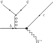
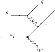
Figure 3: Diagrams that describe double real emission process with a massless $q\bar{q}$ pair in the final state.

Consider two diagrams that contribute to the process $b\to cl\bar{\nu}_{l}+q\bar{q}$, shown in Fig.3. Upon squaring these diagrams, we find that the gluon splitting $g^{*}\to q\bar{q}$ leads to a structure that involves square of the gluon propagator

$$\frac{q_{\mu}{\bar{q}}_{\nu}+q_{\nu}{\bar{q}}_{\mu}-g_{\mu\nu}q{\bar{q}}}{(q\bar{q})^{2}}.$$ (54)

An obvious problem with this result is that the singularity associated with the collinear limit is power-like; hence, we can not disregard the numerator in the process of the sector-decomposition since it provides the necessary $q\bar{q}$ scalar product to soften the collinear singularity. The question is how to parametrize the momenta $q,\bar{q}$ to enable easy extraction of the scalar product $q\bar{q}$ from the numerator in Eq.(54). To deal with this problem, we need to exploit the fact that, when collinear singularity occurs in those diagrams, the momenta of $q$ and $\bar{q}$ become parallel to each other. We use this feature to parametrize the scalar products of $q$ and $\bar{q}$ momenta with, say, the charm quark momentum in the following way

$$c\bar{q}=\frac{b\bar{q}}{bq}cq+\sqrt{x_{4}}x_{1}x_{2}\Delta_{c\bar{q}}.$$ (55)

Here $x_{4}$ describes the angle between $q$ and $\bar{q}$, $\cos\theta_{12}=1-2x_{4}$. The important point is the factor $\sqrt{x_{4}}$ in the second term on the right hand side in Eq.(55); it is crucial for regulating collinear singularity. On the other hand, the (complicated) function $\Delta_{c\bar{q}}$ does not need to be made explicit in the matrix element to cancel collinear singularity. Nevertheless, we give it here for completeness

$$\Delta_{c\bar{q}}=\frac{4p_{c}\left((m_{b}-m_{c})^{2}-m_{l}^{2}\right)(1-x_{3})\left(\sqrt{x_{4}}\cos\theta_{1c}-\sqrt{1-x_{4}}\sin\theta_{1c}\cos\phi_{c}\right)}{2(m_{b}-E_{c}+p_{c}\cos\theta_{2c})-E_{g_{1}}(1-\cos\theta_{12})}.$$ (56)

Very similar manipulations are needed for scalar products that involve the momentum of the charged lepton and the momenta of $q$ and $\bar{q}$.

3 Results

In this Section, we discuss the two-loop QCD radiative corrections to $b\to X_{c}l\bar{\nu}_{l}$ transitions and present results for a large number of moments, relevant for the experimental analysis and semileptonic fits. We begin by writing the decay rate $b\to X_{c}l\bar{\nu}_{l}$ as

$$d\Gamma=\frac{G_{F}^{2}\left|V_{cb}\right|^{2}m^{5}_{b}}{192{\pi}^{3}}\left(dF_{0}+\frac{\alpha_{s}}{\pi}dF_{1}+\left(\frac{\alpha_{s}}{\pi}\right)^{2}dF_{2}+{\cal O}(\alpha_{s}^{3})\right),$$ (57)

where ${\rm d}F_{i}$ stands for the differential decay rate, at leading, next-to-leading and next-to-next-to-leading order, respectively. The strong coupling constant $\alpha_{s}=\alpha_{s}(m_{b})$ is defined in the ${\overline{\rm MS}}$ scheme in the theory with three massless flavors; it is renormalized at the value of the $b$-quark mass. The lepton and hadron moments are defined as

$$L_{n}\left(E_{\rm cut}\right)=\frac{\langle{\left(E_{l}/m_{b}\right)}^{n}\theta\left(E_{l}-E_{\rm cut}\right)d\Gamma\rangle}{\langle d\Gamma_{0}\rangle},$$ (58)

$$H_{ij}\left(E_{\rm cut}\right)=\frac{\langle\left(({m}_{h}^{2}-{m}_{c}^{2})/m_{b}^{2}\right)^{i}\left(E_{h}/m_{b}\right)^{j}\theta\left(E_{l}-E_{\rm cut}\right)d\Gamma\rangle}{\langle d\Gamma_{0}\rangle},$$ (59)

where $E_{l,h}$ are the lepton and hadron energies in the $b$-quark rest frame and $m_{h}$ is hadronic invariant mass. Also,

$$d\Gamma_{0}=\frac{G_{F}^{2}\left|V_{cb}\right|^{2}m^{5}_{b}}{192{\pi}^{3}}dF_{0},$$ (60)

and $\langle..\rangle$ implies integration of the corresponding quantity over available phase-space. The calculation is performed in the pole mass scheme. For numerical integration, we use Vegas [40], implemented in the Cuba library [41]. We treat the axial current as suggested in Ref.[42].

The lepton and hadron moments can be computed in an expansion in the strong coupling constant

$$L_{n}={L}^{\left(0\right)}_{n}+\frac{\alpha_{s}}{\pi}L^{\left(1\right)}_{n}+\left(\frac{\alpha_{s}}{\pi}\right)^{2}\left(\beta_{0}L^{\left(2,BLM\right)}_{n}+L^{\left(2\right)}_{n}\right)+...,$$ (61)

$$H_{ij}={H}^{\left(0\right)}_{ij}+\frac{\alpha_{s}}{\pi}H^{\left(1\right)}_{ij}+\left(\frac{\alpha_{s}}{\pi}\right)^{2}\left(\beta_{0}H^{\left(2,BLM\right)}_{ij}+H^{\left(2\right)}_{ij}\right)+...,$$ (62)

where $\beta_{0}=11-2/3n_{f}$, and $n_{f}=3$ is the number of quark flavors that are treated as massless in the computation. Next-to-leading order and BLM corrections [43] to any kinematic distribution in $b\to X_{c}l\bar{\nu}_{l}$ transition are known [15, 16, 17, 18, 19]. Non-BLM corrections $L_{n}^{(2)},H_{ij}^{(2)}$ for massless lepton were computed very recently and their detailed investigation is not available. In the remainder of this Section, we study non-BLM corrections to $b\to X_{c}e\bar{\nu}_{e}$ decay in detail. Then we describe results for the inclusive rate $b\to X_{c}\tau\bar{\nu}_{\tau}$.

	$r$ \$\xi$	0.0	0.1	0.2	0.3	0.4	0.5	0.6	0.7
${L}_{0}^{(2)}$	0.2	4.01(6)	3.98(6)	3.93(7)	3.73(9)	3.3(1)	3.1(1)	2.47(9)	2.08(8)
${L}_{0}^{(2)}$	0.22	3.74(5)	3.72(6)	3.62(7)	3.48(8)	3.19(9)	2.79(9)	2.34(9)	1.87(7)
${L}_{0}^{(2)}$	0.24	3.50(5)	3.50(5)	3.35(6)	3.24(7)	2.88(8)	2.57(9)	2.28(7),	1.66(6)
${L}_{0}^{(2)}$	0.25	3.38(4)	3.37(5)	3.30(6)	3.14(7)	2.84(8)	2.61(8)	2.14(7)	1.54(5)
${L}_{0}^{(2)}$	0.26	3.27(4)	3.26(4)	3.14(5)	3.03(7)	2.78(7)	2.44(7)	1.95(6)	1.49(5)
${L}_{0}^{(2)}$	0.28	3.05(4)	3.02(4)	2.95(5)	2.84(6)	2.56(6)	2.32(7)	1.80(6)	1.29(4)
${L}_{1}^{(2)}$	0.2	1.38(2)	1.38(2)	1.36(2)	1.35(2)	1.30(3)	1.15(3)	1.04(3)	0.90(3)
${L}_{1}^{(2)}$	0.22	1.26(1)	1.26(1)	1.25(2)	1.23(2)	1.16(2)	1.12(2)	0.93(3)	0.82(3)
${L}_{1}^{(2)}$	0.24	1.16(1)	1.16(1)	1.15(1)	1.14(2)	1.05(2)	1.00(3)	0.87(2)	0.71(2)
${L}_{1}^{(2)}$	0.25	1.11(1)	1.11(1)	1.09(1)	1.07(2)	1.01(2)	0.93(2)	0.86(2)	0.65(2)
${L}_{1}^{(2)}$	0.26	1.06(1)	1.06(1)	1.06(1)	1.03(2)	0.99(2)	0.90(2)	0.75(2)	0.61(2)
${L}_{1}^{(2)}$	0.28	0.97(1)	0.97(1)	0.96(1)	0.94(1)	0.89(2)	0.83(2)	0.70(2)	0.53(1)
${L}_{2}^{(2)}$	0.2	0.514(6)	0.514(6)	0.513(6)	0.508(6)	0.501(7)	0.466(9)	0.45(1)	0.38(1)
${L}_{2}^{(2)}$	0.22	0.464(5)	0.464(5)	0.462(5)	0.462(6)	0.454(7)	0.422(9)	0.410(9)	0.333(9)
${L}_{2}^{(2)}$	0.24	0.417(4)	0.417(4)	0.416(5)	0.413(5)	0.402(6)	0.377(7)	0.339(8)	0.300(7)
${L}_{2}^{(2)}$	0.25	0.395(4)	0.395(4)	0.395(4)	0.392(5)	0.376(6)	0.367(7)	0.336(7)	0.275(7)
${L}_{2}^{(2)}$	0.26	0.375(4)	0.375(4)	0.374(4)	0.372(4)	0.361(5)	0.345(6)	0.306(7)	0.248(6)
${L}_{2}^{(2)}$	0.28	0.336(3)	0.336(3)	0.336(4)	0.331(5)	0.324(6)	0.290(6)	0.274(6)	0.215(6)
${L}_{3}^{(2)}$	0.2	0.202(2)	0.202(2)	0.202(2)	0.201(2)	0.197(3)	0.194(3)	0.182(4)	0.159(4)
${L}_{3}^{(2)}$	0.22	0.179(2)	0.179(2)	0.179(2)	0.178(2)	0.177(2)	0.172(3)	0.163(3)	0.139(3)
${L}_{3}^{(2)}$	0.24	0.158(1)	0.158(2)	0.158(1)	0.158(1)	0.157(2)	0.151(2)	0.141(3)	0.120(3)
${L}_{3}^{(2)}$	0.25	0.149(1)	0.149(1)	0.149(1)	0.148(1)	0.147(2)	0.142(2)	0.127(3)	0.114(2)
${L}_{3}^{(2)}$	0.26	0.140(1)	0.140(1)	0.139(1)	0.139(1)	0.138(2)	0.132(2)	0.121(2)	0.106(3)
${L}_{3}^{(2)}$	0.28	0.123(1)	0.123(1)	0.123(1)	0.122(1)	0.120(1)	0.117(2)	0.107(2)	0.085(2)

Table 1: Non-BLM corrections to lepton moments $L_{i}^{\left(2\right)}$ in dependence of $r$ and $\xi$. Vegas integration errors are shown in brackets.

3.1 Non-BLM corrections and moments of $b\to X_{c}e\bar{\nu}_{e}$ decays

In this subsection, we study corrections to semileptonic decay $b\to X_{c}l\bar{\nu}_{l}$, where $l$ is the massless lepton, in dependence of the bottom and charm quark masses, and the lepton energy cut. Because lepton and hadron moments defined in Eq.(61) and Eq.(62) are dimensionless, they depend on the two ratios of the three dimensionfull parameters. We choose $r=m_{c}/m_{b}$ and $\xi=2E_{\rm cut}/m_{b}$ as independent variables. In Table 1 we show non-BLM corrections to lepton moments $L_{0,1,2,3}$ for a number of $r$ and $\xi$ values. In Tables 2,3 results for hadron moments are given. These results can, in principle, be used in global fits of semileptonic decays where $b$ and $c$ masses are parameters that need to be fitted.

It was observed in [23] that second order QCD corrections to $b$-decays do not depend strongly on kinematics and it is interesting to further explore this observation. To this end, we may conjecture that non-BLM corrections to moments are given by constant, $\xi$-independent renormalization factors of the leading order moments. If true, this renormalization factor can be determined from Refs. [26, 27], where lepton and hadron energy moments are analytically computed for zero lepton energy cut. We will construct the interpolating function for lepton energy moments, following this observation. At leading order, the lepton energy moments are given by

$${L}_{i}^{(0)}(r,\xi)=\frac{Y_{i}(r,\xi)}{Y_{0}(r,0)},$$ (63)

where

$$Y_{i}(r,\xi)=\int_{\xi}^{x_{m}}{\rm d}x\left[\frac{2x^{2}\left(x_{m}-x\right)^{2}}{\left(1-x\right)^{3}}\right]\\ \left(6-6x+xx_{m}+2x^{2}-3x_{m}\right)\left(\frac{x}{2}\right)^{i}.$$ (64)

In Eq.(64) $x_{m}=1-r^{2}$ and the integration is over $x=2E_{l}/m_{b}$. Since the integration here is elementary but the resulting formulas are lengthy, we do not present the results of the integration here. We introduce the interpolating function by defining

$$L_{i}^{(2),\rm in}(r,\xi)=\frac{L_{i}^{(2)}(r,0)}{L_{i}^{(0)}(r,0)}L_{i}^{(0)}(r,\xi),$$ (65)

so that the normalization of the non-BLM correction to the moment is fixed by its value at zero lepton energy cut and the shape is taken to coincide with the leading order shape. The interpolated moments $L_{i}^{(2),\rm in}(r,\xi)$ are given in Table 4. Comparing computed and interpolated moments, we observe that $L_{i}^{(2),\rm in}(r,\xi)$ provides excellent approximation to $L_{i}^{(2)}(r,\xi)$ for small values of $\xi$. However, the agreement becomes progressively worse for larger values of $\xi$. For example, a typical deviation between the interpolated and the explicitly computed non-BLM moments for $\xi=0.7$ and $m_{c}/m_{b}=0.28$ can be as much as twenty percent. Finally, we point out that a very similar behavior is observed for non-BLM hadron energy moments.

	$r$ \$\xi$	0.0	0.1	0.2	0.3	0.4	0.5	0.6	0.7
${H}_{01}^{(2)}$	0.2	1.39(3)	1.38(3)	1.32(4)	1.28(5)	1.19(5)	1.19(5)	0.94(4)	0.78(3)
${H}_{01}^{(2)}$	0.22	1.34(3)	1.33(3)	1.32(3)	1.24(4)	1.16(4)	1.08(4)	0.85(4)	0.72(3)
${H}_{01}^{(2)}$	0.24	1.29(2)	1.28(3)	1.23(3)	1.15(3)	1.09(4)	1.02(4)	0.88(3)	0.65(3)
${H}_{01}^{(2)}$	0.25	1.27(2)	1.26(2)	1.21(3)	1.18(3)	1.05(3)	0.95(4)	0.76(3)	0.64(2)
${H}_{01}^{(2)}$	0.26	1.24(2)	1.23(2)	1.18(3)	1.11(3)	1.00(3)	0.95(3)	0.76(3)	0.60(2)
${H}_{01}^{(2)}$	0.28	1.20(2)	1.19(2)	1.15(3)	1.12(3)	0.99(3)	0.89(3)	0.69(2)	0.54(2)
${H}_{02}^{(2)}$	0.2	0.46(1)	0.46(1)	0.47(2)	0.42(2)	0.38(2)	0.39(2)	0.35(2)	0.28(1)
${H}_{02}^{(2)}$	0.22	0.46(1)	0.46(1)	0.44(2)	0.45(2)	0.39(2)	0.39(2)	0.31(2)	0.27(1)
${H}_{02}^{(2)}$	0.24	0.46(1)	0.46(1)	0.45(1)	0.44(2)	0.38(2)	0.35(2)	0.33(1)	0.26(1)
${H}_{02}^{(2)}$	0.25	0.46(1)	0.46(1)	0.45(1)	0.45(2)	0.41(2)	0.35(2)	0.34(1)	0.25(1)
${H}_{02}^{(2)}$	0.26	0.46(1)	0.45(1)	0.44(1)	0.42(2)	0.38(2)	0.37(2)	0.32(1)	0.24(1)
${H}_{02}^{(2)}$	0.28	0.46(1)	0.46(1)	0.45(1)	0.44(2)	0.39(2)	0.33(1)	0.30(1)	0.24(1)
${H}_{03}^{(2)}$	0.2	0.140(7)	0.137(8)	0.140(9)	0.12(1)	0.14(1)	0.14(1)	0.122(8)	0.104(6)
${H}_{03}^{(2)}$	0.22	0.146(6)	0.143(7)	0.142(8)	0.152(9)	0.13(1)	0.125(9)	0.123(7)	0.107(5)
${H}_{03}^{(2)}$	0.24	0.152(6)	0.150(6)	0.143(7)	0.145(9)	0.124(9)	0.132(8)	0.133(8)	0.095(5)
${H}_{03}^{(2)}$	0.25	0.155(5)	0.153(6)	0.158(7)	0.145(8)	0.150(8)	0.133(8)	0.124(7)	0.103(4)
${H}_{03}^{(2)}$	0.26	0.158(5)	0.157(6)	0.155(7)	0.152(8)	0.140(9)	0.145(7)	0.130(6)	0.101(4)
${H}_{03}^{(2)}$	0.28	0.164(5)	0.162(6)	0.158(7)	0.164(8)	0.153(7)	0.128(7)	0.125(6)	0.096(4)

Table 2: Non-BLM corrections to hadron energy moments $H_{0i}^{(2)}$ in dependence of $r$ and $\xi$. Vegas integration errors are shown in brackets.

Note that by increasing the cut on the lepton energy, the phase-space is restricted to the region where soft gluon radiation becomes relatively more important and, hence, the dynamics of the final state changes with the increase of the cut on the lepton energy. It is therefore clear that for moments defined in Eqs.(61,62) perturbative corrections at different lepton energy cuts are not correlated, i.e. different physics becomes important for different values of the lepton energy cut. On the other hand, we point out that the moments measured in experimental analysis correspond to ratios of $L$-moments defined in Eqs.(61,62); as we explain below, this difference is essential for understanding importance of QCD radiative corrections in the global fits.

We turn to the discussion of the potential impact that computed corrections may have on the extraction of fundamental quantities in heavy quark physics, such as $|V_{cb}|,m_{b},m_{c},\mu_{\pi}^{2},\,\mu_{G}^{2}$ etc. from global fits to semileptonic moments. We stress that we do not attempt to perform a fit to data on semileptonic moments, leaving this task to experts. However, we find it instructive to illustrate shifts that may be expected in the values of, e.g. the $|V_{cb}|$ and the $b$-quark mass, if non-BLM corrections are included.

	$r$ \$\xi$	0.0	0.1	0.2	0.3	0.4	0.5	0.6	0.7
${H}_{10}^{(2)}$	0.2	-0.443	-0.441	-0.423	-0.387	-0.331	-0.259	-0.181	-0.107(1)
${H}_{10}^{(2)}$	0.22	-0.402	-0.399	-0.383	-0.347	-0.294	-0.228	-0.156	-0.090(1)
${H}_{10}^{(2)}$	0.24	-0.364	-0.361	-0.346	-0.313	-0.262	-0.200	-0.134	-0.0739
${H}_{10}^{(2)}$	0.25	-0.346	-0.343	-0.328	-0.296	-0.246	-0.187	-0.124	-0.0662
${H}_{10}^{(2)}$	0.26	-0.329	-0.326	-0.311	-0.280	-0.231	-0.174	-0.114	-0.0602
${H}_{10}^{(2)}$	0.28	-0.297	-0.295	-0.280	-0.250	-0.205	-0.151	-0.0966	-0.0484(4)
${H}_{11}^{(2)}$	0.2	-0.215	-0.213	-0.204	-0.184	-0.155	-0.120(1)	-0.082(1)	-0.0479(4)
${H}_{11}^{(2)}$	0.22	-0.198	-0.197	-0.188	-0.169	-0.141	-0.107(1)	-0.0721	-0.0408(3)
${H}_{11}^{(2)}$	0.24	-0.183	-0.181	-0.173	-0.154	-0.128	-0.0956	-0.0632	-0.0342(3)
${H}_{11}^{(2)}$	0.25	-0.175	-0.174	-0.165	-0.147	-0.121(1)	-0.0900	-0.0590	-0.0313
${H}_{11}^{(2)}$	0.26	-0.168	-0.167	-0.158	-0.141	-0.114(1)	-0.0848	-0.0548	-0.0284
${H}_{11}^{(2)}$	0.28	-0.155	-0.153	-0.145	-0.128	-0.103(1)	-0.0748	-0.0469	-0.0232(2)
${H}_{12}^{(2)}$	0.2	-0.107	-0.106	-0.100	-0.090	-0.0747	-0.0565	-0.0383	-0.0217
${H}_{12}^{(2)}$	0.22	-0.0998	-0.0989	-0.0937	-0.0837	-0.0688	-0.0513	-0.0341	-0.0189
${H}_{12}^{(2)}$	0.24	-0.0935	-0.0926	-0.0877	-0.0773	-0.0629	-0.0468	-0.0304	-0.0161
${H}_{12}^{(2)}$	0.25	-0.0905	-0.0896	-0.0846	-0.0748	-0.0604	-0.0443	-0.0285	-0.0148
${H}_{12}^{(2)}$	0.26	-0.0876	-0.0867	-0.0817	-0.0719	-0.0579	-0.0423	-0.0267	-0.0136
${H}_{12}^{(2)}$	0.28	-0.0820	-0.0810	-0.0761	-0.0664	-0.0531	-0.0377	-0.0234	-0.0113

Table 3: Non-BLM corrections to hadron invariant mass moments ${H}_{1j}^{(2)}$ in dependence of $r$ and $\xi$. Vegas integration errors are shown in brackets. Integration errors are not shown if they are significantly smaller than one percent.

We begin with the discussion of the CKM matrix element $|V_{cb}|$. Since the $|V_{cb}|$ is obtained from the normalization of the partial decay rate, it is mostly sensitive to QCD corrections to the moment $L_{0}$. The non-BLM corrections to that moment for $\xi=0$ and various values of $r$ are shown in Fig.4. We see that, for realistic ratios of quark masses, the non-BLM corrections to $L_{0}$ are between $2$ and $1.5$ percent. Since experimental measurement fixes $|V_{cb}|^{2}L_{0}$, one can expect that $|V_{cb}|$ changes by about $-1$ percent, when non-BLM corrections are included. This is compatible with the uncertainty in $|V_{cb}|$ as currently estimated.

Figure 4: Non-BLM correction to the total rate, in percent, for zero lepton energy cut, as a function of the charm quark mass to bottom quark mass ratio. We use $\alpha_{s}=0.22$.

BABAR collaboration measured a number of lepton energy moments for $b\to cl\bar{\nu}_{l}$ transitions with high precision [6]. For the illustration, we use their measurement of the moment ${\cal M}_{1}$ for two values of the lepton energy cut

$${\cal M}_{1}(E_{\rm cut})=\frac{\int\limits_{E_{\rm cut}}E_{l}\;{\rm d}\Gamma}{\int\limits_{E_{\rm cut}}{\rm d}\Gamma}\;\;=\left\{\begin{array}[]{cc}1437.6(4.0)(5.7)~{}{\rm MeV},&E_{\rm cut}=0.6~{}{\rm GeV};\\ 1773.7(1.9)(1.1)~{}{\rm MeV},&E_{\rm cut}=1.5~{}{\rm GeV}.\end{array}\right.$$ (66)

These (and other) results are used to extract the following values of the bottom and charm quark masses in the kinetic scheme [44] $m_{b}^{\rm fit}=4.55(5)~{}{\rm GeV}$ and $m_{c}^{\rm fit}=1.08(7)~{}{\rm GeV}$, where we combined all uncertainties in quadratures. In terms of lepton moments computed in this paper, and neglecting non-perturbative contributions, we find

$${\cal M}_{1}(E_{\rm cut})=m_{b}{\cal M}_{1}^{\rm pt},\;\;\;\;\;{\cal M}_{1}^{\rm pt}=\frac{L_{1}(E_{l\rm cut})}{L_{0}(E_{\rm cut})}.$$ (67)

	$r$ \$\xi$	0	0.1	0.2	0.3	0.4	0.5	0.6	0.7
${L}_{0}^{(2)\rm in}$	0.2	4.01	4.00	3.94	3.77	3.48	3.05	2.48	1.77
${L}_{0}^{(2)\rm in}$	0.22	3.74	3.74	3.68	3.51	3.23	2.80	2.25	1.57
${L}_{0}^{(2)\rm in}$	0.24	3.50	3.49	3.43	3.27	2.99	2.58	2.04	1.38
${L}_{0}^{(2)\rm in}$	0.25	3.38	3.37	3.30	3.15	2.88	2.47	1.93	1.29
${L}_{0}^{(2)\rm in}$	0.26	3.27	3.26	3.19	3.05	2.77	2.36	1.83	1.20
${L}_{0}^{(2)\rm in}$	0.28	3.05	3.04	2.97	2.83	2.56	2.16	1.64	1.03
${L}_{1}^{(2)\rm in}$	0.2	1.38	1.36	1.36	1.33	1.28	1.18	1.01	0.77
${L}_{1}^{(2)\rm in}$	0.22	1.26	1.26	1.25	1.23	1.18	1.08	0.91	0.68
${L}_{1}^{(2)\rm in}$	0.24	1.16	1.16	1.15	1.13	1.08	0.98	0.82	0.59
${L}_{1}^{(2)\rm in}$	0.25	1.11	1.11	1.10	1.08	1.03	0.93	0.77	0.55
${L}_{1}^{(2)\rm in}$	0.26	1.06	1.06	1.05	1.03	0.98	0.88	0.73	0.51
${L}_{1}^{(2)\rm in}$	0.28	0.97	0.97	0.96	0.94	0.89	0.80	0.65	0.43
${L}_{2}^{(2)\rm in}$	0.2	0.514	0.514	0.514	0.510	0.500	0.475	0.425	0.339
${L}_{2}^{(2)\rm in}$	0.22	0.464	0.464	0.464	0.461	0.450	0.426	0.377	0.295
${L}_{2}^{(2)\rm in}$	0.24	0.417	0.417	0.417	0.414	0.404	0.380	0.332	0.253
${L}_{2}^{(2)\rm in}$	0.25	0.395	0.395	0.395	0.392	0.382	0.358	0.312	0.234
${L}_{2}^{(2)\rm in}$	0.26	0.375	0.375	0.375	0.372	0.362	0.338	0.292	0.216
${L}_{2}^{(2)\rm in}$	0.28	0.336	0.336	0.336	0.333	0.323	0.300	0.255	0.182
${L}_{3}^{(2)\rm in}$	0.2	0.202	0.202	0.202	0.202	0.200	0.193	0.179	0.149
${L}_{3}^{(2)\rm in}$	0.22	0.179	0.179	0.179	0.179	0.177	0.171	0.156	0.128
${L}_{3}^{(2)\rm in}$	0.24	0.158	0.158	0.158	0.158	0.156	0.150	0.136	0.109
${L}_{3}^{(2)\rm in}$	0.25	0.149	0.149	0.149	0.149	0.147	0.141	0.127	0.100
${L}_{3}^{(2)\rm in}$	0.26	0.140	0.140	0.140	0.140	0.138	0.132	0.118	0.092
${L}_{3}^{(2)\rm in}$	0.28	0.123	0.123	0.123	0.123	0.121	0.115	0.102	0.077

Table 4: Moment $L_{i}^{\left(2\right)\rm in}$ in dependence of $r$ and $\xi$. Entries at $\xi=0$ are initial conditions for the fit; see text for details.

The non-BLM corrections to lepton moments were not accounted for in [6]. To estimate their impact, we compute $L_{0}$ and $L_{1}$ for $m_{b}=4.55(5)~{}{\rm GeV}$ and $m_{c}=1.08(7)~{}{\rm GeV}$ and $E_{\rm cut}=0.6~{}{\rm and}~{}1.5~{}{\rm GeV}$. The results are given in Table 5. Expanding Eq.(67) around $m_{b}=m_{b}^{\rm fit}+\delta m_{b}$, to account for the shift in the $b$-quark mass, induced by including non-BLM corrections in the calculation of ${\cal M}_{1}^{\rm pt}$, we find

$$\delta m_{b}=-\frac{\left(m_{b}^{\rm fit}\right)^{2}\;\delta{\cal M}_{1}^{\rm pt}}{{\cal M}_{1}+m_{b}^{\rm fit}\frac{{\rm d}{\cal M}_{1}^{\rm pt}}{{\rm d}m_{b}}}.$$ (68)

In Eq.(68), $\delta{\cal M}_{1}^{\rm pt}$ accounts for the change in the $b$-quark mass due to ${\cal O}(\alpha_{s}^{2})$ non-BLM corrections in ${\cal M}_{1}^{\rm pt}$. Explicitly,

$$\delta{\cal M}_{1}^{\rm pt}=\left(\frac{\alpha_{s}}{\pi}\right)^{2}\left[\frac{L_{1}^{(2)}}{L_{0}^{(0)}}-\frac{L_{1}^{(0)}L_{0}^{(2)}}{\left(L_{0}^{(0)}\right)^{2}}-\frac{L_{0}^{(1)}L_{1}^{(1)}}{\left(L_{0}^{(0)}\right)^{2}}+\frac{L_{1}^{(0)}\left(L_{0}^{(1)}\right)^{2}}{\left(L_{0}^{(0)}\right)^{3}}\right].$$ (69)

To calculate ${\rm d}{\cal M}_{1}^{\rm pt}/{\rm d}m_{b}$, we employ the leading order expression for ${\cal M}_{1}^{\rm pt}$, neglecting both perturbative and non-perturbative corrections; the impact of this derivative on the shift in the $b$-quark mass is small. We find the following change in the value of the $b$-quark pole mass

$$\delta m_{b}=\left\{\begin{array}[]{cc}-6.6(1.6)~{}{\rm MeV},&E_{\rm cut}=0.6~{}{\rm GeV};\\ -6.4(4.0)~{}{\rm MeV},&E_{\rm cut}=1.5~{}{\rm GeV},\end{array}\right.$$ (70)

where we used $\alpha_{s}(m_{b})=0.22$. In brackets, the uncertainties in the mass shift related to numerical integration errors are indicated. Note a very strong amplification of the numerical integration errors when we pass from $L$ to ${\cal M}$ moments – integration errors are just a few percent in the former and up to $60$ percent in the latter. This implies a very strongly cancellation between radiative corrections in the ratio of $L_{1}$ and $L_{0}$.

$n$	$E_{cut}$, GeV	$L_{n}^{(0)}$	$L_{n}^{(1)}$	$L_{n}^{(2)}$
$0$	$0.6$	$0.9552269$	$-1.723893$	$3.29(6)$
$1$	$0.6$	$0.3065502$	$-0.559955$	$1.16(1)$
$0$	$1.5$	$0.4790680$	$-0.881472$	$1.97(6)$
$1$	$1.5$	$0.1871146$	$-0.350026$	$0.83(2)$

Table 5: Lepton energy moments for $m_{b}=4.55~{}{\rm GeV}$ and $m_{c}=1.08~{}{\rm GeV}$.

Note that Eq.(70) gives corrections in the pole mass scheme and that additional non-BLM corrections appear if the pole mass is transformed to the kinetic mass [44]; those corrections were computed in [45]. For the kinetic mass at $\mu=1~{}{\rm GeV}$, the additional shift is about $15~{}{\rm MeV}$, so that the total shift

$$\delta m_{b}^{\rm kin}(1~{}{\rm GeV})\approx 10~{}{\rm MeV}$$ (71)

can be expected. There are two ways to look at the significance of this result. We can compare it to the uncertainty in the $b$-quark mass of about $40-50~{}{\rm MeV}$, typically obtained in fits to moments of semileptonic $b$-decays [11, 12, 13, 6]. This comparison indicates that the shift shown in Eq.(71) is rather small. On the other hand, the error on the $b$-quark mass in the fits is related to the fact that global fits are not very sensitive to $m_{b}$ and $m_{c}$ individually; rather, the linear combination $m_{b}-0.6m_{c}$ is restricted to about $6~{}{\rm MeV}$. Because we estimated the shift in the $b$-quark mass for the fixed value of the charm quark mass, a more relevant uncertainty in the $b$-quark mass to compare should be just these $6~{}{\rm MeV}$, which is similar to our estimate of $\delta m_{b}$ due to non-BLM corrections. We emphasize that the change in the $b$-quark mass shown in Eq.(71) is only an estimate and more careful calculation, that includes larger number of moments and simultaneous extraction of all heavy quark parameters, is required.

Finally, we stress that, regardless of what uncertainty $\delta m_{b}$ should be compared to, Eq.(70) is remarkable since it shows that the correction to a low-energy observable due to two-loop non-BLM QCD effects is much smaller than the naive estimate suggests

$$\frac{\delta m_{b}}{m_{b}}\sim 10^{-3}\ll C_{F}C_{A}\left(\frac{\alpha_{s}}{\pi}\right)^{2}\sim 2\cdot 10^{-2}.$$ (72)

This feature is a consequence of a very strong cancellation between corrections to $L^{(1)}$ and $L^{(0)}$, when the ratio of the two is taken to compute ${\cal M}_{1}^{\rm pt}$. To illustrate this point, note that if we set non-BLM corrections in $L^{(0)}$ to zero, the shift $\delta m_{b}$ increases from about $-7~{}{\rm MeV}$ , as shown in Eq.(70), to about $-100~{}{\rm MeV}$. It appears therefore that high degree of cancellations of radiative corrections between different $L$-moments is crucial for claiming very small errors in $m_{b}$, $m_{c}$ etc. In this respect, it is important to understand the origin of these cancellations since there are yet higher-order perturbative effects about which nothing is known at present and that, naively, are of the same order of magnitude as the non-BLM corrections computed in this paper. For example, although leading order BLM corrections ${\cal O}(\alpha_{s}^{n}\beta_{0}^{n-1})$ are known and resummed [19], subleading BLM effects ${\cal O}(\alpha_{s}^{n}\beta_{0}^{n-2})$ are not known beyond $n=2$. But, because $\beta_{0}\sim 10$ is large, one should expect that three-loop subleading BLM corrections to $L_{0}$ and $L_{1}$ are of the same order of magnitude as the two-loop non-BLM effects considered in this paper $\alpha_{s}^{3}\beta_{0}\sim\alpha_{s}^{2}$. The only way to avoid large shifts in the $b$-quark mass is to have nearly complete cancellation between these three- and higher-loop corrections to $L_{0}$ and $L_{1}$. The degree of such cancellation is an assumption in existing fits to semileptonic moments in $B$-decays, as long as the origin of this cancellation is not clearly understood. To this end, it is interesting to give a few arguments in favor of non-accidental nature of these cancellations.

For example, it is easy to see that in the limit of a very high cut on the lepton energy, all perturbative corrections to normalized moments vanish. Indeed, we consider the $n$-th normalized moment of the lepton energy, computed in perturbation theory

$${\cal M}_{n}^{\rm pt}(E_{\rm cut})=\frac{L_{n}(E_{\rm cut})}{L_{0}(E_{\rm cut})}.$$ (73)

We now make a simple observation that

$$\lim_{E_{\rm cut}\to E_{l}^{\rm max}}{\cal M}_{n}^{\rm pt}(E_{\rm cut})=\left(E_{l}^{\rm max}\right)^{n}=\frac{(m_{b}^{2}-m_{c}^{2})^{n}}{(2m_{b})^{n}},$$ (74)

independent of the strong coupling constant $\alpha_{s}$. Eq.(74) implies perfect cancellation of all radiative corrections to normalized moments in that limit. Corrections to this result scale as ${\cal O}(n\alpha_{s}^{k}(E_{l}^{\rm max}-E_{\rm cut})/E_{l}^{\rm max}\ln^{j}((E_{l}^{\rm max}-E_{\rm cut})/m_{b})$; they are clearly much smaller than the naive ${\cal O}(\alpha_{s}^{k})$ estimate of a $k$-loop QCD corrections.

Moreover, one can relax the requirement of a high lepton energy cut, by making the following observations. The lepton energy distribution has a peak, at $E_{l}\approx 0.8E_{l}^{\rm max}$. In the limit when this peak is infinitely narrow, normalized moments of, say, lepton energy are obviously protected from radiative corrections. Hence, deviations from the “no radiative-corrections” limit must be correlated with the broadness of the peak. To this end, note that the peak appears to be fairly narrow – for example, the position of the peak is only fifteen to twenty percent higher than the average lepton energy. We believe that results of explicit computations supplemented with these considerations, give a strong argument in favor of non-accidental nature of the observed cancellations in normalized moments for any value of the cut on the lepton energy and suggest that similar cancellations persist to higher orders in perturbative QCD.

3.2 Decay $B\to X_{c}\tau\bar{\nu}_{\tau}$

We come to the discussion of the NNLO QCD corrections to semileptonic $B$ decays into final states with the charm quark and the $\tau$ lepton. The corresponding branching ratios were measured at LEP by ALEPH and OPAL collaborations [7, 8]. The results read

$${\rm Br}(B\to X_{c}\tau\bar{\nu}_{\tau})=\left\{\begin{array}[]{cc}(2.43\pm 0.32)\times 10^{-2},&{\rm ALEPH},\\ (2.78\pm 0.54)\times 10^{-2},&{\rm OPAL},\end{array}\right.$$ (75)

where we added statistical and systematic errors in quadratures. We employ the ALEPH measurement in the following numerical computation. Using the world average for semileptonic branching ratio into the massless lepton,

$${\rm Br}(B\to X_{c}l\bar{\nu}_{l})=(10.25\pm 0.25)\times 10^{-2},$$ (76)

we find the ratio of the two branching fractions

$${\cal R}=\frac{\Gamma(B\to X_{c}\tau\bar{\nu}_{\tau})}{\Gamma(B\to X_{c}l\bar{\nu}_{l})}\approx 0.237(31).$$ (77)

The ratio ${\cal R}$ can be very accurately predicted in perturbative QCD. Indeed, setting $m_{b}=4.6~{}{\rm GeV}$, $m_{c}=1.15~{}{\rm GeV}$ and $m_{\tau}=1.8~{}{\rm GeV}$, we obtain the following results for semileptonic decay rates

$$\frac{\Gamma(b\to ce\bar{\nu}_{e})}{\Gamma_{0}}=z_{0}\left(\rho_{c},\rho_{e}\right)\left[1+\frac{\alpha_{s}}{\pi}\left(-1.777\right)+\left(\frac{\alpha_{s}}{\pi}\right)^{2}\left(-1.92\beta_{0}+3.38\right)\right],$$ (78)

$$\frac{\Gamma(b\to c\tau\bar{\nu}_{\tau})}{\Gamma_{0}}=z_{0}\left(\rho_{c},\rho_{\tau}\right)\left[1+\frac{\alpha_{s}}{\pi}\left(-1.462\right)+\left(\frac{\alpha_{s}}{\pi}\right)^{2}\left(-1.82\beta_{0}+3.16\right)\right],$$ (79)

where $\rho_{c}=m_{c}^{2}/m_{b}^{2},\rho_{e}=0,\rho_{\tau}=m_{\tau}^{2}/m_{b}^{2}$ and $\Gamma_{0}=G_{F}^{2}|V_{cb}|^{2}m_{b}^{5}/(192\pi^{3})$. The function $z_{0}(\rho_{q},\rho_{l})$ reads [29, 30, 31]

$$z_{0}(\rho_{q},\rho_{l}) =\sqrt{\lambda}\left(1-7\rho_{q}-7\rho_{q}^{2}+\rho_{q}^{3}-7\rho_{l}-7\rho_{l}^{2}+\rho_{l}^{3}+\rho_{q}\rho_{l}\left(12-7\rho_{q}-7\rho_{l}\right)\right)$$ (80)

$$+12\rho_{q}^{2}(1-\rho_{l})^{2}\log\frac{1+v_{q}}{1-v_{q}}+12\rho_{l}^{2}(1-\rho_{q})^{2}\log\frac{1+v_{l}}{1-v_{l}},$$

where $\lambda(\rho_{q},\rho_{l})=1+\rho_{q}^{2}+\rho_{l}^{2}-2\rho_{q}-2\rho_{l}-2\rho_{q}\rho_{l}$ and $\displaystyle v_{q}=\frac{\sqrt{\lambda}}{1+\rho_{q}-\rho_{l}}$, $\displaystyle v_{l}=\frac{\sqrt{\lambda}}{1+\rho_{l}-\rho_{q}}$.

Taking the ratio, we find

$${\cal R}^{\rm pert} =\frac{z_{0}(\rho_{c},\rho_{\tau})}{z_{0}(\rho_{c},\rho_{e})}\left(1+0.315\left(\frac{\alpha_{s}}{\pi}\right)+\left(0.9_{\rm BLM}+0.34\right)\left(\frac{\alpha_{s}}{\pi}\right)^{2}\right)$$ (81)

$$=\frac{z_{0}(\rho_{c},\rho_{\tau})}{z_{0}(\rho_{c},\rho_{e})}\left(1+0.0221_{{\cal O}(\alpha_{s})}+0.0044_{\rm BLM}+0.0017_{\rm non-BLM}\right),$$

where at the last step $\alpha_{s}=0.22$ was used. We observe that QCD effects in the ${\cal R}$ ratio are very small. We stress that while the ratio of leading order decay rates is a rapidly changing function of $m_{b},m_{c}$ and $m_{\tau}$, radiative corrections to ${\rm Br}(b\to X_{c}\tau\bar{\nu}_{\tau})$ and ${\rm Br}(b\to X_{c}l\bar{\nu}_{l})$ are correlated, so that they cancel out in the ratio largely independent of the quark masses. We point out that non-perturbative corrections to the ${\cal R}$ ratio were computed in [29, 30, 31] and were found to be of the order of minus four percent. Interestingly, not only perturbative and non-perturbative corrections are small individually, but they also tend to cancel each other. Given that perturbative and non-perturbative effects in the ${\cal R}$ ratio are very small, we fix the $b$-quark mass to its value from semileptonic fits $m_{b}=4.55~{}{\rm GeV}$ and require

$$\frac{z_{0}(\rho_{c},\rho_{\tau})}{z_{0}(\rho_{c},\rho_{e})}=0.237(31),$$ (82)

to determine the charm quark mass. The dependence of decay rates on quark masses at leading order is well-known; it can be extracted from Refs.[29, 30, 31]. We obtain

$$m_{c}=1.040(200)~{}{\rm GeV}.$$ (83)

This $m_{c}$ value is perfectly compatible with, but a factor of three less precise than, the recent result from global fits $m_{c}=1.080(70)~{}{\rm GeV}$ [6]. Nevertheless, the ${\cal R}$ ratio seems to be an interesting observable since it is primarily sensitive to phase-space ratios and is almost independent of both perturbative and non-perturbative effects. The reduction of the experimental error in the ${\cal R}$ ratio by a factor of three will lead to the determination of the charm quark mass with the precision comparable to the precision currently achieved in global fits. As the final remark, we point out that for central values of bottom and charm quark masses determined from semileptonic fits [6], $m_{b}=4.55~{}{\rm GeV}$ and $m_{c}=1.077~{}{\rm GeV}$, the ${\cal R}$ ratio is $0.232$, in perfect agreement with the ALEPH result Eq.(77).

4 Conclusions

In this paper, we studied the NNLO QCD corrections to semileptonic $b\to X_{c}l\bar{\nu}_{l}$ decays. We described the computational method that allows us to consider decays into both massless and massive leptons and impose arbitrary cuts on the final state particles.

We showed that non-BLM NNLO QCD corrections to $b\to X_{c}l\bar{\nu}_{l}$ decays, with $l=e,\mu$, are not very sensitive to cuts on the lepton energy, as long as the cut is below $1~{}{\rm GeV}$. For higher values of the lepton energy cut, the non-BLM corrections do develop $E_{\rm cut}$ dependence, although it is not very strong. We also found that there are very efficient cancellations of QCD radiative corrections to normalized moments, that are used in global fits to semileptonic $B$-decays, and that such cancellations are crucial for making the claimed accuracy of the fits credible. We argued that there are good reasons to believe that such cancellations are not accidental, and that they persist in higher orders of perturbation theory as well.

We also computed QCD radiative corrections to the ratio of branching fractions of $b\to X_{c}\tau\bar{\nu}_{\tau}$ and $b\to X_{c}e\bar{\nu}_{e}$ decays. It turns out that radiative corrections to this ratio are very small and convergence of the perturbative expansion is excellent. Since non-perturbative effects are also moderate, this ratio is, potentially, a good source of information about bottom and charm quark masses. We showed that if the charm quark mass is extracted directly from this ratio, the result is in good agreement with the value of the charm quark mass obtained from fits to semileptonic $B$-decays.

- [1] B. Aubert et al. (BABAR Collaboration), Phys. Rev. Lett. 93, 011803 (2004); Phys. Rev. D69, 111103 (2004); Phys. Rev. D69, 111104 (2004); Phys. Rev. D72, 052004 (2005).
- [2] K. Abe et al. (Belle Collaboration), Phys. Rev. Lett. 93, 061803 (2004).
- [3] J. Abdallah et al. (DELPHI Collaboration), Eur. Phys. J. C45, 35 (2006).
- [4] S. E. Csorna et al. (CLEO Collaboration), Phys. Rev. D70, 032002 (2004); S. Chen et al. (CLEO Collaboration), Phys. Rev. Lett. 87, 251807 (2001).
- [5] D. Acosta et al. (CDF Collaboration), Phys. Rev. D71, 051103 (2005).
- [6] B. Aubert et al. (BABAR Collaboration), arXiv:hep-ex/0908.0415.
- [7] R. Barate et al.(ALEPH Collaboration), Eur. Phys.J. C19, 213 (2001).
- [8] G. Abbiendi et al.(OPAL Collaboration), Phys. Lett. B520, 1 (2001).
- [9] B. Aubert et al. (BABAR Collaboration),Phys. Rev. D79, 092002 (2009).
- [10] M. A. Shifman and M. B. Voloshin, Sov. J. Nucl. Phys. 41, 120 (1985); J. Chay, H. Georgi and B. Grinstein, Phys. Lett. B247, 399 (1990); I. I. Bigi, N. Uraltsev and A. Vainshtein, Phys. Lett. B293, 430 (1992) [Erratum: B297, 477 (1992)]; I.I. Bigi, M. Shifman, N. Uraltsev and A. Vainshtein, Phys. Rev. Lett. 71, 496 (1993).
- [11] C.W. Bauer, Z. Ligeti, M. Luke and A.V. Manohar, Phys. Rev. D67, 054012 (2003);
- [12] C. W. Bauer, Z. Ligeti, M. Luke, A. V. Manohar and M. Trott, Phys. Rev. D70, 094017 (2004).
- [13] O.I. Buchmüller and H. U. Flächer, Phys. Rev. D73, 073008 (2006).
- [14] N. Uraltsev, Mod. Phys. Lett. A17, 2317 (2002).
- [15] Y. Nir, Phys. Lett. B221, 184 (1989).
- [16] A. Ali and E. Pietranen, Nucl. Phys. B154, 519 (1979); G. Altarelli, N. Cabbibo, G. Corbo, L. Maiani and G. Martinelli, Nucl. Phys. B208, 365 (1982); M. Jezabek and J. H. Kühn, Nucl. Phys. B314, 1 (1989); Nucl. Phys. B320, 20 (1989); A. Czarnecki, M. Jezabek and J. H. Kühn, Acta Phys. Polonica B20, 961 (1989); A. Czarnecki and M. Jezabek, Nucl. Phys. B427, 3 (1994); A. Falk, M. E. Luke and M. J. Savage, Phys. Rev. D53, 2491 (1996); C. W. Bauer and B. Grinstein, Phys. Rev. D68 054002 (2003); M. B. Voloshin, Phys. Rev. D51 4934 (1995); A. F. Falk and M. E. Luke, Phys. Rev. D57, 424 (1998).
- [17] M. Trott, Phys. Rev. D70, 073003 (2004).
- [18] N. Uraltsev, Int. J. Mod. Phys. A20, 2099 (2005).
- [19] V. Aquila, P. Gambino, G. Ridolfi and N. Uraltsev, Nucl. Phys. B719, 77 (2005).
- [20] A. Czarnecki and K. Melnikov, Phys. Rev. D59, 014036 (1999).
- [21] A. Czarnecki and K. Melnikov, Phys. Rev. Lett. 78, 3630 (1997).
- [22] A. Czarnecki, Phys. Rev. Lett. 76, 4124 (1996); A. Czarnecki and K. Melnikov, Nucl. Phys. B505, 65 (1997); J. Franzkowski and J. B. Tausk, Eur. Phys. J. C5, 517 (1998).
- [23] K. Melnikov, Phys. Lett. B666, 336 (2008).
- [24] C. Anastasiou, K. Melnikov and F. Petriello, Phys. Rev. D69, 076010 (2004); Phys. Rev. Lett. 93, 032002 (2004); Phys. Rev. Lett. 93, 262002 (2004); Nucl. Phys. B724, 197 (2005); K. Melnikov and F. Petriello, Phys. Rev. Lett. 96, 231803 (2006); Phys. Rev. D 74, 114017 (2006).
- [25] C. Anastasiou, K. Melnikov and F. Petriello, JHEP 0709, 014 (2007).
- [26] A. Pak and A. Czarnecki, Phys. Rev. Lett. 100, 241807 (2008).
- [27] A. Pak and A. Czarnecki, Phys. Rev. D78, 114015 (2008).
- [28] T. Becher, H. Boos and E. Lunghi, JHEP 0712, 062 (2007).
- [29] L. Koyrakh, Phys. Rev. D49, 3379 (1994).
- [30] A. F. Falk, Z. Ligeti, M. Neubert and Y. Nir, Phys. Lett. B326, 145 (1994).
- [31] S. Balk, J. G. Korner, D. Pirjol and K. Schilcher, Z. Phys. C64, 37 (1994).
- [32] T. Binoth and G. Heinrich, Nucl. Phys. B585, 741 (2000); M. Roth and A. Denner, Nucl. Phys. B479, 495 (1996).
- [33] A. Lazopoulos, K. Melnikov and F. Petriello, Phys.Rev. D76 014001(2007).
- [34] C. Anastasiou, S. Beerli and A. Daleo, JHEP 0705, 071 (2007).
- [35] J.A.M. Vermaseren, arXiv:math-ph/0010025.
- [36] Maple12, Maplesoft Inc., Waterloo, Canada.
- [37] B. H. Smith and M. B. Voloshin, Phys. Lett. B340, 176 (1994).
- [38] G. Passarino and M. Veltman, Nucl. Phys. B160, 151 (1979).
- [39] F. V. Tkachov, Phys. Lett. B 100, 65 (1981); K.G. Chetyrkin and F.V. Tkachov, Nucl. Phys. B192 159 (1981).
- [40] G. P. Lepage, Cornell preprint CLNS-80/447, March 1980.
- [41] T. Hahn, Comput. Phys. Commun. 168, 78 (2005).
- [42] S. Larin, Phys. Lett. B303, 113 (1993).
- [43] S. J. Brodsky, G. P. Lepage and P. B. Mackenzie, Phys. Rev. D28, 228 (1983).
- [44] I. Bigi, M. Shifman, N. Uraltsev and A. Vainshtein, Phys. Rev. D56, 4017 (1997); N.G. Uraltsev, Nucl. Phys. B491, 303 (1997).
- [45] A. Czarnecki, K. Melnikov and N. Uraltsev, Phys. Rev. Lett. 80, 3189 (1998).
- [46] D. Benson, I. Bigi, T. Mannel and N. Uraltsev, Nucl. Phys. B665, 367 (2003).