Note on Travel Time Shifts due to Amplitude Modulation in Time-Distance Helioseismology Measurements

Abstract

Correct interpretation of acoustic travel times measured by time-distance helioseismology is essential to get an accurate understanding of the solar properties that are inferred from them. It has long been observed that sunspots suppress $p$-mode amplitude, but its implications on travel times has not been fully investigated so far. It has been found in test measurements using a ’masking’ procedure, in which the solar Doppler signal in a localized quiet region of the Sun is artificially suppressed by a spatial function, and using numerical simulations that the amplitude modulations in combination with the phase-speed filtering may cause systematic shifts of acoustic travel times. To understand the properties of this procedure, we derive an analytical expression for the cross-covariance of a signal that has been modulated locally by a spatial function that has azimuthal symmetry, and then filtered by a phase speed filter typically used in time-distance helioseismology. Comparing this expression to the Gabor wavelet fitting formula without this effect, we find that there is a shift in the travel times, that is introduced by the amplitude modulation. The analytical model presented in this paper can be useful also for interpretation of travel time measurements for non-uniform distribution of oscillation amplitude due to observational effects.

1 Introduction

Time-distance helioseismology (Duvall et al., 1993) is a local helioseismological technique that has been used to study meridional flows, flows and sound speed perturbations beneath sunspots (e.g., Kosovichev & Duvall, 1997; Giles et al., 1997; Zhao, Kosovichev, & Duvall, 2001). It measures the time for a wavepacket to travel between any two points on the solar surface, by computing a temporal cross-covariance between the Doppler time series at the two points. The travel time is then inverted to infer various properties that are useful to map local structures of the sun. These results are interesting, as they complement the results obtained from global helioseismology based on inversion of normal mode frequencies. However, many aspects of time-distance helioseismology are still not fully understood. In particular, it has been observed that sunspots suppress the $p$-mode amplitude appreciably, but its consequences on travel times and the properties derived by inverting them has largely remained unexplored.

The commonly used procedure of measuring the phase and group travel times of acoustic waves is based a Gabor-wavelet fitting formula derived by Kosovichev & Duvall (1997) for cross-covariance of randomly excited oscillation modes of the quiet Sun (represented by a spherically symmetric model). Initially, this procedure included only a broad-band frequency filtering of the solar oscillation signal, centered at the peak of acoustic power. Later, it was modified by adding a phase-speed filtering procedure in order to isolate the first-bounce signals (direct waves without additional reflections from the surface) and to improve the signa-to-noise ratio (Duvall et al., 1997). The phase-speed filtering is important for the analysis of acoustic-wave packets traveling short travel distances, e.g. less than $1$ heliographic degree ($\sim 12$ Mm). For larger distances the travel times can be measured without the phase-speed filtering, and it is found that the use of the phase-speed filtering does not significantly affects the measurement results. For shorter distances the influence of the phase-speed filtering may be significant, and has to be taken account.

In this paper we study the effects of the phase-speed filtering and local spatial suppression of Doppler velocity signals from a quiet patch on the Sun, on the travel times. In this ‘masking’ procedure suggested by Rajaguru et al. (2006) to simulate this effect in sunspots the oscillation signal of a quiet Sun region is multiplied by an inverted modulation function of spatial coordinates with azimuthal symmetry. This function is called a mask, and is not a function of time. One should note that while this procedure models a spatial modulation of acoustic power, it does not represent the modulation observed in sunspots, where the amplitude of acoustic changes due do several physical factors, such as reduced excitation, absorption, changing wave speed, and spectral line formation observing conditions. Recently, Chou et al. (2009) attempted to quantify these contributions using observational data. The variations of the oscillation power in sunspots have not been explained by theory or simulations (e.g. Parchevsky & Kosovichev, 2007). Nevertheless, it is interesting to investigate the effects of the variations on the helioseismic travel times by using the simple ‘masking’ model bearing in mind that it may not represent the the real situation in sunspots. One advantage of the ‘masking’ model is that it allows relatively simple analytical investigation.

To understand the results of amplitude suppression or enhancement we theoretically model the effect of masking by computing the cross-covariance of a masked signal that has been filtered by an appropriately designed phase speed filter. Analytical expressions for the cross-covariance are derived in terms of the mask, the filter parameters, the properties of the signal and the dispersive nature of the solar medium, when the the mask is azimuthally symmetric. This analysis will be useful to study the effect of masking on travel time measurements and the properties that are inferred from inverting the travel times. This will be especially valuable in artificially mimicking how the sunspots influence the travel times of $p$ modes, and also other instrumental effects that corrupt the observed signal.

2 Effect of phase-speed filtering on cross-covariance and travel times

Consider a Doppler signal from a quiet patch on the Sun. Travel time maps for this region are computed by fitting the observed cross-covariance by a Gabor wavelet (Kosovichev & Duvall, 1997). Now this region is masked by a spatial function to induce an artificial suppression in amplitude. One could alternatively enhance the amplitude in a similar manner. Maps for both mean and difference travel times are computed, also by fitting a Gabor wavelet. Taking the difference between the quiet and masked travel time maps, one sees appreciable shifts in the travel times around the masked region. This is illustrated in the paper of Rajaguru et al. (2006). It is generally observed that the difference travel times show appreciable shifts compared to the mean travel times in the masked region.

In time-distance helioseismology we deal with acoustic waves near the solar surface, that are observed by measuring the line of sight Doppler velocity signal on the solar surface that has both radial and horizontal components of displacement. Without loss of generality, the line of sight direction is taken along the X axis. The signal is a sum of normal modes, and at a position $\vec{R}=(R,\theta,\phi)$ on the solar surface and time $t$ is written as, $d^{x}(\vec{R},t)=\sum_{n,l,m}d_{nlm}^{x}(\vec{R},t)$ (Christensen-Dalsgaard, 2002, e.g.). For each mode,

$$d_{nlm}^{x}(\vec{R},t)=d_{nlm}^{x}(\vec{R})\exp\left\{i(\omega_{nlm}t-\alpha_{nlm})\right\}$$ (1)

where, the spatial part is given by projecting along the X-axis.

$$d_{nlm}^{x}(\vec{R})=a_{nlm}\xi_{nl}^{r}(R)\left\{{Y}^{m}_{l}(\theta,\phi)\sin\theta\cos\phi+\beta_{nl}(R)\left[\frac{\partial{Y}^{m}_{l}(\theta,\phi)}{\partial\theta}\cos\theta\cos\phi-\frac{\sin\phi}{\sin\theta}\frac{\partial{Y}^{m}_{l}(\theta,\phi)}{\partial\phi}\right]\right\}$$

where,

$$\beta_{nl}(R)={\xi_{nl}^{h}(R)}/{\xi_{nl}^{r}(R)}$$ (2)

where, $\theta$ is the co-latitude, $\phi$ is the longitude, $R$ is the solar radius, $i=\sqrt{-1}$, the mode amplitude $a_{nlm}$, the phase $\alpha_{nlm}$, and $\xi_{nl}^{r}(R)$ and $\xi_{nl}^{h}(R)$ are the radial and horizontal components of the eigenfunctions respectively evaluated at $R$, and are therefore numbers. The spherical coordinate system is specified by unit vector $\hat{e}_{r}$ in the radial direction $r$, and two unit vectors $\hat{e}_{\theta}$ and $\hat{e}_{\phi}$ in the horizontal directions $\theta$ and $\phi$ respectively. Each normal mode is specified by a 3-tuple $(l,m,n)$ of integer parameters, corresponding angular frequency $\omega_{nlm}$, the mode amplitude $a_{nlm}$, the phase $\alpha_{nlm}$. The integer $l$ denotes the degree and $m$ the azimuthal order, $-l\leq m\leq l$, of the spherical harmonic $Y^{m}_{l}(\theta,\phi)$, which is a function of the co-latitude $\theta$ and longitude $\phi$. These describe the angular structure of the eigenfunctions. The third integer $n$ of the 3-tuple $(l,m,n)$ is called the radial order. For a spherically symmetric Sun, all modes with the same $n$ and $l$ have the same eigenfrequency $\omega_{nl}$, regardless of the value of $m$.

In time-distance helioseismology we measure the travel time of wave packets by forming a temporal cross-covariance between the oscillation signals at two locations separated by an angular distance on the solar surface. To model this we represent the solar oscillations on the solar surface as a linear superposition of normal modes, that are band-limited in angular frequency $\omega$. This is achieved by replacing $a_{nlm}\xi_{nl}^{r}(R)$ in equation (2) by the Gaussian frequency function $G_{l}(\omega)$, which models the amplitude of the solar modes,

$$G_{l}(\omega)=b_{l}\exp\left(-{(\omega-\omega_{o})^{2}}/{\delta\omega^{2}}\right)$$ (3)

where, $b_{l}$ is a coefficient of $l$, which is discussed in (Nigam et al., 2007). This function groups modes within a certain range of frequencies, which is controlled by the width $\delta\omega$, about a central frequency $\omega_{o}$ in the $\omega-l$ diagram.

A phase speed filter is applied, and modes are selected from the $\omega-l$ diagram to construct the cross-covariance wave packet. It is specified by a Gaussian centered around a phase speed $V_{ph}$ and a width $\delta V_{ph}$ as parameters, and is given by

$$F_{p}(V_{p})=\exp\left(-{\left(V_{p}-V_{ph}\right)^{2}}/{\delta V_{ph}^{2}}\right)$$ (4)

where, the phase speed $V_{p}={\omega}/{L}$, $L=\sqrt{l(l+1)}=k_{h}R$, $k_{h}$ is the horizontal wave number. The role of the phase speed filter is to select waves with a small range of phase speeds, the range is specified by the width $\delta V_{ph}$. All these waves travel approximately the same horizontal distance on the solar surface, and sample the same vertical depth in the solar interior. Hence, it is crucial to select $\delta V_{ph}$ appropriately so as to make the cross-covariance more robust, and hence be able to resolve the sub-surface structures in the Sun.

Due to the band-limited nature of the oscillation amplitudes, only values of $L$ which are close to $L_{o}={\omega_{o}}/{V_{p}}$ contribute to the sum of equation (1), and hence, following Kosovichev & Duvall (1997), we Taylor expand $L$ about the central frequency $\omega_{o}$, up to the first order:

$$L=L(\omega)=L\left[\omega_{o}+(\omega-\omega_{o})\right]\approx L(\omega_{o})+\frac{dL}{d\omega}(\omega-\omega_{o})$$ (5)

The equation (5) can be written in terms of the group velocity $U_{g}={d\omega}/{dL}$ and phase velocity $V_{p}={\omega}/{L}$, evaluated at $\omega=\omega_{o}$, and using the fact $L(\omega_{o})={\omega_{o}}/{V_{p}}$, we have

$$L(\omega)\approx\frac{\omega}{U_{g}}+\left(\frac{1}{V_{p}}-\frac{1}{U_{g}}\right)\omega_{o}$$ (6)

Likewise, the phase velocity $V_{p}(L,\omega)$ can be expanded about the point $(L_{o},\omega_{o})$ in the $\omega-l$ diagram to yield

$$F_{p}(L,\omega)\approx\exp\left(-{V_{ph}^{2}\left(L-\frac{\omega}{V_{ph}}\right)^{2}}/{\delta_{f}^{2}}\right)$$ (7)

where, $\delta_{f}={\omega_{o}\delta V_{ph}}/{V_{ph}}$, and the filter width $\delta V_{ph}$ is evaluated at $(L_{o},\omega_{o})$, and is a constant.

The Taylor expansion is valid when the second order effects are small. These may not be small for small distances $\Delta$, when the waves spend most of the time in the outer layers of the Sun. In these layers all the solar properties change abruptly and there are large gradients present, so higher order terms in the Taylor expansion should be retained. This could make the analytical calculation formidable.

The cross-covariance $\psi_{f_{p}}^{d^{x}}(\vec{R}_{1},\vec{R}_{2},\tau)$ for the phase speed filtered Doppler signal
$d_{f_{p}}^{x}(R,\theta,\phi,t)=\sum_{n,l,m}F_{p}(L,\omega_{nl})d_{nlm}^{x}(\vec{R},t)$ as a function of the time lag $\tau$ is defined as

$$\psi_{f_{p}}^{d^{x}}(\vec{R}_{1},\vec{R}_{2},\tau)=\frac{1}{T}\int\limits_{0}^{T}d_{f_{p}}^{x}(\vec{R}_{1},t){\bar{d}_{f_{p}}^{x}}(\vec{R}_{2},t+\tau)dt$$ (8)

and involves integrating the product of the projected line of sight filtered Doppler signals at the two locations $\vec{R}_{1}=(R,\theta_{1},\phi_{1})$ and $\vec{R}_{2}=(R,\theta_{2},\phi_{2})$ on the solar surface over a time interval $T$, that is related to the period of the time series being cross correlated. Here we have replaced $a_{nlm}\xi_{nl}^{r}(R)$ by the Gaussian frequency envelope function $G_{l}(\omega)$ in equation (3).

The cross-covariance from equation (8) is therefore,

$$\psi_{f_{p}}^{d^{x}}(\vec{R}_{1},\vec{R}_{2},\tau)\approx\sum_{V_{p}}\frac{2\pi C_{l}}{L\sqrt{\pi\Delta}}\frac{1}{2\pi}\sqrt{\frac{L}{2}}\sum_{\omega_{nl}}F_{p}^{2}(L,\omega_{nl})G_{l}^{2}(\omega_{nl})[f_{+}(\omega_{nl}\tau)+f_{-}(\omega_{nl}\tau)]$$ (9)

where, $f_{+}(\omega\tau)=\cos(\omega\tau-L\Delta+\frac{\pi}{4}-\zeta)$ corresponds to the positive time lag and $f_{-}(\omega\tau)=\cos\left(\omega\tau+L\Delta-\frac{\pi}{4}+\zeta\right)$, corresponds to the negative time lag. Since $\cos$ is an even function, $f_{-}(\omega\tau)=f_{+}(-\omega\tau)$. This approximation is valid for large $l$, small $\Delta$, such that $L\Delta$ is large. The phase term $\zeta$ and the factor $C_{l}$ are due to the horizontal component of the displacement, and depend on the location of the points $\vec{R}_{1}$ and $\vec{R}_{2}$, and are discussed in (Nigam et al., 2007).

The inner sum over $\omega_{nl}$ is replaced by an an integral over $\omega$, and we drop the negative lag term by extending $\omega$ to negative values to get

$$\psi_{f_{p}}^{d^{x}}(\vec{R}_{1},\vec{R}_{2},\tau,V_{p})=\int\limits_{-\infty}^{\infty}d\omega\exp\left(-{2V_{ph}^{2}\left(L-\frac{\omega}{V_{ph}}\right)^{2}}/{\delta_{f}^{2}}\right)\exp\left[-\frac{2}{\delta\omega^{2}}(\omega-\omega_{o})^{2}\right]\cos(\omega\tau-L\Delta-\zeta+\frac{\pi}{4})$$ (10)

Evaluating the integral (Gradshteyn & Ryzhik, 1994), we get

$$\psi_{f_{p}}^{d^{x}}(\vec{R}_{1},\vec{R}_{2},\tau,V_{p})=A_{f_{p}}(\delta\omega,\delta_{f},\tau,\tau_{g},\tau_{p})\cos\left\{\omega_{f_{p}}(\tau-\tau_{f_{ph}})+\frac{\pi}{4}\right\}$$ (11)

The shifted phase travel time $\tau_{f_{ph}}$ due to the phase speed filter and horizontal component is therefore,

$$\tau_{f_{ph}}=\tau_{p}-\frac{R_{gp\varepsilon}}{1-R_{gp\varepsilon}}(R_{g}-R_{p})\tau_{ph}+\frac{\zeta}{\omega_{f_{p}}}$$ (12)

and the shifted frequency, $\omega_{f_{p}}=\omega_{o}(1-R_{gp\varepsilon})$. The amplitude scaling term is

$$A_{f_{p}}=\sqrt{\frac{\pi}{2}}\frac{\delta\omega~{}\varepsilon}{\sqrt{R_{g}^{2}+\varepsilon^{2}}}\exp\left\{-\frac{\delta\omega^{2}\varepsilon^{2}}{8(R_{g}^{2}+\varepsilon^{2})}\left((\tau-\tau_{g})^{2}+\frac{16\omega_{o}^{2}R_{p}^{2}}{\delta\omega^{4}\varepsilon^{2}}\right)\right\}$$ (13)

Summing equation (11) over phase velocities we get the final cross-covariance.

$$\psi_{f_{p}}^{d^{x}}(\vec{R}_{1},\vec{R}_{2},\tau)=\sum_{V_{p}}\frac{2\pi C_{l}}{L\sqrt{\pi\Delta}}\psi_{f_{p}}^{d^{x}}(\vec{R}_{1},\vec{R}_{2},\tau,V_{p})$$ (14)

The dimensionless quantities $R_{g}={\tau_{g}-\tau_{ph}}/{\tau_{ph}}$ and $R_{p}={\tau_{p}-\tau_{ph}}/{\tau_{ph}}$ represent the relative deviation of the group travel time $\tau_{g}={\Delta}/{U_{g}}$ and phase travel time $\tau_{p}={\Delta}/{V_{p}}$ respectively from the filter phase travel time, $\tau_{ph}={\Delta}/{V_{ph}}$. The filter widths appear in a dimensionless parameter $\varepsilon^{2}={\delta_{f}^{2}}/{\delta\omega^{2}}$. The dispersive characteristics of the solar medium and the filter properties are related through the dimensionless parameter $R_{gp\varepsilon}={R_{g}R_{p}}/{(R_{g}^{2}+\varepsilon^{2})}$.

Equations (11-13) provide a generalization of the Gabor wavelet fitting formula of Kosovichev & Duvall (1997) for the phase-speed filtering procedure. Obviously, the filter width $\delta V_{ph}$ is very large, so that parameter $\epsilon\rightarrow\infty$ these equations are reduced to the standard fitting formula.

3 Effect of amplitude modulation on time-distance helioseismology measurements

3.1 Cross-covariance for solar oscillations with spatial modulation, and travel-time shifts

In this section, we derive a formula for the time-distance cross-covariance function in the presence of a localized amplitude masking. This provides estimates of the masking effect on the time-distance helioseismology measurements for various wave properties and observational parameters, including phase-speed filtering which is the major factor affecting the measurements. We consider a modulation function $q(\theta)$ with azimuthal symmetry so as to simplify the analytical derivation. It can therefore be expanded as

$$q(\theta)=\sum_{l}q_{l}P_{l}(\cos\theta)\approx\sum_{l}q_{l}\sqrt{\frac{2}{\pi L\theta}}\cos\left(L\theta-\frac{\pi}{4}\right)$$ (15)

where, the approximation is valid for large $l$, small $\theta$, such that $L\theta$ is large (Jackson, 1999). It should be noted that due to the azimuthal symmetry the mask function is independent of $\phi$, and hence on $m$ in this expansion in equation (15). Using orthonormality of $P_{l}(\cos\theta)$, we can compute the coefficient $q_{l}$ as

$$q_{l}=\frac{2l+1}{2}\int\limits_{0}^{\pi}q(\theta)P_{l}(\cos\theta)\sin\theta~{}~{}d\theta$$ (16)

Since the masking is carried out in a localized region we define the mask function that we apply to the signal as

$$Q(\theta)=1+s~{}q(\theta)=\sum_{l}Q_{l}P_{l}(\cos\theta)\approx\sum_{l}Q_{l}\sqrt{\frac{2}{\pi L\theta}}\cos\left(L\theta-\frac{\pi}{4}\right)$$ (17)

where, $s$ scales the mask function $q(\theta)$, and is positive for enhancing the signal and negative for suppressing it. The coefficient $Q_{l}$ is

$$Q_{l}=\frac{2l+1}{2}\int\limits_{0}^{\pi}Q(\theta)P_{l}(\cos\theta)\sin\theta~{}~{}d\theta$$ (18)

Masking takes place in the spatial domain and is independent of time. It consists of multiplying the signal $d^{x}(R,\theta,\phi,t)$ with the mask function $Q(\theta)$.

The mask function $Q(\theta)$ given in equation (17), and it is used to spatially modulate the signal $d^{x}(\vec{R},t)$ resulting in the masked signal $d_{Q}^{x}(\vec{R},t)$,

$$d_{Q}^{x}(\vec{R},t)=Q(\theta)d^{x}(\vec{R},t)=[1+s~{}q(\theta)]d^{x}(\vec{R},t)=d^{x}(\vec{R},t)+s~{}q(\theta)d^{x}(\vec{R},t)=d^{x}(\vec{R},t)+s~{}d_{q}^{x}(\vec{R},t)$$ (19)

Where, $d_{q}^{x}(\vec{R},t)=q(\theta)d^{x}(\vec{R},t)$ is the spatially modulated signal. The effect of masking is seen when we phase speed filter the masked signal. In the absence of a phase speed filter we do not observe any masking effect in the time-distance cross-covariance.

Phase speed filtering of the masked signal leads to

$$d_{f_{pQ}}^{x}(\vec{R},t)=\sum_{n,l,m}G_{l}(\omega_{nl})F_{p}(L,\omega_{nl})Q(\theta)d_{nlm}^{x}(\vec{R},t)$$ (20)

The cross-covariance of the masked filtered signal is

$$\psi_{f_{pQ}}^{d^{x}}(\vec{R}_{1},\vec{R}_{2},\tau)=\frac{1}{T}\int\limits_{0}^{T}d_{f_{pQ}}^{x}(\vec{R}_{1},t){\bar{d}_{f_{pQ}}^{x}}(\vec{R}_{2},t+\tau)dt$$ (21)

Substituting the expression for $d_{f_{pQ}}^{x}(\vec{R},t)$ from equation (20) into equation (21) and using equation (17) leads to

$$\psi_{f_{pQ}}^{d^{x}}(\vec{R}_{1},\vec{R}_{2},\tau)=\psi_{f_{p}}^{d^{x}}(\vec{R}_{1},\vec{R}_{2},\tau)+s~{}\psi_{f_{p},f_{pq}}^{d^{x}}(\vec{R}_{1},\vec{R}_{2},\tau)+s~{}\psi_{f_{pq},f_{p}}^{d^{x}}(\vec{R}_{1},\vec{R}_{2},\tau)+s^{2}~{}\psi_{f_{pq}}^{d^{x}}(\vec{R}_{1},\vec{R}_{2},\tau)$$ (22)

This is the final expression for the time-distance cross-covariance function with amplitude masking. It contains terms that result from the interaction of the phase speed filter and the mask function. The term $\psi_{f_{p}}^{d^{x}}(\vec{R}_{1},\vec{R}_{2},\tau)$ is due to the phase speed filter alone, and does not contain the effect of the mask. The term $\psi_{f_{p},f_{pq}}^{d^{x}}$ is obtained by cross correlating the filtered signal with the modulated filtered signal, $\psi_{f_{pq},f_{p}}$ is the cross covariance of the modulated filtered signal with the filtered signal. The last term $\psi_{f_{pq}}$ is got by cross correlating the modulated filtered signal at both the points $\vec{R}_{1}$ and $\vec{R}_{2}$.

The cross-covariance from equation (8) is therefore,

$$\psi_{f_{p}}^{d^{x}}(\vec{R}_{1},\vec{R}_{2},\tau)=\frac{1}{T}\int\limits_{0}^{T}d_{f_{p}}^{x}(\vec{R}_{1},t){\bar{d}_{f_{p}}^{x}}(\vec{R}_{2},t+\tau)dt$$ (23)

$$\psi_{f_{p}}^{d^{x}}(\vec{R}_{1},\vec{R}_{2},\tau)=\sum_{n,l}F_{p}^{2}(L,\omega_{nl})G_{l}^{2}(\omega_{nl})\cos(\omega_{nl}\tau)d_{nl}^{x}(\vec{R}_{1},\vec{R}_{2})$$ (24)

Where, $d_{nl}^{x}(\vec{R}_{1},\vec{R}_{2})=\sqrt{\frac{2}{\pi L\Delta}}\cos(L\Delta+\zeta)$ is the $m$-averaged part of the spatial signal in the cross covariance (Nigam et al., 2007). We have on combining the cosine terms,

$$\psi_{f_{p}}^{d^{x}}(\vec{R}_{1},\vec{R}_{2},\tau)=\sum_{V_{p}}\frac{2\pi C_{l}}{L\sqrt{\pi\Delta}}\frac{1}{2\pi}\sqrt{\frac{L}{2}}\sum_{\omega_{nl}}F_{p}^{2}(L,\omega_{nl})G_{l}^{2}(\omega_{nl})[f_{+}(\omega_{nl}\tau)+f_{-}(\omega_{nl}\tau)]$$ (25)

The phase factor $\zeta$ is due to the horizontal component of the displacement, and depends on the location of the points being cross correlated.

In equation (25) we replace the dummy variable $\omega_{nl}$ by $\omega$, and drop the negative time lag term by extending the sum over $\omega$ to negative frequencies, we get

$$\psi_{f_{p}}^{d^{x}}(\vec{R}_{1},\vec{R}_{2},\tau)=\sum_{V_{p}}\frac{2\pi C_{l}}{L\sqrt{\pi\Delta}}\frac{1}{2\pi}\sqrt{\frac{L}{2}}\sum_{\omega}F_{p}^{2}(L,\omega)G_{l}^{2}(\omega)\cos\left(\omega\tau-L\Delta+\frac{\pi}{4}-\zeta\right)$$ (26)

The inner sum in equation (26) is written as

$$\psi_{f_{p}}^{d^{x}}(\vec{R}_{1},\vec{R}_{2},\tau,V_{p})=\sum_{\omega}F_{p}^{2}(L,\omega)G_{l}^{2}(\omega)\cos\left(\omega\tau-L\Delta+\frac{\pi}{4}-\zeta\right)$$ (27)

Multiplying with the mask function the different cross covariance are,

$$\psi_{f_{p},f_{pq}}^{d^{x}}(\vec{R}_{1},\vec{R}_{2},\tau)=\frac{1}{T}\int\limits_{0}^{T}d_{f_{p}}^{x}(\vec{R}_{1},t){\bar{d}_{f_{pq}}^{x}}(\vec{R}_{2},t+\tau)dt$$ (28)

$$\psi_{f_{p},f_{pq}}^{d^{x}}(\vec{R}_{1},\vec{R}_{2},\tau)=\sum_{n,l}F_{p}^{2}(L,\omega_{nl})G_{l}^{2}(\omega_{nl})\cos(\omega_{nl}\tau)q(\theta_{2})d_{nl}^{x}(\vec{R}_{1},\vec{R}_{2}),$$ (29)

where $\theta_{2}$ is colatitude of $\vec{R}_{2}$.

Substituting the expansion for $q(\theta_{2})=\sum_{l}q_{l}P_{l}(\cos\theta_{2})$ into equation (29) we get

$$\psi_{f_{p},f_{pq}}^{d^{x}}(\vec{R}_{1},\vec{R}_{2},\tau)=\sum_{n,l}q_{l}F_{p}^{2}(L,\omega_{nl})G_{l}^{2}(\omega_{nl})\cos(\omega_{nl}\tau)P_{l}(\cos\theta_{2})d_{nl}^{x}(\vec{R}_{1},\vec{R}_{2})$$ (30)

Substituting the asymptotic expansion for $P_{l}(\cos\theta_{2})\approx\sqrt{\frac{2}{\pi L\theta_{2}}}\cos(L\theta_{2}-\frac{\pi}{4})$ into equation (30) and combining the cosine terms we get

$$\psi_{f_{p},f_{pq}}^{d^{x}}(\vec{R}_{1},\vec{R}_{2},\tau)=\sum_{V_{p}}\frac{2\pi C_{l}}{\sqrt{L\pi\Delta}}\frac{1}{2\pi}\sqrt{\frac{L}{2}}\sqrt{\frac{2}{\pi L\theta_{2}}}q_{l}\sum_{\omega_{nl}}F_{p}^{2}(L,\omega_{nl})G_{l}^{2}(\omega_{nl})\cos(L\theta_{2}-\frac{\pi}{4})[f_{+}(\omega_{nl}\tau)+f_{-}(\omega_{nl}\tau)]$$

Combining the cosine terms in equation (3.1) and letting $f_{+d2}(\omega\tau)=\cos(\omega\tau-L\Delta_{2-}-\zeta)$, $f_{-d2}(\omega\tau)=\cos(\omega\tau+L\Delta_{2-}+\zeta)=f_{+d2}(-\omega\tau)$, $f_{+p2}(\omega\tau)=\cos(\omega\tau-L\Delta_{2+}-\zeta+\frac{\pi}{2})$, $f_{-p2}(\omega\tau)=f_{+p2}(-\omega\tau)$, $\Delta_{2+}=\Delta+\theta_{2}$, $\Delta_{2-}=\Delta-\theta_{2}$, we get

$$\psi_{f_{p},f_{pq}}^{d^{x}}(\vec{R}_{1},\vec{R}_{2},\tau,V_{p})=\sum_{\omega_{nl}}F_{p}^{2}(L,\omega_{nl})G_{l}^{2}(\omega_{nl})(f_{+d2}+f_{-d2}+f_{+p2}+f_{-p2})/2$$ (31)

In equation (31) the functions $f$ are evaluated at $\omega_{nl}$. The sum can be converted into an integral over $\omega$ as before after dropping the negative lag terms $f_{-d}$ and $f_{-p}$, and extending $\omega$ to take negative values we get a sum of two Gabor wavelets. This shifts, the various travel times to $\tau_{p2+}={\Delta_{2+}}/{V_{p}}=\tau_{p}+\tau_{pq2}$, $\tau_{pq2}={\theta_{2}}/{V_{p}}$, $\tau_{g2}={\Delta_{2+}}/{U_{g}}=\tau_{g}+\tau_{gq2}$, $\tau_{gq2}={\theta_{2}}/{U_{g}}$ and $\tau_{ph2}={\Delta_{2+}}/{V_{ph}}=\tau_{ph}+\tau_{phq2}$, $\tau_{phq2}={\theta_{2}}/{V_{ph}}$. These shifts in travel times are related to the mask position. Hence, $R_{g}$, $R_{p}$ and $R_{gp\varepsilon}$ change to $R_{g2+}$, $R_{p2+}$ and $R_{gp\varepsilon 2+}$ respectively, with the usual definitions. Similarly we have travel times for $\Delta_{2-}$: $\tau_{p2-}=\tau_{p}-\tau_{pq2}$, $\tau_{g2-}=\tau_{g}-\tau_{gq2}$, $\tau_{ph2-}=\tau_{ph}-\tau_{phq2}$. Therefore,

$$\psi_{f_{p},f_{pq}}^{d^{x}}(\vec{R}_{1},\vec{R}_{2},\tau)=\sum_{V_{p}}\frac{2\pi C_{l}}{\sqrt{L\pi\Delta}}\sqrt{\frac{2}{\pi L\theta_{2}}}q_{l}\psi_{f_{p},f_{pq}}(\vec{R}_{1},\vec{R}_{2},\tau,V_{p})$$ (32)

$$2\psi_{f_{p},f_{pq}}(\vec{R}_{1},\vec{R}_{2},\tau,V_{p})= A_{f_{p}}(\tau_{g2-},\tau_{p2-})\cos\left\{\omega_{f_{p2-}}(\tau-\tau_{f_{ph2-}})\right\}+$$

$$A_{f_{p}}(\tau_{g2+},\tau_{p2+})\cos\left\{\omega_{f_{p2+}}(\tau-\tau_{f_{ph2+}})+\frac{\pi}{2}\right\}$$

Similarly for the other terms

$$\psi_{f_{pq},f_{p}}^{d^{x}}(\vec{R}_{1},\vec{R}_{2},\tau)=\frac{1}{T}\int\limits_{0}^{T}d_{f_{pq}}^{x}(\vec{R}_{1},t){\bar{d}_{f_{p}}^{x}}(\vec{R}_{2},t+\tau)dt$$ (34)

$$\psi_{f_{pq},f_{p}}^{d^{x}}(\vec{R}_{1},\vec{R}_{2},\tau)=\sum_{V_{p}}\frac{2\pi C_{l}}{\sqrt{L\pi\Delta}}\frac{1}{2\pi}\sqrt{\frac{L}{2}}q_{l}\sum_{\omega_{nl}}F_{p}^{2}(L,\omega_{nl})G_{l}^{2}(\omega_{nl})P_{l}(\cos\theta_{1})[f_{+}(\omega_{nl}\tau)+f_{-}(\omega_{nl}\tau)]$$ (35)

Simplifying in a similar manner the inner sum of equation (35) is,

$$2\psi_{f_{pq},f_{p}}^{d^{x}}(\vec{R}_{1},\vec{R}_{2},\tau,V_{p})=A_{f_{p}}(\tau_{g1-},\tau_{p1-})\cos\left\{\omega_{f_{p1-}}(\tau-\tau_{f_{ph1-}})\right\}+$$ (36)

$$A_{f_{p}}(\tau_{g1+},\tau_{p1+})\cos\left\{\omega_{f_{p1+}}(\tau-\tau_{f_{ph1+}})+\frac{\pi}{2}\right\},$$

where subscript 1 in the travel times corresponds to the mask position $\theta_{1}$ of $\vec{R}_{1}$. Therefore,

$$\psi_{f_{pq},f_{p}}^{d^{x}}(\vec{R}_{1},\vec{R}_{2},\tau)=\sum_{V_{p}}\frac{2\pi C_{l}}{L\sqrt{\pi\Delta}}\sqrt{\frac{2}{\pi L\theta_{1}}}q_{l}\psi_{f_{pq},f_{p}}(\vec{R}_{1},\vec{R}_{2},\tau,V_{p})$$ (37)

Finally,

$$\psi_{f_{pq}}^{d^{x}}(\vec{R}_{1},\vec{R}_{2},\tau)=\frac{1}{T}\int\limits_{0}^{T}d_{f_{pq}}^{x}(\vec{R}_{1},t){\bar{d}_{f_{pq}}^{x}}(\vec{R}_{2},t+\tau)dt$$ (38)

$$\psi_{f_{pq}}^{d^{x}}(\vec{R}_{1},\vec{R}_{2},\tau)=\sum_{V_{p}}\frac{2\pi C_{l}}{L\sqrt{\pi\Delta}}\frac{1}{2\pi}\sqrt{\frac{L}{2}}q_{l}^{2}\sum_{\omega_{nl}}F_{p}^{2}(L,\omega_{nl})G_{l}^{2}(\omega_{nl})P_{l}(\cos\theta_{1})P_{l}(\cos\theta_{2})[f_{+}(\omega_{nl}\tau)+f_{-}(\omega_{nl}\tau)]$$

Combining the various cosine terms in the inner sum of equation (3.1) we obtain,

$$\psi_{f_{pq}}^{d^{x}}(\vec{R}_{1},\vec{R}_{2},\tau,V_{p})=\sum_{\omega}F_{p}^{2}(L,\omega)G_{l}^{2}(\omega)[f_{+1}+f_{-1}+f_{+2}+f_{-2}+f_{+3}+f_{-3}+f_{+4}+f_{-4}]/4,$$ (39)

where $f_{+1}(\omega\tau)=\cos(\omega\tau-L\Delta_{+12-}-\frac{\pi}{4}-\zeta)$, $f_{-1}(\omega\tau)=f_{+1}(-\omega\tau)$, $f_{+2}(\omega\tau)=\cos(\omega\tau-L\Delta_{+12+}+\frac{3\pi}{4}-\zeta)$, $f_{-2}(\omega\tau)=f_{+2}(-\omega\tau)$, $f_{+3}(\omega\tau)=\cos(\omega\tau-L\Delta_{-12-}+\frac{\pi}{4}-\zeta)$, $f_{-3}(\omega\tau)=f_{+3}(-\omega\tau)$, $f_{+4}(\omega\tau)=\cos(\omega\tau-L\Delta_{-12+}+\frac{\pi}{4}-\zeta)$, $f_{-4}(\omega\tau)=f_{+4}(-\omega\tau)$, $\Delta_{+12+}=\Delta+(\theta_{1}+\theta_{2})$, $\Delta_{+12-}=\Delta-(\theta_{1}+\theta_{2})$, $\Delta_{-12-}=\Delta-(\theta_{1}-\theta_{2})$, $\Delta_{-12+}=\Delta+(\theta_{1}-\theta_{2})$. The sum can be converted into an integral as before, and the resulting expression is a sum of four Gabor wavelets given by

$$g_{1}(\vec{R}_{1},\vec{R}_{2},\tau,V_{p})=A_{f_{p}}(\tau_{g+12-},\tau_{p+12-})\cos\left\{\omega_{f_{p+12-}}(\tau-\tau_{f_{ph+12-}})\right\}$$ (40)

$$g_{2}(\vec{R}_{1},\vec{R}_{2},\tau,V_{p})=A_{f_{p}}(\tau_{g+12+},\tau_{p+12+})\cos\left\{\omega_{f_{p+12+}}(\tau-\tau_{f_{ph+12+}})\right\}$$ (41)

$$g_{3}(\vec{R}_{1},\vec{R}_{2},\tau,V_{p})=A_{f_{p}}(\tau_{g-12-},\tau_{p-12-})\cos\left\{\omega_{f_{p-12-}}(\tau-\tau_{f_{ph-12-}})\right\}$$ (42)

$$g_{4}(\vec{R}_{1},\vec{R}_{2},\tau,V_{p})=A_{f_{p}}(\tau_{g-12+},\tau_{p-12+})\cos\left\{\omega_{f_{p-12+}}(\tau-\tau_{f_{ph-12+}})\right\}$$ (43)

This shifts, the various travel times to $\tau_{+p12-}={\Delta_{+12-}}/{V_{p}}=\tau_{p}-\tau_{pq1}-\tau_{pq2},\tau_{+g12-}={\Delta_{+12-}}/{U_{g}}=\tau_{g}-\tau_{gq1}-\tau_{gq2}$ and $\tau_{+ph12-}={\Delta_{+12-}}/{V_{ph}}=\tau_{ph}-\tau_{phq1}-\tau_{phq2}$. These shifts in travel times are related to the mask position. Hence, $R_{g},R_{p}$ and $R_{gp\varepsilon}$ change to $R_{+g12-},R_{+p12-}$ and $R_{+gp\varepsilon 12-}$ respectively, with the usual definitions. Similarly, the other combinations can be defined.

Therefore,

$$\psi_{f_{pq}}^{d^{x}}(\vec{R}_{1},\vec{R}_{2},\tau)=\sum_{V_{p}}\frac{2\pi C_{l}}{L\sqrt{\pi\Delta}}\frac{2}{\pi L\sqrt{\theta_{1}\theta_{2}}}q_{l}^{2}\psi_{f_{pq}}(\vec{R}_{1},\vec{R}_{2},\tau,V_{p})$$ (44)

The cross covariance $\psi_{f_{pq}}(\vec{R}_{1},\vec{R}_{2},\tau,V_{p})$ is the sum of the four Gabor wavelets that depend on the masking parameters and is given by

$$4\psi_{f_{pq}}^{d^{x}}(\vec{R}_{1},\vec{R}_{2},\tau,V_{p})=g_{1}(\vec{R}_{1},\vec{R}_{2},\tau,V_{p})+g_{2}(\vec{R}_{1},\vec{R}_{2},\tau,V_{p})+g_{3}(\vec{R}_{1},\vec{R}_{2},\tau,V_{p})+g_{4}(\vec{R}_{1},\vec{R}_{2},\tau,V_{p})$$ (45)

Similarly, the cross covariance for the masking function $Q(\theta)$ can be found with $q_{l}$ repalced by $Q_{l}$, and is given by

$$\psi_{f_{pQ}}^{d^{x}}(\vec{R}_{1},\vec{R}_{2},\tau)=\sum_{V_{p}}\frac{2\pi C_{l}}{L\sqrt{\pi\Delta}}\frac{2}{\pi L\sqrt{\theta_{1}\theta_{2}}}Q_{l}^{2}\psi_{f_{pQ}}(\vec{R}_{1},\vec{R}_{2},\tau,V_{p}),$$ (46)

where the coefficient $Q_{l}$ can be calculated from equation (18) for the mask function $Q(\theta)$. These equations which are nothing but the sum of Gabor wavelets can be used for the fitting. Comparing the different equations we find that the form of the Gabor wavelet is retained when a mask function with azimuthal symmetry is used. However, masking introduces shifts in the group and phase travel time by modifying the angular distance $\Delta$.

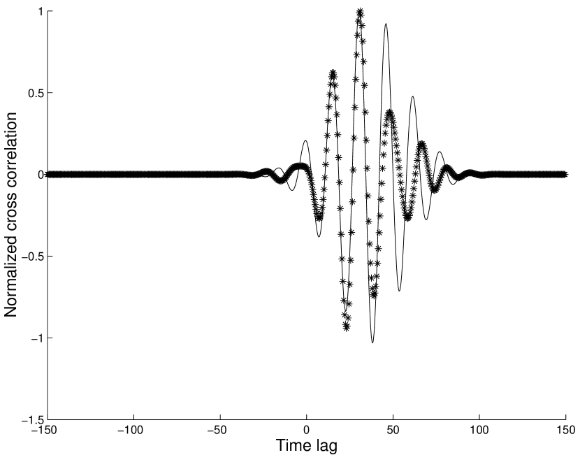
Figure 1: An example of the cross-covariance function normalized by its maximum value as a function of the time lag. The solid line represents no masking that is computed from equation (11), while the star (*) line represents the effect of masking, calculated from equation (45). It can been seen that there is a shift in the travel times as a result of masking.

The formula in equation (45) is the masked cross-covariance. There are few extra parameters that represent the shifts in the phase and group travel times, due to the masking process that depend on the angular positions of the mask function. The coefficients $q_{l}$ and $Q_{l}$ represent the functional form of the mask functions. Similar dependence is seen in (Rajaguru et al., 2006). A detailed numerical investigation of the amplitude modulation effects is outside the scope of this paper. In Figure 1, we just give an example of the expression in equation (45) plotted for a particular mask position and compared with equation (11) without masking. We observe shifts in the cross covariance and hence the travel times change due to the masking process. To investigate to effect of the shape of the mask function, different values of $Q_{l}$ need to be included when computing the sum in equation (46). In this derivation we assumed that the modulation function exhibits azimuthal symmetry. For a general modulation function, the analytical approach becomes difficult, and numerical methods must be employed.

In the model presented here, we assumed that the solar p modes have a narrow Gaussian amplitude function, that is peaked at $\omega_{o}$. Using this fact we evaluate the phase shift factor due to the horizontal component at this frequency (Nigam et al., 2007). Hence to a first order approximation, the phase shift is not affected by the masking procedure. In order to see the effect of masking on the horizontal component, we have to retain the frequency dependence of the phase shift factor when evaluating the integral in $\omega$. This will make the analytical approach intractable and the integral will have to be evaluated numerically.

3.2 Phase-speed filtering and amplitude modulation (masking) do not commute

In the previous section the signal $d^{x}(\vec{R},t)$ was first masked by $Q(\theta)$ and then phase speed filtered by $F_{p}(L,\omega_{nl})$. The signal is,

$$d_{f_{pQ}}^{x}(\vec{R},t)=\sum_{n,l,m}G_{l}(\omega_{nl})F_{p}(L,\omega_{nl})Q(\theta)d_{nlm}^{x}(\vec{R},t)$$ (47)

Expanding $Q(\theta)$ from equation (17) leads to

$$d_{f_{pQ}}^{x}(\vec{R},t)=\sum_{n,l,m}Q_{l}G_{l}(\omega_{nl})F_{p}(L,\omega_{nl})P_{l}(\cos\theta)d_{nlm}^{x}(\vec{R},t)$$ (48)

We immediately see that this corrupts the eigenfunction due to the $P_{l}(\cos\theta)$ term in the sum in equation (48) . The resulting cross-covariance was $\psi_{f_{pQ}}^{d^{x}}(\vec{R}_{1},\vec{R}_{2},\tau)$. We now reverse the order, first phase speed filter the signal $d^{x}(\vec{R},t)$ to get $d_{f_{p}}^{x}(\vec{R},t)$ and then mask to get $d_{f_{Qp}}^{x}(\vec{R}_{1},\vec{R}_{2},\tau)=Q(\theta)d_{f_{p}}^{x}(\vec{R},t)$. Computing the cross-covariance $\psi_{f_{Qp}}^{d^{x}}(\vec{R}_{1},\vec{R}_{2},\tau)$ for $d_{f_{Qp}}^{d^{x}}(\vec{R},t)$,

$$\psi_{f_{Qp}}^{d^{x}}(\vec{R}_{1},\vec{R}_{2},\tau)=\frac{1}{T}\int\limits_{0}^{T}d_{f_{Qp}}^{x}(\vec{R}_{1},t)\bar{d}_{f_{Qp}}^{x}(\vec{R}_{2},t+\tau)dt$$ (49)

This results in $\psi_{f_{Qp}}^{d^{x}}(\vec{R}_{1},\vec{R}_{2},\tau)=Q(\theta_{1})Q(\theta_{2})\psi_{f_{p}}^{d^{x}}(\vec{R}_{1},\vec{R}_{2},\tau)$, which is different from the expression for $\psi_{f_{pQ}}^{d^{x}}(\vec{R}_{1},\vec{R}_{2},\tau)$ in equation (22). Hence the order of masking and phase speed filtering are not interchangeable. Also we observe that phase speed filtering followed by masking results in the cross-covariance being just scaled in amplitude by the product of the mask functions $Q(\theta_{1})Q(\theta_{2})$, the travel times being unaffected by the process of masking. This is because masking changes the mode eigenfunctions due to the presence of an additional term $P_{l}(\cos\theta)$ in equation (48). Of course, the modified eigenfunctions no longer satisfy the original wave equation for solar oscillations. Thus, this procedure cannot be considered as a physical model of the amplitude variations observed in sunspots. Our calculations show that the phase-speed filtering procedure of the masked signal leads to spurious shifts in travel times due to mixing of different $l$ modes by the phase-speed filter. These shifts can occur if the masking is attributed to instrumental effects. However, this does not mean that the amplitude modulation due to the physical effects in sunspots results in similar effects in the travel-time measurements. This must be studied using realistic MHD models of sunspots.

3.3 Effect of Gaussian frequency filtering

Masking is observed only when the data is phase speed filtered after multiplying the signal with the mask function. In this section we show that just using a Gaussian frequency filter without a phase speed filter leads to no masking. Consider a masked signal $d_{Q}^{x}(\vec{R},t)$ that is filtered by a Gaussian frequency filter $G(\omega)=\exp\left(-{(\omega-\omega_{o})^{2}}/{\delta\omega^{2}}\right)$. The mask function $Q(\theta)$ is independent of $l$, and since the Gaussian frequency filter $G(\omega)$ does not depend on $l$, unlike the phase speed filter, the mask function $Q(\theta)$ can be pulled out of the sum in equation (50)

$$d_{f_{gQ}}^{x}(\vec{R},t)=\sum_{n,l,m}G(\omega_{nl})Q(\theta)d_{nlm}^{x}(\vec{R},t)=Q(\theta)d_{fg}^{x}(\vec{R},t)$$ (50)

where, $d_{fg}^{x}(\vec{R},t)=\sum_{n,l,m}G(\omega_{nl})d_{nlm}^{x}(\vec{R},t)$ is the signal filtered by a Gaussian frequency filter. We see that the frequency filtered signal $d_{fg}^{x}(\vec{R},t)$ is scaled by the mask function $Q(\theta)$, hence the cross-covariance $\psi_{f_{gQ}}^{d^{x}}(\vec{R}_{1},\vec{R}_{2},\tau)$ of $d_{f_{gQ}}^{x}(\vec{R},t)$ is

$$\psi_{f_{gQ}}^{d^{x}}(\vec{R}_{1},\vec{R}_{2},\tau)=Q(\theta_{1})Q(\theta_{2})\psi_{f_{g}}^{d^{x}}(\vec{R}_{1},\vec{R}_{2},\tau)$$ (51)

where, $\psi_{f_{g}}^{d^{x}}(\vec{R}_{1},\vec{R}_{2},\tau)$ is the cross-covariance of the Gaussian filtered signal $d_{fg}^{x}(\vec{R},t)$. We see that the effect of masking on the travel times is not observed in $\psi_{f_{gQ}}^{d^{x}}(\vec{R}_{1},\vec{R}_{2},\tau)$. It only undergoes a scaling of its amplitude by $Q(\theta_{1})Q(\theta_{2})$. So the effect of masking is not observed when the phase speed filter is absent, and we apply only a Gaussian frequency filter to the data.

4 Conclusion

In this paper we give an explanation as to why the localized spatial suppression or enhancement (masking) of the acoustic signal followed by phase speed filtering can appreciably shift the measured travel times, and cause systematic errors in time-distance inversions. Using only a frequency filter or reversing the operation of suppression (or enhancement) and phase speed filtering does not shift the travel times, but merely scales the cross covariance. Hence, the operations of masking and phase speed filtering are non-commutative. To explain this we develop a model and derive a new analytical formula for the cross-covariance in terms of the masking parameters, when the mask function has azimuthal symmetry. The reason for this is due to the fact that masking changes the spatial mode eigenfunctions, which when phase speed filtered, leads to a mixing of spatial modes, and is responsible for the travel time shifts. This may be useful to mimic amplitude changes in sunspots due to pure observational reasons, such as caused by altering the height of formation of the spectral line used for helioseismology measurements, and also to correct for the shifted travel times due to such effects. However, contrary to Rajaguru et al. (2006) suggestion, the procedure of masking oscillations of the quite Sun cannot model the amplitude reduction in sunspot due to physical mechanisms (e.g. changes in emissivity or wave absorption), and thus their recommendations of correcting the amplitude reduction by reversed masking may cause artificial shifts in observed travel times, and thus must be taken with caution.

References

• Chou et al. (2009) Chou, D.-Y., Liang, Z.-C., Yang, M.-H., Zhao, H., & Sun, M.-T.Β 2009, ApJ, 696, L106
• Christensen-Dalsgaard (2002) Christensen-Dalsgaard, J. 2002, Rev. Mod. Phys., 74, 1073
• Duvall et al. (1993) Duvall, T. L., Jr., Jeffries, S. M., Harvey, J. W., and Pomerantz, M. A. 1993, Nature, 362, 430
• Duvall et al. (1997) Duvall, T.Β L., Jr., et al.Β 1997, Sol.Β Phys., 170, 63
• Giles et al. (1997) Giles, P. M., Duvall, T. L., Jr., Scherrer, P. H., & Bogart, R. S. 1997, Nature, 390, 52
• Gradshteyn & Ryzhik (1994) Gradshteyn, I. S., & Ryzhik, I. M. 1994, page 531, Table of Integrals, Series, and Products, Academic Press, San Diego, fifth edition
• Jackson (1999) Jackson, J. D., 1999, Classical Electrodynamics, 3rd edition (New York: John Wiley & Sons)
• Kosovichev & Duvall (1997) Kosovichev, A. G., & Duvall, T. L. Jr., 1997, in F. Pijpers, J. Christensen Dalsgaard and C. S. Rosenthal (eds.), Solar Convection and Oscillations and Their Relationship, Proceedings of SCORe96 Workshop, pp 241-260, Kluwer, Dordrecht.
• Nigam et al. (2007) Nigam, R., Kosovichev, A.Β G., & Scherrer, P.Β H.Β 2007, ApJ, 659, 1736
• Parchevsky & Kosovichev (2007) Parchevsky, K.Β V., & Kosovichev, A.Β G.Β 2007, ApJ, 666, L53
• Rajaguru et al. (2006) Rajaguru, S. P., Birch, A. C., Duvall, T. L., Jr., Thompson, M. J., & Zhao, J. 2006, ApJ, 646, 543
• Zhao, Kosovichev, & Duvall (2001) Zhao, J., Kosovichev, A. G., & Duvall, T. L., Jr. 2001, ApJ, 557, 384
Refer to caption