Quantum Darwinism in non-ideal environments

Abstract

Quantum Darwinism provides an information-theoretic framework for the emergence of the objective, classical world from the quantum substrate. The key to this emergence is the proliferation of redundant information throughout the environment where observers can then intercept it. We study this process for a purely decohering interaction when the environment, $\mathcal{E}$, is in a non-ideal (e.g., mixed) initial state. In the case of good decoherence, that is, after the pointer states have been unambiguously selected, the mutual information between the system, $\mathcal{S}$, and an environment fragment, $\mathcal{F}$, is given solely by $\mathcal{F}$’s entropy increase. This demonstrates that the environment’s capacity for recording the state of $\mathcal{S}$ is directly related to its ability to increase its entropy. Environments that remain nearly invariant under the interaction with $\mathcal{S}$, either because they have a large initial entropy or a misaligned initial state, therefore have a diminished ability to acquire information. To elucidate the concept of good decoherence, we show that - when decoherence is not complete - the deviation of the mutual information from $\mathcal{F}$’s entropy change is quantified by the quantum discord, i.e., the excess mutual information between $\mathcal{S}$ and $\mathcal{F}$ is information regarding the initial coherence between pointer states of $\mathcal{S}$. In addition to illustrating these results with a single qubit system interacting with a multi-qubit environment, we find scaling relations for the redundancy of information acquired by the environment that display a universal behavior independent of the initial state of $\mathcal{S}$. Our results demonstrate that Quantum Darwinism is robust with respect to non-ideal initial states of the environment: the environment almost always acquires redundant information about the system but its rate of acquisition can be reduced.

I Introduction

Quantum mechanics was initially devised as a microscopic theory of atoms. However, macroscopic objects are made of quantum components. Thus quantum mechanics should describe our classical world as well. Yet, we do not observe “strange” quantum states in objects directly accessible to our senses. This has been a concern since the inception of quantum mechanics, even as its predictions continue to be verified. For many years, the strategy was - following Bohr - to bypass this difficulty by postulating a division between the classical and quantum worlds Bohr28-1 ; Bohr35-1 ; Wheeler83-1 ; Zurek91-1 .

The theory of decoherence is now the standard starting point for addressing these questions Zurek91-1 ; Zurek03-1 ; Joos03-1 ; Schlosshauer08-1 . A system coupled to an environment gets decohered into its pointer states Zurek81-1 ; Zurek03-1 that survive the interaction with the environment. This durability is one aspect of classicality. Amplification was also conjectured to play a role Bohr58-1 ; Zurek82-1 . Only very recently, however, has this role been made precise by the concept of redundancy in Quantum Darwinism, an information-theoretic framework for understanding the quantum-classical transition Ollivier04-1 ; Blume05-1 ; Zurek07-1 ; Brunner08-1 ; Bennett08-1 ; Paz09-1 ; Zwolak09-1 (see Ref. Zurek09-1 for a review). Within this framework, the objective, classical reality of the pointer states arises from the redundant dissemination of information about them throughout the environment. Many observers can then independently determine and reach consensus about the state of the system by intercepting separate fragments of the environment. This explains the “objective reality” of pointer states. They are not perturbed by measurements on the environment and, thus, as classical states should, they are immune to our “finding out” what they are. This process of discovery is especially easy when fragments of the environment do not interact with each other, e.g., such as photons. To make the analogy to Darwinism: certain states - the pointer states - “survive” the interaction with the environment and “procreate” by imprinting copies of themselves on the environment.

Quantum Darwinism is an extension of the decoherence paradigm, where now not only is the system of interest, but so is the environment. It acts as a witness to the state of the system and as a communication channel, transmitting information to observers. Previous studies on Quantum Darwinism focused on models where the system and environment are initially pure Ollivier04-1 ; Blume05-1 ; Paz09-1 . It is essential, however, to understand how different initial states influence the ability of the environment to effectively communicate information. A recent study has begun to examine the effect of starting with a “hazy” environment, i.e., one with some initial entropy. It was found that fairly hazy environments behave as noisy communication channels Zwolak09-1 . Here we go further by examining more generally how the environment’s capacity to transmit information is determined by its initial state and also distinguish between the transmission of quantum and classical information about the system (see also a recent work by Paz and Roncaglia that examines quantum and classical information in quantum Brownian motion Paz09-1 ).

We first outline, in Sec. II, the basic concepts behind Quantum Darwinism, including the mutual information that is used to compute the redundancy of information about the system in the environment. In Sec. III, we prove, in the typical case of good decoherence, that the mutual information between the system and a fragment of the environment is given by the fragment’s entropy increase when the system interacts independently with many components of the environment. In Sec. IV, we elucidate the concept of good decoherence by showing that - when decoherence is not complete - the deviation of the mutual information from the fragment’s entropy change is quantified by the quantum discord Zurek00-1 ; Henderson01-1 ; Ollivier02-1 . The excess mutual information between the system and the environment fragment is information about the initial coherent superposition of pointer states of the system.

After these general results, in Sec. V, we introduce a symmetric environment model composed of qubits that we use to illustrate the analytic results of Sec. III and IV. We demonstrate how classical information proliferates into the environment. Also, we investigate the dependence of the redundancy of classical information storage to hazy (i.e., mixed) and misaligned (e.g., close to an eigenstate of the interaction Hamiltonian) initial environment states. Starting with these non-ideal initial conditions diminishes the environment’s capacity to acquire and transmit information. For example, in a fairly hazy environment, the redundancy behaves as $1-h$ as $h\to 1$, where the haziness, $h$, is the initial entropy of an environment qubit. That is, it behaves as a noisy communication channel. For both hazy and misaligned environments we develop scaling relations for the behavior of the redundancy. These relations show a universal behavior of the redundancy that is independent of the initial state of the system. In Appendix A, we solve for the mutual information and discord for several parameter regimes of the symmetric environment model. In Appendix B, we outline a numerically exact procedure for computing the entropies (that show up in the mutual information) for the model. In Appendix C, we derive an approximate expression for the mutual information that elucidates the behavior of the redundancy.

II Information and Redundancy

Quantum Darwinism recognizes and investigates the ability of the environment to redundantly record information about a “system of interest.” As before Ollivier04-1 ; Blume05-1 ; Zwolak09-1 ; Paz09-1 , we focus on the mutual information

$$I(\mathcal{S}:\mathcal{F})=H_{\mathcal{S}}(t)+H_{\mathcal{F}}(t)-H_{\mathcal{S}\mathcal{F}}(t)$$ (1)

between the system, $\mathcal{S}$, and a fragment $\mathcal{F}$ of the environment $\mathcal{E}$. Above, $H_{\mathcal{S}}(t)$ and $H_{\mathcal{F}}(t)$ are the von Neumann entropies at time $t$ of $\mathcal{S}$ and $\mathcal{F}$, respectively, and $H_{\mathcal{S}\mathcal{F}}(t)$ is the joint entropy $\mathcal{S}$ and $\mathcal{F}$. The mutual information between $\mathcal{S}$ and $\mathcal{F}$ quantifies the correlations between the two. When $\mathcal{S}$ and $\mathcal{F}$ are initially uncorrelated, $I\left(\mathcal{S}:\mathcal{F}\right)$ gives the total information $\mathcal{F}$ gained about the state of $\mathcal{S}$.

We want to investigate how much information $\mathcal{F}$ acquires about $\mathcal{S}$ when they interact and how redundant this information is. We do not insist on acquiring all of the missing classical information, $H_{\mathcal{S}}$, about the system: The information deficit $\delta$ is the fraction of $H_{\mathcal{S}}$ we are prepared to forgo. For a given $\delta$, the redundancy of information about $\mathcal{S}$ is the maximum number of disjoint fragments $R_{\delta}$ that have a mutual information greater than $\left(1-\delta\right)H_{\mathcal{S}}$ with $\mathcal{S}$. In terms of a fragment size, the redundancy is

$$R_{\delta}=\frac{{{}^{\sharp}}\mathcal{E}}{{{}^{\sharp}}\mathcal{F}_{\delta}}=\frac{1}{f_{\delta}},$$ (2)

where the environment has ${{}^{\sharp}}\mathcal{E}$ components, ${{}^{\sharp}}\mathcal{F}_{\delta}$ is the typical size of an environment fragment needed to acquire a mutual information no less than $\left(1-\delta\right)H_{\mathcal{S}}$, and $f_{\delta}={{}^{\sharp}}\mathcal{E}/{{}^{\sharp}}\mathcal{F}_{\delta}$ is the corresponding fraction of the environment. In the symmetric environment considered in Sec. V all possible partitions of the environment into fragments of size ${{}^{\sharp}}\mathcal{F}_{\delta}$ have identical mutual information and, thus, ${{}^{\sharp}}\mathcal{F}_{\delta}$ is the size of the environment fragment needed to give $I\left(\mathcal{S}:\mathcal{F}\right)\geq\left(1-\delta\right)H_{\mathcal{S}}$.

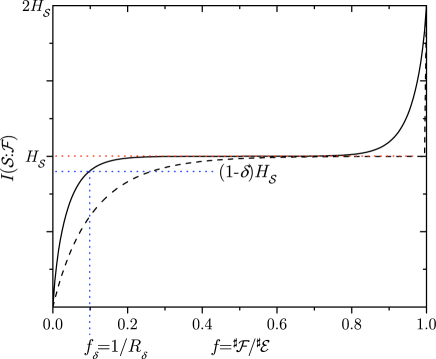
Figure 1: The behavior of the mutual information, $I\left(\mathcal{S}:\mathcal{F}\right)$, between the system, $\mathcal{S}$, and a fragment, $\mathcal{F}$, of a symmetric environment, $\mathcal{E}$, as a function of the fraction of the environment intercepted, $f={{}^{\sharp}}\mathcal{F}/{{}^{\sharp}}\mathcal{E}$. The black solid line is for an initially pure $\mathcal{E}$ and the black dashed line is for an initially hazy $\mathcal{E}$. Here, ${{}^{\sharp}}\mathcal{F}$ and ${{}^{\sharp}}\mathcal{E}$ are the number of components in the fragment and the environment, respectively. The information $H_{\mathcal{S}}$ sets the limit of classical information about $\mathcal{S}$ that $\mathcal{E}$ can acquire, resulting in a plateau region at $H_{\mathcal{S}}$ (the classical plateau) that signifies the redundant proliferation of classical information into the environment. We define a fragment size, ${{}^{\sharp}}\mathcal{F}_{\delta}$, that gives the value of the mutual information $\left(1-\delta\right)H_{\mathcal{S}}$, i.e., to within the information deficit, $\delta$, of the classical plateau. The redundancy, $R_{\delta}$, at this information deficit is then given by Eq. (2). The initial haziness of $\mathcal{E}$ reduces the redundancy. The data for this figure is from an actual simulation like those performed in Sec. V.

The mutual information given by Eq. (1) and redundancy given by Eq. (2) set the stage for studying how information is acquired by the environment. Previous studies have shown the formation of a classical plateau with $I\left(\mathcal{S}:\mathcal{F}\right)\simeq H_{\mathcal{S}}$. Figure 1 shows an example of this type of behavior and clarifies the quantities involved in defining the redundancy.

III Information capacity of a purely decohering environment

In this section and the following section, we prove two general results about how purely decohering environments store and transmit information. We consider a general model of pure decoherence given by the Hamiltonian

$$\mathbf{H}_{\mathcal{S}\mathcal{E}}=\sum_{k=1}^{{{}^{\sharp}}\mathcal{E}}\Pi_{\mathcal{S}}\Upsilon_{k},$$ (3)

where $\Pi_{\mathcal{S}}$ is a Hermitian operator on $\mathcal{S}$ and $\Upsilon_{k}$ is a Hermitian operator on the $k^{th}$ environment component . This Hamiltonian does not generate transitions between the pointers states, given by the eigenstates of $\Pi_{\mathcal{S}}$, of the system. In this model of many environment components interacting independently with $\mathcal{S}$, we consider a product initial state

$$\rho\left(0\right)=\rho_{\mathcal{S}}\left(0\right)\otimes\left[\bigotimes_{k=1}^{{{}^{\sharp}}\mathcal{E}}\rho_{k}\left(0\right)\right].$$ (4)

To compute the mutual information, we calculate the entropies of $\rho_{\mathcal{S}}\left(t\right)$, $\rho_{\mathcal{F}}\left(t\right)$, and $\rho_{\mathcal{S}\mathcal{F}}\left(t\right)$. Here, however, we want to first show how the mutual information can be written more transparently by replacing the entropy of $\rho_{\mathcal{S}\mathcal{F}}(t)$ with the sum of two entropies: $\rho_{\mathcal{S}}$ decohered only by the remainder of the environment, $\mathcal{E}/\mathcal{F}$, and $\rho_{\mathcal{F}}\left(0\right)$. That is, the state

$$\rho_{\mathcal{S}\mathcal{F}}\left(t\right) = \mathrm{tr}_{\mathcal{E}/\mathcal{F}}\left[e^{-\imath\mathbf{H}_{\mathcal{S}\mathcal{E}}t}\rho\left(0\right)e^{\imath\mathbf{H}_{\mathcal{S}\mathcal{E}}t}\right]$$ (5)

$$= e^{-\imath\mathbf{H}_{\mathcal{S}\mathcal{F}}t}\left\{\mathrm{tr}_{\mathcal{E}/\mathcal{F}}\left[e^{-\imath\mathbf{H}_{\mathcal{S}\mathcal{E}/\mathcal{F}}t}\rho_{\mathcal{S}\mathcal{E}/\mathcal{F}}\left(0\right)e^{\imath\mathbf{H}_{\mathcal{S}\mathcal{E}/\mathcal{F}}t}\right]\otimes\rho_{\mathcal{F}}\left(0\right)\right\}e^{\imath\mathbf{H}_{\mathcal{S}\mathcal{F}}t},$$

where $\mathbf{H}_{\mathcal{S}\mathcal{F}}=\sum_{k\in\mathcal{F}}\Pi_{\mathcal{S}}\Upsilon_{k}$ and $\mathbf{H}_{\mathcal{S}\mathcal{E}/\mathcal{F}}=\sum_{k\in\mathcal{E}/\mathcal{F}}\Pi_{\mathcal{S}}\Upsilon_{k}$, has the same entropy as

$$\rho_{\mathcal{S}d\left(\mathcal{E}/\mathcal{F}\right)}(t)\otimes\rho_{\mathcal{F}}\left(0\right).$$ (6)

Here $\mathcal{S}d\left(\mathcal{E}/\mathcal{F}\right)$ is the system decohered solely by $\mathcal{E}/\mathcal{F}$ (i.e., evolved only by the Hamiltonian $\mathbf{H}_{\mathcal{S}\mathcal{E}/\mathcal{F}}$) and $\rho_{\mathcal{F}}\left(0\right)=\bigotimes_{k\in\mathcal{F}}\rho_{k}\left(0\right)$ is the initial state of $\mathcal{F}$. Hence the entropy of $\rho_{\mathcal{S}\mathcal{F}}(t)$ is

$$H_{\mathcal{S}\mathcal{F}}(t)=H_{\mathcal{S}d\left(\mathcal{E}/\mathcal{F}\right)}(t)+H_{\mathcal{F}}(0).$$ (7)

Therefore, the mutual information is

$$I\left(\mathcal{S}:\mathcal{F}\right)=\left[H_{\mathcal{F}}(t)-H_{\mathcal{F}}(0)\right]+\left[H_{\mathcal{S}d\mathcal{E}}(t)-H_{\mathcal{S}d\left(\mathcal{E}/\mathcal{F}\right)}(t)\right],$$ (8)

where $H_{\mathcal{S}d\mathcal{E}}(t)=H_{\mathcal{S}}(t)$, i.e., $H_{\mathcal{S}d\mathcal{E}}(t)$ is $\mathcal{S}$ decohered by the whole environment $\mathcal{E}$ . The first term in brackets in Eq. (8) is the entropy increase of the fragment $\mathcal{F}$ due to the interaction with $\mathcal{S}$. The second term is the difference of the entropy of $\mathcal{S}$ interacting with all of $\mathcal{E}$ and the entropy of $\mathcal{S}$ interacting solely with $\mathcal{E}/\mathcal{F}$. When both $\mathcal{E}$ and $\mathcal{E}/\mathcal{F}$ are sufficient to decohere $\mathcal{S}$ at a given time, the second term, $H_{\mathcal{S}d\mathcal{E}}(t)-H_{\mathcal{S}d\left(\mathcal{E}/\mathcal{F}\right)}(t)$, will be nearly zero. This will happen when $\mathcal{E}$ has decohered $\mathcal{S}$ and the size of $\mathcal{F}$ is small compared to the size of $\mathcal{E}$. This approximation of good decoherence is accurate at all but very short times (i.e., less than the decoherence time ) or for very large fragments (i.e., when the size of $\mathcal{E}/\mathcal{F}$ is too small to decohere $\mathcal{S}$). Thus, in the typical case of good decoherence, the mutual information will be approximately

$$I\left(\mathcal{S}:\mathcal{F}\right)\approx H_{\mathcal{F}}(t)-H_{\mathcal{F}}(0).$$ (9)

This reduces to just $I\left(\mathcal{S}:\mathcal{F}\right)\approx H_{\mathcal{F}}\left(t\right)$ for initially pure environments Zurek07-1 . The mutual information rewritten as in Eq. (9) is a universal relationship for any “decoherence only” model where $\mathcal{S}$ interacts with independent environment components and where good decoherence has taken place.

From Eq. (9), it is clear that when $\mathcal{F}$ starts in a state that commutes with $\mathbf{H}_{\mathcal{S}\mathcal{F}}$, i.e., diagonal in the basis of the interaction operator that appears in $\mathbf{H}_{\mathcal{S}\mathcal{F}}$ (either because it is mixed in that basis or starts in one of the eigenstates of that basis), it has no capacity to increase its entropy and therefore no capacity to store classical information about $\mathcal{S}$. In other words, states of $\mathcal{E}$ that remain invariant under the Hamiltonian dynamics generated by Eq. (3) do not redundantly store information about $\mathcal{S}$. The extent to which the environment’s initial state coincides with such states degrades its transmission capabilities.

IV Discord and Decoherence

In this section, we show that before good decoherence has been reached (or for sufficiently large $\mathcal{F}$), the second term in Eq. (8) contributes to the mutual information. This second term is the quantum discord Zurek00-1 ; Henderson01-1 ; Ollivier02-1 with respect to the pointer basis of $\mathcal{S}$. The quantum discord with respect to any basis, $\left\{\Pi_{\mathcal{S}}\right\}$, is defined as the difference between two classically equivalent expressions for the mutual information Ollivier02-1 :

$$\boldsymbol{\delta}\left(\mathcal{S}:\mathcal{F}\right)_{\left\{\Pi_{\mathcal{S}}\right\}} = I\left(\mathcal{S}:\mathcal{F}\right)-J\left(\mathcal{S}:\mathcal{F}\right)_{\left\{\Pi_{\mathcal{S}}\right\}}$$ (10)

$$= H_{\mathcal{S}}(t)-H_{\mathcal{S}\mathcal{F}}(t)+H_{\mathcal{F}\left|\left\{\Pi_{\mathcal{S}}\right\}\right.}(t).$$ (11)

Above,

$$J\left(\mathcal{S}:\mathcal{F}\right)_{\left\{\Pi_{\mathcal{S}}\right\}}=H_{\mathcal{F}}(t)-H_{\mathcal{F}\left|\left\{\Pi_{\mathcal{S}}\right\}\right.}(t)$$ (12)

is the other classical expression for the mutual information in terms of the conditional information (i.e., the entropy decrease of $\mathcal{F}$ given a measurement of $\Pi_{\mathcal{S}}$ on $\mathcal{S}$) .

The second term in brackets in Eq. (8) is the quantum discord with respect to the pointer basis of $\mathcal{S}$, i.e., the eigenbasis of $\Pi_{\mathcal{S}}$ from the Hamiltonian in Eq. (3) . To show this, we first rewrite the quantum discord using Eq. (7) as

$$\boldsymbol{\delta}\left(\mathcal{S}:\mathcal{F}\right)_{\left\{\Pi_{\mathcal{S}}\right\}} = H_{\mathcal{S}d\mathcal{E}}(t)-H_{\mathcal{S}d\left(\mathcal{E}/\mathcal{F}\right)}(t)$$ (13)

$$-H_{\mathcal{F}}(0)+H_{\mathcal{F}\left|\left\{\Pi_{\mathcal{S}}\right\}\right.}(t).$$

The last term, however, simplifies to

$$H_{\mathcal{F}\left|\left\{\Pi_{\mathcal{S}}\right\}\right.}(t) = \sum_{j}p_{j}H_{\mathcal{F}\left|\Pi_{j}^{\mathcal{S}}\right.}(t)$$ (14)

$$= \sum_{j}p_{j}H\left(\mathcal{U}_{j}\rho_{\mathcal{F}}\left(0\right)\mathcal{U}_{j}^{\dagger}\right)$$ (15)

$$= H_{\mathcal{F}}(0),$$ (16)

where $p_{j}$ is the occupation of the $j^{th}$ eigenstate of $\Pi_{\mathcal{S}}$ and $\mathcal{U}_{j}$ is the evolution operator projected onto that state. Thus, in this case of pure decoherence by independent environment components, the quantum discord is

$$\boldsymbol{\delta}\left(\mathcal{S}:\mathcal{F}\right)_{\left\{\Pi_{\mathcal{S}}\right\}}=H_{\mathcal{S}d\mathcal{E}}(t)-H_{\mathcal{S}d\left(\mathcal{E}/\mathcal{F}\right)}(t).$$ (17)

The discord represents information complementary to the information about the pointer states of $\mathcal{S}$ that the environment fragment has acquired. To see this, note that the discord in Eq. (17) involves only the entropy of $\mathcal{S}$ evolved in the presence of the full environment $\mathcal{E}$ and the environment without the fragment $\mathcal{E}/\mathcal{F}$. Under a pure decoherence Hamiltonian, any difference between these two is due to off-diagonal elements in the system’s initial density matrix. That is, the discord yields information about the initial coherence between pointer states of $\mathcal{S}$. This is information about the complementary observables to $\Pi_{\mathcal{S}}$, i.e., operators that do not commute with $\Pi_{\mathcal{S}}$.

In pure decoherence models, the same complementary information flows into the environment regardless of whether $\mathcal{E}$ is in an initially pure or mixed state. This comes out of Eq. (17) after recognizing that the environment decoheres the system identically regardless of its initial entropy when its alignment is held fixed.. However, even though the initial entropy of the environment does not effect its ability to receive complementary information, its alignment with the states that commute with $\mathbf{H}_{\mathcal{S}\mathcal{E}}$ does effect this ability. These issues will be discussed along with the following concrete, solvable example in order to elucidate the ideas shown here.

V Example: Qubit interacting with a symmetric environment

We now study a solvable example of a qubit system interacting with a symmetric qubit environment often used as a model of decoherence Zurek81-1 ; Zurek82-1 . The Hamiltonian is

$$\mathbf{H}_{\mathcal{S}\mathcal{E}}=\frac{1}{2}\sum_{k=1}^{{{}^{\sharp}}\mathcal{E}}\sigma_{\mathcal{S}}^{z}\sigma_{k}^{z}.$$ (18)

It causes pure decoherence of the system’s state into its pointer basis - the eigenstates of $\sigma_{\mathcal{S}}^{z}$. In this basis, the system is initially described by

$$\rho_{\mathcal{S}}(0)=\left(\begin{array}[]{cc}s_{00}&s_{01}\\ s_{10}&s_{11}\end{array}\right).$$ (19)

We take the initial state of the environment to be the product state, Eq. (4), with $\rho_{k}\left(0\right)=\rho_{r}$ for all $k$. In the $\sigma^{z}$ basis, the density matrix of each component is

$$\rho_{r}=\left(\begin{array}[]{cc}r_{00}&r_{01}\\ r_{10}&r_{11}\end{array}\right).$$ (20)

We examine how two quantities that characterize this state, its haziness and misalignment, affect its ability to accept information. Figure 2 shows a representation of these quantities using the Bloch sphere. The haziness is the preexisting entropy of an environment qubit:

$$h\equiv H\left(\rho_{r}\right).$$ (21)

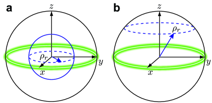
Figure 2: Bloch sphere representation of (a) haziness and (b) misalignment. Pure states in the x-y plane (highlighted) have the maximum capacity to accept information about the system’s pointer states. Haziness of an environment qubit contracts its Bloch sphere, reducing the qubits ability to increase its entropy and therefore decreasing its capacity to store information. Misalignment rotates the state out of the x-y plane, which also decreases the qubits capacity to store information. For both haziness and misalignment, the decrease in capacity is due to a reduction in the environment qubits’ ability to branch into two orthogonal states correlated with the two pointer states of the system.

Misalignment of a component of the environment is tilting it away from the states that have the most capacity to accept information. Thus, we can similarly define the misalignment of the environment by the maximum entropy it can obtain under a pure decoherence Hamiltonian,

$$h_{m}\equiv H\left(r_{00}\right),$$ (22)

where $H(x)\equiv-x\log_{2}x-\left(1-x\right)\log_{2}(1-x)$ is the binary entropy. This parameter indicates the maximum amount of information (according to Eq. (9)) that an environment qubit can ever obtain after good decoherence has taken place under the evolution of Eq. (18). The maximum capacity states are qubits that start in the $x-y$ plane of the Bloch sphere. The minimum capacity states are $\sigma^{z}$ eigenstates, which will not even decohere $\mathcal{S}$. When we calculate the redundancy, however, we find it more convenient to parametrize the misalignment of $\rho_{r}$ as

$$\sigma=r_{00}-r_{11}$$ (23)

instead of using Eq. (22). When an environment qubit is in a $\sigma^{z}$ eigenstate, $\left|\sigma\right|=1$, it will remain untouched by $\mathbf{H}_{\mathcal{S}\mathcal{E}}$ of Eq. (18). The details of the calculations can be found in the appendices. In the following we highlight the main results.

V.1 Mutual Information

In Appendix A and using Eq. (8), we show that the mutual information takes on the form

$$I\left(\mathcal{S}:\mathcal{F}\right) = \left[H_{\mathcal{F}}\left(t\right)-H_{\mathcal{F}}\left(0\right)\right]$$ (24)

$$+\left[H\left(\kappa_{\mathcal{E}}(t)\right)-H\left(\kappa_{\mathcal{E}/\mathcal{F}}(t)\right)\right],$$

where

$$\kappa_{\mathcal{A}}(t)=\frac{1}{2}\left(1+\sqrt{\left(s_{11}-s_{00}\right)^{2}+4\left|s_{01}\right|^{2}\left|\Lambda_{\mathcal{A}}(t)\right|^{2}}\right)$$ (25)

and $\Lambda_{\mathcal{A}}(t)$ is the contribution to decoherence of $\mathcal{S}$ due to the subset $\mathcal{A}$ of the environment. Figures 3(a,b) and 4(a,b) show the behavior of the mutual information versus time for several different cases involving pure and mixed $\mathcal{S}$ and pure, mixed, and misaligned $\mathcal{E}$.

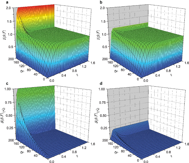
Figure 3: (a,b) Mutual information, $I\left(\mathcal{S}:\mathcal{F}\right)$, and (c,d) Quantum discord, $\boldsymbol{\delta}\left(\mathcal{S}:\mathcal{F}\right)_{\left\{\sigma_{\mathcal{S}}^{z}\right\}}$, versus the fragment size, ${{}^{\sharp}}\mathcal{F}$, and time, $t$, with $s_{00}=1/2$, $r_{00}=1/2$, and ${{}^{\sharp}}\mathcal{E}=200$. (a,b) The mutual information for $H_{\mathcal{S}}(0)=0$ and $H_{\mathcal{S}}(0)=0.8$, respectively. Initially $\mathcal{E}$ and $\mathcal{S}$ are uncorrelated, but as time develops, $\mathcal{E}$ acquires information about $\mathcal{S}$. After an initial transient region - signified by a nonzero quantum discord in (c,d) - a plateau develops in the mutual information. A sudden increase in the von Neumann mutual information occurs for large ${{}^{\sharp}}\mathcal{F}\sim{{}^{\sharp}}\mathcal{E}$ because complementary information about $\mathcal{S}$ is accessible via global measurements. For a system initially in a superposition, this jump is large and so is the discord in the transient region. The jump is reduced by any existing decoherence of $\mathcal{S}$ when it is placed in contact with $\mathcal{E}$. However, the level and size of the classical plateau is identical regardless of the initial entropy of $\mathcal{S}$. (c,d) The quantum discord with respect to the eigenstates of $\Pi_{\mathcal{S}}=\sigma_{\mathcal{S}}^{z}$ for $H_{\mathcal{S}}(0)=0$ and $H_{\mathcal{S}}(0)=0.8$, respectively. The environment, $\mathcal{E}$, can be pure or mixed, and, in fact, the discord is equivalent to the mutual information between $\mathcal{S}$ and $\mathcal{F}$ for a diagonal initial state $\rho_{r}$. There is a transient region, just after $\mathcal{S}$ and $\mathcal{E}$ have come into contact, where nonzero discord exists. Its duration depends on the size of the environment. Except for this region, the discord is negligibly small since both $\mathcal{E}$ and $\mathcal{E}/\mathcal{F}$ are sufficient to decohere $\mathcal{S}$. The discord is reduced by the preexisting entropy of $\mathcal{S}$ before coming in contact with $\mathcal{E}$, as shown in (b). This is because the discord signifies complementary information about $\mathcal{S}$, i.e., information about the initial coherence between pointer states of $\mathcal{S}$.

For pure $\mathcal{S}$ and pure $\mathcal{E}$, the mutual information is plotted in Fig. 3(a). Initially $\mathcal{S}$ and $\mathcal{E}$ are uncorrelated and therefore the environment contains no information about the system. In time, however, correlations begin to encode information about both the pointer states of $\mathcal{S}$ and their superpositions. The latter is reflected by the nonzero quantum discord in Fig. 3(c,d). After good decoherence has taken place, a plateau develops in the mutual information as a function of ${{}^{\sharp}}\mathcal{F}$. This classical plateau signifies classical (i.e., redundant and therefore objective) information that has proliferated throughout the environment.

For mixed $\mathcal{S}$ and pure $\mathcal{E}$, the mutual information is plotted in Fig. 3(b) for $H_{\mathcal{S}}(0)=0.8$. As with a pure $\mathcal{S}$, the environment develops correlations with the system. In particular, it obtains information about the pointer states of the system. Thus, as before, the classical plateau forms at the same level, $H_{\mathcal{S}}$, which is determined only by diagonal elements of the system’s initial density matrix in its pointer basis. However, the available complementary information about $\mathcal{S}$, as signified by the discord with $\mathcal{F}$, is reduced due to the initial entropy of $\mathcal{S}$.

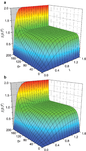
Figure 4: Mutual information, $I\left(\mathcal{S}:\mathcal{F}\right)$, versus the fragment size, ${{}^{\sharp}}\mathcal{F}$, and time, $t$, for an initially pure $\mathcal{S}$ and (a) an initially hazy $\mathcal{E}$ with $r_{00}=1/2$ and $h\approx 0.8$, and (b) an initially hazy and misaligned $\mathcal{E}$ with $\sigma=0.8$ and $h/h_{m}\approx 0.8$. The other parameters are $s_{00}=1/2$ and ${{}^{\sharp}}\mathcal{E}=200$. As with Fig. 3, $\mathcal{E}$ initially contains no information about $\mathcal{S}$, but correlations develop, transmitting information about $\mathcal{S}$ throughout $\mathcal{E}$, then going over to a classical regime signified by the formation of the classical plateau. Misalignment and haziness both reduce the information a given fragment $\mathcal{F}$ gains about $\mathcal{S}$. However, since the classical plateau forms, the environment still maintains the ability to redundantly encode classical information about $\mathcal{S}$.

Environments, however, will generally contain some preexisting entropy, e.g., due to a finite temperature or interactions with other degrees of freedom not directly in contact with $\mathcal{S}$ (for example, photons emitted from the sun are initially partially mixed). In Fig. 4, the mutual information is plotted for a hazy environment, $h\approx 0.8$, and a hazy, misaligned environment with $\sigma=0.8$ and $h/h_{m}\approx 0.8$ . Although the classical plateau is slower to develop as a function of ${{}^{\sharp}}\mathcal{F}$, it still forms at the same level, $H_{\mathcal{S}}$, as for an initially pure $\mathcal{E}$. This is significant, as it shows that the pointer states of $\mathcal{S}$ can still be completely determined from a fragment of $\mathcal{E}$ even when the environment is initially in a non-ideal state.

V.2 Discord

The second term in brackets in Eq. (24) gives the quantum discord with respect to the eigenstates of $\sigma_{\mathcal{S}}^{z}$:

$$\boldsymbol{\delta}\left(\mathcal{S}:\mathcal{F}\right)_{\left\{\sigma_{\mathcal{S}}^{z}\right\}}=H\left(\kappa_{\mathcal{E}}(t)\right)-H\left(\kappa_{\mathcal{E}/\mathcal{F}}(t)\right),$$ (26)

which is plotted in Fig. 3(c,d) for two initial conditions. This is the deviation from the good decoherence expression, Eq. (9), for the mutual information. This deviation term will be nearly zero whenever $\kappa_{\mathcal{E}}(t)\approx\kappa_{\mathcal{E}/\mathcal{F}}(t)$, which occurs when $\left|\Lambda_{\mathcal{E}}(t)-\Lambda_{\mathcal{E}/\mathcal{F}}(t)\right|\approx 0$ - that is, whenever both $\mathcal{E}$ and $\mathcal{E}/\mathcal{F}$ are sufficient to decohere $\mathcal{S}$ . In this symmetric model, good decoherence means that both ${{}^{\sharp}}\mathcal{E}$ and ${{}^{\sharp}}\mathcal{E}-{{}^{\sharp}}\mathcal{F}$ are sufficiently large, or that $\Lambda_{k}(t)$, the contribution of a single $\mathcal{E}$ spin to decoherence (see Eq. (39)), is sufficiently small, so the decoherence factors $\Lambda_{\mathcal{E}}(t)$ and $\Lambda_{\mathcal{E}/\mathcal{F}}(t)$ are both small.

As discussed above, the discord represents information the environment fragment has acquired regarding complementary observables of $\mathcal{S}$. In this qubit system with a $\sigma_{\mathcal{S}}^{z}$ pointer basis, the complementary observables are $\sigma_{\mathcal{S}}^{x}$ and $\sigma_{\mathcal{S}}^{y}$. The initial expectation value of these observables are $\langle\sigma_{\mathcal{S}}^{x}\rangle_{0}=2\Re s_{01}$ and $\langle\sigma_{\mathcal{S}}^{y}\rangle_{0}=-2\Im s_{01}$, respectively. Since the discord is the difference of two terms, which only differ by the factor multiplying $s_{01}$, it contains information regarding the initial expectation value of $\sigma_{\mathcal{S}}^{x}$ and $\sigma_{\mathcal{S}}^{y}$, whereas the first term in brackets in Eq. (24) does not (as can be seen from the form of $\rho_{\mathcal{F}}(t)$ in Eq. (43)). This is more obvious close to good decoherence when the discord becomes

$$\boldsymbol{\delta}\left(\mathcal{S}:\mathcal{F}\right)_{\left\{\sigma_{\mathcal{S}}^{z}\right\}} \approx \left(\langle\sigma_{\mathcal{S}}^{x}\rangle_{0}^{2}+\langle\sigma_{\mathcal{S}}^{y}\rangle_{0}^{2}\right)\times$$

$$\left(\left|\Lambda_{\mathcal{E}/\mathcal{F}}(t)\right|^{2}-\left|\Lambda_{\mathcal{E}}(t)\right|^{2}\right)\frac{\log_{2}\left(s_{00}/s_{11}\right)}{4\left(s_{11}-s_{00}\right)}.$$

That is, the quantum discord is directly proportional to the expectation value of the observables that do not commute with the pointer observable $\sigma_{\mathcal{S}}^{z}$.

Equation (26) together with Eq. (25) also show that whether the environment is pure or hazy, it acquires identical complementary information about $\mathcal{S}$. This is evident by the dependence of the quantum discord only on how $\mathcal{E}$ and $\mathcal{E}/\mathcal{F}$ decohere $\mathcal{S}$. The latter only relies on the initial alignment of the environment components with the eigenstates of $\sigma^{z}$, but not on how hazy they are.

V.3 Redundancy

In the previous two subsections we examined the behavior of the mutual information and quantum discord in various parameter regimes. We now examine the behavior of the redundancy for different initial states of the system and environment.

Hazy $\mathcal{E}$ - As discussed above, an initially hazy $\mathcal{E}$ has a lower capacity to store information Zwolak09-1 . In Fig. 5(a,b), we plot the mutual information versus ${{}^{\sharp}}\mathcal{F}$ and $h$ at $t=\pi/2$ and $t=\pi/4$. Even though the initial haziness diminishes the capacity of the environment to acquire and transmit information, we see that the classical plateau still forms and at the same level ($H_{\mathcal{S}}$), but takes a longer time to develop and flattens out only for larger ${{}^{\sharp}}\mathcal{F}$. Moreover, the final jump of the mutual information when ${{}^{\sharp}}\mathcal{F}\approx{{}^{\sharp}}\mathcal{E}$, which signifies complete quantum correlation of $\mathcal{E}$ with $\mathcal{S}$, is the same regardless of whether the environment is initially pure or hazy. Somewhat surprisingly, it occurs even for a completely hazy environment ($h=1$) where the classical plateau is missing. Thus the complementary information about $\mathcal{S}$ remains the same regardless of the haziness, $h$, at fixed misalignment.

In Fig. 5(c), we plot the redundancy for $t=\pi/2$ and $t=\pi/4$. This shows explicitly that although the capacity of the environment is reduced, the redundancy is still large. There is an initial, more rapid drop in the redundancy as the state becomes a little hazy, but this crosses over to a linear region where redundancy behaves as $1-h$, i.e., like a noisy communication channel Cover06-1 . The initial, more rapid drop at $t=\pi/2$ is due to the symmetry of the environment: when $h=0$ each qubit has complete classical correlation with $\mathcal{S}$.

In Appendix C, we derive an approximate expression for the mutual information at $r_{00}=1/2$ and $t=\pi/2$ for fairly hazy $\mathcal{E}$ and large ${{}^{\sharp}}\mathcal{F}$:

$$I\left(\mathcal{S}:\mathcal{F}\right)\approx H_{\mathcal{S}}-\frac{\left(2\sqrt{\lambda_{-}\lambda_{+}}\right)^{{{}^{\sharp}}\mathcal{F}}}{\sqrt{\pi{{}^{\sharp}}\mathcal{F}/2}}\frac{2\pi\sqrt{s_{00}s_{11}}}{\left(\ln 2\right)\left(\ln\frac{\lambda_{+}}{\lambda_{-}}\right)}.$$ (28)

This asymptotic expression allows us to estimate the redundancy when the information deficit, $\delta$, is small as

$$R_{\delta}\approx\frac{{{}^{\sharp}}\mathcal{E}\ln\left(2\sqrt{\lambda_{-}\lambda_{+}}\right)}{\ln\delta}.$$ (29)

This expression is plotted in Fig. 5(c) along with the exact data (and also the linear approximation) for $t=\pi/2$. Even when ${{}^{\sharp}}\mathcal{F}_{\delta}$ is small (i.e., for small information deficits and haziness), this approximation captures the behavior of the redundancy . As $\delta\to 0$, the redundancy for an arbitrary initial system state collapse onto this same universal curve. Thus, we define a limiting redundancy

$$\bar{R}=\lim_{\delta\to 0}\frac{-R_{\delta}\ln\delta}{{{}^{\sharp}}\mathcal{E}}.$$ (30)

This expression, with $R_{\delta}$ from Eq. (29), is shown in Fig. 5(d) along with $\bar{R}$ from the exact data for four different initial states of $\mathcal{S}$: $s_{00}=1/2$, $s_{00}=1/8$, $s_{00}=1/64$, and $s_{00}=1/4096$. From the figure, we see that when discrete effects disappear, the limiting redundancy describes very well the behavior of the redundancy of information proliferated into the environment and that this behavior is universal - it does not depend on the system’s initial state.

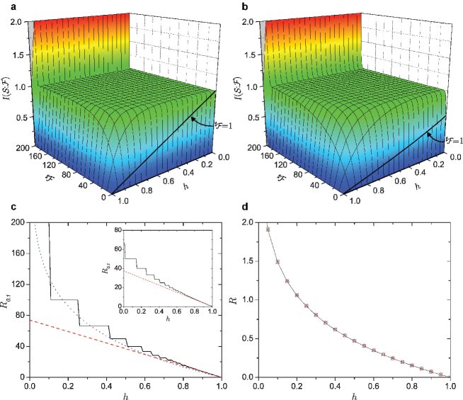
Figure 5: (a,b) Mutual information, $I\left(\mathcal{S}:\mathcal{F}\right)$, versus the fragment size, ${{}^{\sharp}}\mathcal{F}$, and haziness, $h$, of the environment qubits, and (c,d) the redundancy (limiting redundancy), $R_{\delta}$ ($\bar{R}$), versus $h$. The system is initially pure, and $s_{00}=1/2$, $r_{00}=1/2$, and ${{}^{\sharp}}\mathcal{E}=200$. (a,b) Mutual information at $t=\pi/2$ and $t=\pi/4$, respectively. The classical plateau forms in all but the haziest of conditions where the environment is ab initio in a perfect mixture. (c) The redundancy, $R_{\delta}$, at $t=\pi/2$ (and $t=\pi/4$ in the inset). The black line is the exact data. The redundancy initially drops fairly rapidly because of the symmetry of the model but then goes over to a region where it behaves as $1-h$ (shown as the red, dashed line). The blue, dotted curve shows the scaling behavior from Eq. (29), which already reasonably approximates the exact behavior even though ${{}^{\sharp}}\mathcal{F}_{\delta}$ is small. (d) The limiting redundancy, $\bar{R}$, at $t=\pi/2$. There are four different initial states of $\mathcal{S}$: $s_{00}=1/2$ (blue circles), $s_{00}=1/8$ (red crosses), $s_{00}=1/64$ (green squares), and $s_{00}=1/4096$ (magenta triangles). Equation (30) with $R_{\delta}$ from Eq. (29), is plotted (black line) with the exact data for the different initial states of $\mathcal{S}$.

Misaligned $\mathcal{E}$ - As discussed above, a misaligned environment qubit is one that has a larger overlap with an eigenstate of the interaction Hamiltonian, and thus one with a decreased capacity for information. With the interaction Hamiltonian containing $\sigma^{z}$ operators on the environment qubits, the misalignment is the bias in the initial state, Eq. (20), $\sigma=r_{00}-r_{11}$. In Fig. 6(a,b), we show the mutual information versus ${{}^{\sharp}}\mathcal{F}$ and $\sigma$ at $t=\pi/2$ and $t=\pi/4$. The classical plateau is formed for all but the most misaligned states and at the same level, $H_{\mathcal{S}}$. Thus, just as with haziness, misaligned environments also redundantly encode information (i.e., classical information) about $\mathcal{S}$. The redundancy is plotted in Fig. 6(c,d) for these two times. We can see that, for the not too small information deficit $\delta=0.1$, $R_{\delta}$ is initially quite insensitive to the misalignment.

We can get quantitative understanding of how the redundancy behaves if we take $\delta$ to be small. In this case, a large ${{}^{\sharp}}\mathcal{F}_{\delta}$ is necessary to achieve the plateau value of the mutual information within the information deficit $\delta$ and we thus can take all the corresponding decoherence factors $\Lambda_{\mathcal{F}}(t)$, $\Lambda_{\mathcal{E}/\mathcal{F}}(t)$, and $\Lambda_{\mathcal{E}}(t)$ to be very small and expand the entropies in the mutual information, Eq. (48). For pure $\mathcal{E}$, as long as ${{}^{\sharp}}\mathcal{E}\gg{{}^{\sharp}}\mathcal{F}_{\delta}$, this gives the mutual information

$$I\left(\mathcal{S}:\mathcal{F}\right)\approx H_{\mathcal{S}}-\frac{s_{00}s_{11}\ln\frac{s_{00}}{s_{11}}}{\left(s_{00}-s_{11}\right)\ln 2}\left|\Lambda_{\mathcal{F}}(t)\right|^{2}.$$ (31)

Thus, we have

$${{}^{\sharp}}\mathcal{F}_{\delta}\approx\frac{\ln\delta}{\ln\left|\Lambda_{k}\left(t\right)\right|^{2}},$$ (32)

where $\left|\Lambda_{k}\left(t\right)\right|^{2}=\cos^{2}t+\sigma^{2}\sin^{2}t$. Therefore, the redundancy for small information deficit will scale as

$$R_{\delta}\approx\frac{{{}^{\sharp}}\mathcal{E}\ln\left|\Lambda_{k}\left(t\right)\right|^{2}}{\ln\delta}.$$ (33)

This is plotted in Fig. 6(c,d) along with the exact redundancy. Note that, even for the information deficit $\delta=0.1$, the approximate expression is quite good modulo discrete effects. The insets in Fig. 6(c,d) show that as the information deficit is taken to zero, $\delta\to 0$, the scaling predicted for the limiting redundancy, $\bar{R}$ from Eq. (30) with $R_{\delta}$ given by Eq. (33), describes the redundancy behavior of misaligned states very well. At $t=\pi/2$, the redundancy becomes proportional to $\ln\sigma$. Two noticeable features, which are similar to the scaling for hazy, but aligned, environments, given by Eq. (29), are that the redundancy is inversely proportional to the logarithm of the information deficit and that, for small $\delta$, the redundancy is insensitive to the alignment (or initial entropy) of the system. This supports the idea that the redundancy has a universal behavior independent of the system’s initial state.

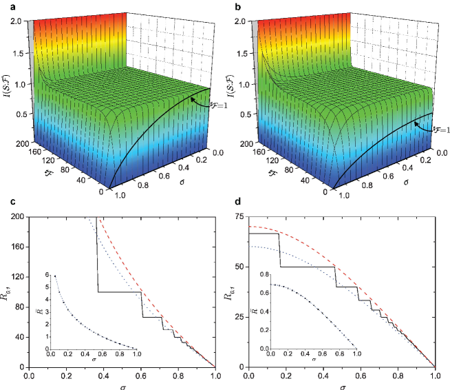
Figure 6: (a,b) Mutual information, $I\left(\mathcal{S}:\mathcal{F}\right)$, versus the fragment size, ${{}^{\sharp}}\mathcal{F}$, and misalignment, $\sigma$, of the environment qubits, and (c,d) the redundancy, $R_{\delta}$, versus $\sigma$. The system and environment are initially pure, and $s_{00}=1/2$ and ${{}^{\sharp}}\mathcal{E}=200$. (a,b) The mutual information at $t=\pi/2$ and $t=\pi/4$, respectively. The classical plateau is formed and is quite large for all but very misaligned states ($\sigma$ near 1). (c,d) The redundancy versus the misalignment at $t=\pi/2$ and $t=\pi/4$, respectively. The black lines are the exact data obtained numerically and the blue dotted line is the scaling given by Eq. (33), which already fits quite well with the numerical results. The red dashed line is the redundancy given by $R_{\delta}\propto\ln\left|\Lambda_{k}\left(t\right)\right|^{2}$ with the constant of proportionality found by retaining all the factors when using Eq. (31). The inserts are the limiting redundancy, $\bar{R}$, given by Eq. (30) (using both the exact data shown as squares and data from Eq. (33) shown as a dashed blue line), which demonstrates that the scaling result is obtained when discrete effects are not present (i.e., in the limit of vanishing information deficit, $\delta\to 0$).

Misaligned and hazy $\mathcal{E}$ - We now consider the case where $\mathcal{E}$ is both misaligned and hazy. In Fig. 7(a,b), the mutual information is plotted versus ${{}^{\sharp}}\mathcal{F}$ and $h/h_{m}$ for $\sigma=0.4$ and $\sigma=0.8$. Just as with misalignment and haziness separately, one still gets the formation of the classical plateau and hence, one still gets redundancy. For fairly hazy environments, the redundancy behaves as for $\sigma=0$ but now with a rescaled haziness $h/h_{m}$. The quantity $h_{m}$ represents the maximum information capacity of a single environment qubit given its alignment with its operator in the Hamiltonian. As before, the redundancy has a linear region where it is proportional to $1-h/h_{m}$. This is shown in Fig. 7(c).

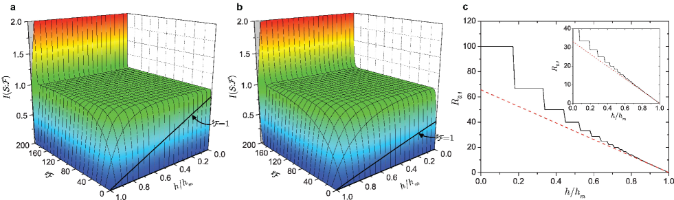
Figure 7: (a,b) Mutual information, $I\left(\mathcal{S}:\mathcal{F}\right)$, versus the fragment size, ${{}^{\sharp}}\mathcal{F}$, and normalized haziness, $h/h_{m}$, of the environment qubits, and (c) the redundancy, $R_{\delta}$, versus $h/h_{m}$. The system is initially pure, and $t=\pi/2$, $s_{00}=1/2$, and ${{}^{\sharp}}\mathcal{E}=200$. (a,b) Mutual information for the misalignments $\sigma=0.4$ ($h_{m}\approx 0.88$) and $\sigma=0.8$ ($h_{m}\approx 0.47$), respectively. The plateau region still forms at the same level, $H_{\mathcal{S}}$, essentially regardless of how hazy or misaligned the environment is initially. (c) Redundancy for $\sigma=0.4$ (the inset is for $\sigma=0.8$). The black line is the exact data and the red dashed line is the linear approximation. As we see, there is still a linear region of the redundancy for fairly hazy environments.

VI Conclusions

We studied how information about a system of interest proliferates throughout an environment under non-ideal initial conditions (namely, hazy or misaligned initial environment states). When a system is undergoing pure decoherence with a set of independent environment components, we showed that, after decoherence has taken place, an environment fragment’s capacity to accept information about a system is given by its ability to increase its entropy. Thus, increasing the overlap of the environment with states that commute with the interaction Hamiltonian (whether by misaligning it or by increasing its haziness) diminishes its ability to increase its entropy and therefore decreases its capacity to accept information about the system. Prior to the onset of good decoherence, complementary information about the system (that is, information about the superposition of pointer states of $\mathcal{S}$) is transferred into the environment, where it is initially spread among many fragments. After the onset of good decoherence, this complementary information is encoded only globally in the environment (i.e., individual fragments do not contain it) . Finally, we examined a model system of a symmetric qubit environment. We found scaling relations that demonstrate a universal behavior of the redundancy (i.e., behavior that is independent of the system’s initial state). Overall, our results show that although non-ideal initial conditions diminish the environment’s capacity to store information, the environment still redundantly obtains information about the system - demonstrating that Quantum Darwinism is robust and non-ideal environments still communicate information redundantly.

Appendix A Qubit interacting with a symmetric environment

The total state of $\mathcal{S}\mathcal{E}$ evolves according to $\rho\left(t\right)=\mathcal{U}\left(t\right)\rho\left(0\right)\mathcal{U}^{\dagger}\left(t\right)$, where $\mathcal{U}\left(t\right)=\exp{\left(-\imath\mathbf{H}_{\mathcal{S}\mathcal{E}}t\right)}$ can be written as

$$\mathcal{U}\left(t\right)=\left|0\right\rangle\left\langle 0\right|\otimes\left[\mathcal{V}\left(t\right)^{\otimes{{}^{\sharp}}\mathcal{E}}\right]+\left|1\right\rangle\left\langle 1\right|\otimes\left[\mathcal{V}\left(-t\right)^{\otimes{{}^{\sharp}}\mathcal{E}}\right].$$ (34)

Here $\mathcal{V}\left(t\right)$ is the unitary matrix $\exp\left[-\imath t\sigma^{z}/2\right].$ The evolution of $\mathcal{S}$ is given by

$$\rho_{\mathcal{S}}(t) = \left(\begin{array}[]{cc}s_{00}&s_{01}\Lambda_{\mathcal{E}}(t)\\ s_{10}\Lambda_{\mathcal{E}}^{\star}(t)&s_{11}\end{array}\right),$$ (37)

with the total decoherence factor

$$\Lambda_{\mathcal{E}}(t)=\prod_{k\in\mathcal{E}}\Lambda_{k}(t)$$ (38)

due to the environment $\mathcal{E}$. Each component of the environment contributes a partial factor

$$\Lambda_{k}\left(t\right)\equiv\mathrm{tr}\left[\bar{\rho}_{r}\left(t\right)\right]=\cos\left(t\right)-\imath\sigma\sin\left(t\right)$$ (39)

to the total decoherence. The state of $\mathcal{S}\mathcal{F}$ is

$$\rho_{\mathcal{S}\mathcal{F}}(t)=\left(\begin{array}[]{cc}s_{00}\tilde{\rho}_{r}\left(t\right)^{\otimes{{}^{\sharp}}\mathcal{F}}&s_{01}\bar{\rho}_{r}\left(t\right)^{\otimes{{}^{\sharp}}\mathcal{F}}\Lambda_{\mathcal{E}/\mathcal{F}}(t)\\ s_{10}\bar{\rho}_{r}^{\dagger}\left(t\right)^{\otimes{{}^{\sharp}}\mathcal{F}}\Lambda_{\mathcal{E}/\mathcal{F}}^{\star}(t)&s_{11}\tilde{\rho}_{r}\left(-t\right)^{\otimes{{}^{\sharp}}\mathcal{F}}\end{array}\right),$$ (40)

where $\tilde{\rho}_{r}\left(t\right)=\mathcal{V}\left(t\right)\rho_{r}\mathcal{V}^{\dagger}\left(t\right)$ is a rotated density matrix on a single environment qubit and $\bar{\rho}_{r}\left(t\right)=\mathcal{V}\left(t\right)\rho_{r}\mathcal{V}\left(t\right)$ is an operator on a single environment qubit.

The von Neumann entropy, $H_{\mathcal{S}}(t)$, can be calculated explicitly by diagonalizing $\rho_{\mathcal{S}}(t)$ to obtain $H_{\mathcal{S}}(t)=H\left(\kappa_{\mathcal{E}}(t)\right)$ with

$$\kappa_{\mathcal{A}}(t)=\frac{1}{2}\left(1+\sqrt{\left(s_{11}-s_{00}\right)^{2}+4\left|s_{01}\right|^{2}\left|\Lambda_{\mathcal{A}}(t)\right|^{2}}\right).$$ (41)

The quantity $\kappa_{\mathcal{A}}(t)$ is one of the eigenvalues of the state of $\mathcal{S}$ when it interacts only with the environment components $k$ for which $k\in\mathcal{A}$. We can likewise readily obtain the entropy of $\mathcal{S}\mathcal{F}$ by utilizing Eq. (5): this entropy is equivalent to the sum of the entropy of the system decohered solely by $\mathcal{E}/\mathcal{F}$, i.e., the remainder of the environment, which is given by $H\left(\kappa_{\mathcal{E}/\mathcal{F}}(t)\right)$, and the entropy of the initial state of the $\mathcal{F}$, $H_{\mathcal{F}}(0)={{}^{\sharp}}\mathcal{F}h$. Thus, the mutual information becomes

$$I\left(\mathcal{S}:\mathcal{F}\right) = \left[H_{\mathcal{F}}\left(t\right)-H_{\mathcal{F}}\left(0\right)\right]$$ (42)

$$+\left[H\left(\kappa_{\mathcal{E}}(t)\right)-H\left(\kappa_{\mathcal{E}/\mathcal{F}}(t)\right)\right].$$

To finish the calculation of the mutual information, we need the remaining term in Eq. (1): the entropy $H_{\mathcal{F}}(t)$. Generally, the calculation of this entropy is difficult, as it requires diagonalizing the reduced density matrix of $\mathcal{F}$, which in this case is

$$\rho_{\mathcal{F}}(t)=s_{00}\tilde{\rho}_{r}\left(t\right)^{\otimes{{}^{\sharp}}\mathcal{F}}+s_{11}\tilde{\rho}_{r}\left(-t\right)^{\otimes{{}^{\sharp}}\mathcal{F}}.$$ (43)

Due the symmetry of the problem, however, Eq. (43) can be diagonalized efficiently numerically using the procedure outlined in Appendix B. Further, in the case of a pure initial environment, one can compute $H_{\mathcal{F}}(t)$ analytically. In the following subsections, we will examine several cases of how the mutual information develops in time for different initial states.

A.1 Pure or mixed $\mathcal{S}$ and pure $\mathcal{E}$

When the environment is pure, the entropy of $\rho_{\mathcal{F}}(t)$ can be found by purifying $\mathcal{S}$ using an ancillary system $\tilde{\mathcal{S}}$ and noting that $H_{\mathcal{F}}(t)=H_{\tilde{\mathcal{S}}\mathcal{S}\mathcal{E}/\mathcal{F}}(t)$. Let $\lambda\equiv\left|s_{01}/\sqrt{s_{00}s_{11}}\right|$ parametrize the existing decoherence of $\mathcal{S}$. Purifying the initial state of $\mathcal{S}$ gives

$$|\psi_{\mathcal{S}\tilde{S}}\rangle=\alpha|00\rangle+\beta|1\tilde{1}\rangle,$$ (44)

where $\left|\alpha\right|^{2}=s_{00}$, $\left|\beta\right|^{2}=s_{11}$, and $|\tilde{1}\rangle=\lambda^{2}|0\rangle+\sqrt{1-\lambda^{2}}|1\rangle$ is a state of $\tilde{\mathcal{S}}$ that would give the existing decoherence of $\mathcal{S}$. To calculate the entropy, $H_{\mathcal{F}}(t)=H_{\tilde{\mathcal{S}}\mathcal{S}\mathcal{E}/\mathcal{F}}(t)$, we can use Eq. (5) with $\mathcal{S}$ replaced by $\mathcal{S}\tilde{\mathcal{S}}$ to show that, in the presence of an initially pure $\mathcal{E}$ (and hence, $\mathcal{E}/\mathcal{F}$), this entropy is equivalent to the entropy of $\mathcal{S}\tilde{\mathcal{S}}$ decohered just by $\mathcal{F}$. The latter is

$$\rho_{\mathcal{S}\tilde{\mathcal{S}}}(t)= s_{00}|00\rangle\langle 00|+\sqrt{s_{00}s_{11}}\Lambda_{\mathcal{F}}(t)|00\rangle\langle 1\tilde{1}|$$ (45)

$$+\sqrt{s_{00}s_{11}}\Lambda_{\mathcal{F}}^{\star}(t)|1\tilde{1}\rangle\langle 00|+s_{11}|1\tilde{1}\rangle\langle 1\tilde{1}|.$$

Since $|00\rangle$ and $|1\tilde{1}\rangle$ are orthogonal, the entropy can be obtained from the eigenvalues of the matrix

$$\left(\begin{array}[]{cc}s_{00}&\sqrt{s_{00}s_{11}}\Lambda_{\mathcal{F}}(t)\\ \sqrt{s_{00}s_{11}}\Lambda_{\mathcal{F}}^{\star}(t)&s_{11}\end{array}\right),$$ (46)

which gives $H\left(\tilde{\kappa}_{\mathcal{F}}(t)\right)$, with

$$\tilde{\kappa}_{\mathcal{A}}(t)=\frac{1}{2}\left(1+\sqrt{\left(s_{11}-s_{00}\right)^{2}+4s_{00}s_{11}\left|\Lambda_{\mathcal{A}}(t)\right|^{2}}\right).$$ (47)

Note that this result, $H_{\mathcal{F}}(t)=H\left(\tilde{\kappa}_{\mathcal{F}}(t)\right)$, is indicating that the entropy of an initially pure $\mathcal{F}$ with time is the same regardless of whether the system was initially pure or mixed. Moreover, as we will see in just a moment, only the discord changes when $\mathcal{S}$ is initially mixed. The mutual information is therefore

$$I\left(\mathcal{S}:\mathcal{F}\right)=H\left(\tilde{\kappa}_{\mathcal{F}}(t)\right)+\left[H\left(\kappa_{\mathcal{E}}(t)\right)-H\left(\kappa_{\mathcal{E}/\mathcal{F}}(t)\right)\right],$$ (48)

where the last two terms in brackets give the quantum discord (and the deviation from good decoherence) for an initially pure $\mathcal{E}$.

As a special case of the above, when $\mathcal{S}$ is pure $\tilde{\kappa}$ reduces to $\kappa$ in Eq. (41) and the mutual information is

$$I\left(\mathcal{S}:\mathcal{F}\right)=H\left(\kappa_{\mathcal{F}}(t)\right)+\left[H\left(\kappa_{\mathcal{E}}(t)\right)-H\left(\kappa_{\mathcal{E}/\mathcal{F}}(t)\right)\right].$$ (49)

This result can be found much more readily by using the equality $H_{\mathcal{F}}(t)=H_{\mathcal{S}\mathcal{E}/\mathcal{F}}(t)$ for bipartite pure states. Then, employing Eq. (7) for $H_{\mathcal{S}\mathcal{E}/\mathcal{F}}(t)$ and $H_{\mathcal{E}/\mathcal{F}}(0)=0$ gives

$$H_{\mathcal{F}}(t)=H_{\mathcal{S}d\mathcal{F}}(t).$$ (50)

Thus we obtain $H_{\mathcal{F}}(t)=H\left(\kappa_{\mathcal{F}}(t)\right)$. This shorter derivation for initially pure $\mathcal{S}$ and $\mathcal{E}$ shows that the entropy of $\mathcal{F}$ is simply the entropy of $\mathcal{S}$ when it is interacting solely with $\mathcal{F}$ Zurek07-1 .

A.2 Pure or mixed $\mathcal{S}$ and hazy $\mathcal{E}$

When the environment is hazy, the entropy of $\rho_{\mathcal{F}}(t)$ can not be found by appealing to entropic properties of bipartite pure states, as was done in the previous section. With our model, however, we can diagonalize $\rho_{\mathcal{F}}(t)$ directly by taking advantage of the symmetry. By using the Wigner D-matrices Cirac99-1 ; Dachsel06-1 ; Miyazaki07-1 , we can rewrite $\rho_{\mathcal{F}}(t)$ into block diagonal form (see Appendix B), with a maximum block dimension equal to $2{{}^{\sharp}}\mathcal{F}+1$. Thus, the complexity for diagonalizing $\rho_{\mathcal{F}}(t)$ is reduced from exponential to polynomial in ${{}^{\sharp}}\mathcal{F}$.

In addition, we can also obtain an analytical result for the entropy when $r_{00}=1/2$ and $t=\pi/2$. Under these two conditions, the reduced density matrix of the environment becomes

$$\rho_{\mathcal{F}}(\pi/2)=s_{00}\left(\begin{array}[]{cc}\frac{1}{2}&-\imath r_{01}\\ \imath r_{10}&\frac{1}{2}\end{array}\right)^{\otimes{{}^{\sharp}}\mathcal{F}}+s_{11}\left(\begin{array}[]{cc}\frac{1}{2}&\imath r_{01}\\ -\imath r_{10}&\frac{1}{2}\end{array}\right)^{\otimes{{}^{\sharp}}\mathcal{F}}$$ (51)

At this time, both terms are diagonal in the same basis . Thus, the matrix can be diagonalized to yield

$$\rho_{\mathcal{F}}(\pi/2)=s_{00}\left(\begin{array}[]{cc}\lambda_{+}&0\\ 0&\lambda_{-}\end{array}\right)^{\otimes{{}^{\sharp}}\mathcal{F}}+s_{11}\left(\begin{array}[]{cc}\lambda_{-}&0\\ 0&\lambda_{+}\end{array}\right)^{\otimes{{}^{\sharp}}\mathcal{F}}$$ (52)

where $\lambda_{\pm}=1/2\pm\left|r_{01}\right|$. Its entropy is then

$$H_{\mathcal{F}}\left(\pi/2\right)=-\sum_{n=0}^{{{}^{\sharp}}\mathcal{F}}\left(\begin{array}[]{c}{{}^{\sharp}}\mathcal{F}\\ n\end{array}\right)\lambda_{\mathcal{F}}\left(n\right)\log_{2}\left[\lambda_{\mathcal{F}}\left(n\right)\right],$$ (53)

where $\lambda_{\mathcal{F}}\left(n\right)=s_{00}\lambda_{-}^{n}\lambda_{+}^{{{}^{\sharp}}\mathcal{F}-n}+s_{11}\lambda_{-}^{{{}^{\sharp}}\mathcal{F}-n}\lambda_{+}^{n}$ are the degenerate eigenvalues of $\rho_{\mathcal{F}}(\pi/2)$. The quantum discord at this time is zero except when ${{}^{\sharp}}\mathcal{F}={{}^{\sharp}}\mathcal{E}$, thus the mutual information is given exactly by Eq. (9) when ${{}^{\sharp}}\mathcal{F}\neq{{}^{\sharp}}\mathcal{E}$. Since $H_{\mathcal{F}}(0)={{}^{\sharp}}\mathcal{F}\,h$, we obtain

$$I\left(\mathcal{S}:\mathcal{F}\right)=H_{\mathcal{F}}\left(\pi/2\right)-{{}^{\sharp}}\mathcal{F}\,h.$$ (54)

In Appendix C we find an asymptotic approximation to Eq. (54).

Appendix B Diagonalizing $\rho_{\mathcal{F}}(t)$

A fragment $\mathcal{F}$ of the environment is described by the density matrix (see Eq. (43))

$$\rho_{\mathcal{F}}(t)=s_{00}\tilde{\rho}_{r}\left(t\right)^{\otimes{{}^{\sharp}}\mathcal{F}}+s_{11}\tilde{\rho}_{r}\left(-t\right)^{\otimes{{}^{\sharp}}\mathcal{F}},$$ (55)

where $\tilde{\rho}_{r}\left(t\right)=\mathcal{V}\left(t\right)\rho_{r}\mathcal{V}^{\dagger}\left(t\right)$ is a rotated density matrix on a single environment qubit and the initial density matrix is given by Eq. (20):

$$\rho_{r}=\left(\begin{array}[]{cc}r_{00}&r_{01}\\ r_{10}&r_{11}\end{array}\right).$$ (56)

To calculate the entropy of $\rho_{\mathcal{F}}(t)$, our strategy is to rewrite the operators of the form $\tilde{\rho}_{r}\left(\pm t\right)^{\otimes{{}^{\sharp}}\mathcal{F}}$ into direct sums of total spin states so that the density matrix becomes block diagonal. Each block can then be diagonalized separately and the computational cost of the computing the entropy is polynomial in ${{}^{\sharp}}\mathcal{F}$ rather than exponential. This process, which consists of three steps, is illustrated in the schematic diagram shown in Fig. 8.

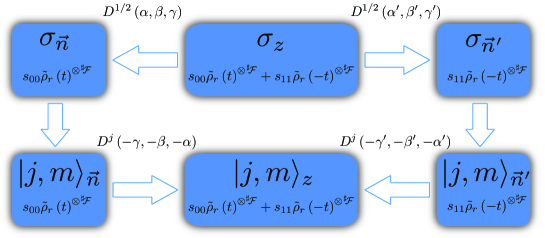
Figure 8: Schematic diagram of the rotating technique used to diagonalize the density matrix $\rho_{\mathcal{F}}(t)$. The density matrix is split into two parts, $s_{00}\tilde{\rho}_{r}\left(t\right)^{\otimes{{}^{\sharp}}\mathcal{F}}$ and $+s_{11}\tilde{\rho}_{r}\left(-t\right)^{\otimes{{}^{\sharp}}\mathcal{F}}$, which are each separately rotated into the basis $\left|j,m\right\rangle_{z}$ by first going through the basis in which the state $\tilde{\rho}_{r}\left(t\right)$ is diagonal.

First, we make a unitary transformation to diagonalize $\tilde{\rho}_{r}\left(t\right)$ and $\tilde{\rho}_{r}\left(-t\right)$. This process can be alternatively understood as a rotating of the density matrix $\tilde{\rho}_{r}\left(t\right)$ with a Wigner D-matrix Cirac99-1 ; Dachsel06-1 ; Miyazaki07-1 , $R(\alpha,\beta,\gamma)$, to change the representation from $\sigma_{z}$ to $\sigma_{\vec{n}}$, where $\vec{n}$ is the Bloch vector of the spin. The second step is to rewrite $\tilde{\rho}_{r}\left(t\right)^{\otimes{{}^{\sharp}}\mathcal{F}}$ into direct sums of total spin states by utilizing the Clebsch-Gordan coefficients. After this step the representation is changed from $\sigma_{\vec{n}}$ to $\left|j,m\right\rangle_{\vec{n}}$. The third step is to rotate from the representation $\left|j,m\right\rangle_{\vec{n}}$ to $\left|j,m\right\rangle_{z}$ by a inverse Wigner D matrix $R(-\gamma,-\beta,-\alpha)\equiv R^{-1}(\alpha,\beta,\gamma)$. We apply the rotating techniques separately to $\tilde{\rho}_{r}\left(t\right)^{\otimes{{}^{\sharp}}\mathcal{F}}$ and $\tilde{\rho}_{r}\left(-t\right)^{\otimes{{}^{\sharp}}\mathcal{F}}$, but finally bring them both into the basis $\left\{\left|j,m\right\rangle_{z}\right\}$ where the blocks are diagonalized.

The details of the procedure start with the rotation by the angles $\alpha$, $\beta$, and $\gamma$:

$$R(\alpha,\beta,\gamma)=e^{-i\alpha J_{z}}e^{-i\beta J_{y}}e^{-i\gamma J_{z}},$$ (57)

where $J_{x}$, $J_{y}$, and $J_{z}$ are the components of the angular momentum (which for our spin system are just the Pauli matrices). The Wigner D matrix is a square matrix of dimension $2j+1$ with general element

$$D_{m,m^{\prime}}^{j} = \left\langle j,m^{\prime}\right|R(\alpha,\beta,\gamma)\left|j,m\right\rangle$$ (58)

$$= e^{-im^{\prime}\alpha}d_{m^{\prime},m}^{j}(\beta)e^{-im\gamma},$$ (59)

where

$$\begin{split}d_{m^{\prime},m}^{j}(\beta)=&\left\langle j,m^{\prime}\right|e^{-i\beta J_{y}}\left|j,m\right\rangle\\ =&[(j+m^{\prime})!(j-m^{\prime})!(j+m)!(j-m)!]^{\frac{1}{2}}\times\sum_{s=\mathrm{max}(0,m-m^{\prime})}^{\mathrm{min}(j+m,j-m^{\prime})}\frac{(-1)^{m^{\prime}-m+s}}{(j+m-s)!s!(m^{\prime}-m+s)!(j-m^{\prime}-s)!}\\ &\times\left(\cos\left[\beta/2\right]\right)^{2j+m-m^{\prime}-2s}\left(\sin\left[\beta/2\right]\right)^{m^{\prime}-m+2s}.\end{split}$$ (60)

The Euler angles $\alpha$, $\beta$, $\gamma$ in the rotation, Eq. (58), are completely determined by the unitary matrix that diagonalizes $\tilde{\rho}_{r}(t)$, $U\tilde{\rho}_{r}(t)U^{\dagger}=\mathrm{Diag}\left[\lambda_{+},\lambda_{-}\right]$, which is

$$U=\left[\begin{array}[]{cc}\frac{-r_{01}e^{-it}}{\sqrt{|r_{01}|^{2}+(r_{00}-\lambda_{+})^{2}}},&\frac{r_{00}-\lambda_{+}}{\sqrt{|r_{01}|^{2}+(r_{00}-\lambda_{+})^{2}}}\\ \frac{r_{11}-\lambda_{-}}{\sqrt{|r_{10}|^{2}+(r_{11}-\lambda_{-})^{2}}},&\frac{-r_{10}e^{it}}{\sqrt{|r_{10}|^{2}+(r_{11}-\lambda_{-})^{2}}}\end{array}\right].$$ (61)

This is equal to the Wigner D matrix

$$D^{1/2}\left(\alpha,\beta,\gamma\right)=\left[\begin{array}[]{cc}e^{-i(\alpha+\gamma)/2}\cos\left(\beta/2\right),&-e^{-i(\alpha-\gamma)/2}\sin\left(\beta/2\right)\\ e^{i(\alpha-\gamma)/2}\sin\left(\beta/2\right),&e^{i(\alpha+\gamma)/2}\cos\left(\beta/2\right).\end{array}\right]$$ (62)

with the Euler angles

$$\alpha=\gamma=t,$$ (63)

$$\sin\left(\beta/2\right)=-\frac{r_{00}-\lambda_{+}}{\sqrt{|r_{01}|^{2}+(r_{00}-\lambda_{+})^{2}}},$$ (64)

and

$$\cos\left(\beta/2\right)=\frac{-r_{01}}{\sqrt{|r_{01}|^{2}+(r_{00}-\lambda_{+})^{2}}}.$$ (65)

The density matrix $\tilde{\rho}_{r}\left(t\right)^{\otimes{{}^{\sharp}}\mathcal{F}}$ becomes

$$\tilde{\rho}_{r}\left(t\right)^{\otimes{{}^{\sharp}}\mathcal{F}}\rightarrow\mathrm{Diag}\left[\lambda_{+},\lambda_{-}\right]^{\otimes{{}^{\sharp}}\mathcal{F}}$$ (66)

and similarly for $\tilde{\rho}_{r}\left(-t\right)^{\otimes{{}^{\sharp}}\mathcal{F}}$.

Utilizing the Clebsch-Gordan coefficients, Eq. (66) can be rewritten as a direct sum of the total spin states,

$$\mathrm{Diag}\left[\lambda_{+},\lambda_{-}\right]^{\otimes{{}^{\sharp}}\mathcal{F}}\rightarrow\oplus_{j=0}^{{{}^{\sharp}}\mathcal{F}/2}\left(M_{j}^{\oplus B_{j}}\right),$$ (67)

where

$$M_{j}=\mathrm{Diag}[\lambda_{+}^{\frac{{{}^{\sharp}}\mathcal{F}}{2}+j}\lambda_{-}^{\frac{{{}^{\sharp}}\mathcal{F}}{2}-j},\lambda_{+}^{\frac{{{}^{\sharp}}\mathcal{F}}{2}+j-1}\lambda_{-}^{\frac{{{}^{\sharp}}\mathcal{F}}{2}-j+1},...,\lambda_{+}^{\frac{{{}^{\sharp}}\mathcal{F}}{2}-j}\lambda_{-}^{\frac{{{}^{\sharp}}\mathcal{F}}{2}+j}]$$ (68)

and

$$B_{j}=\left(\begin{array}[]{c}{{}^{\sharp}}\mathcal{F}\\ {{}^{\sharp}}\mathcal{F}/2-j\end{array}\right)-\left(\begin{array}[]{c}{{}^{\sharp}}\mathcal{F}\\ {{}^{\sharp}}\mathcal{F}/2-j-1\end{array}\right).$$ (69)

The basis of the density matrix $\tilde{\rho}_{r}\left(t\right)^{\otimes{{}^{\sharp}}\mathcal{F}}$ is now $\left\{\left|j,m\right\rangle_{\vec{n}}\right\}$, and under the same procedure the density matrix $\tilde{\rho}_{r}\left(-t\right)^{\otimes{{}^{\sharp}}\mathcal{F}}$ will be in the basis $\left\{\left|j,m\right\rangle_{\vec{n}^{\prime}}\right\}$ with the Bloch vector $\vec{n}^{\prime}$. To get the full density matrix, $\rho_{\mathcal{F}}(t)$, we need to transform them into the same basis $\left\{\left|j,m\right\rangle_{z}\right\}$, which can be done by rotating backwards using $D^{j}(-\gamma,-\beta,-\alpha)$ with the angles corresponding to the forward rotation $D^{1/2}(\alpha,\beta,\gamma)$:

$$\oplus_{j=0}^{{{}^{\sharp}}\mathcal{F}/2}\left(M_{j}^{\oplus B_{j}}\right)\rightarrow\oplus_{j=0}^{{{}^{\sharp}}\mathcal{F}/2}\left[e^{-i(-\gamma)J_{z}}e^{-i(-\beta)J_{y}}e^{-i(-\alpha)J_{z}}M_{j}e^{-i\alpha J_{z}}e^{-i\beta J_{y}}e^{-i\gamma J_{z}}\right]^{\oplus B_{j}}.$$ (70)

Now we can write $\rho_{\mathcal{F}}(t)=s_{00}\tilde{\rho}_{r}\left(t\right)^{\otimes{{}^{\sharp}}\mathcal{F}}+s_{11}\tilde{\rho}_{r}\left(-t\right)^{\otimes{{}^{\sharp}}\mathcal{F}}$ into a block diagonal form in the basis $\left\{\left|j,m\right\rangle_{z}\right\}$, which can be diagonalized efficiently to obtain the entropy of $\mathcal{F}$.

Appendix C Asymptotic approximation

In this appendix, we approximate the expression in Eq. (54) for large ${{}^{\sharp}}\mathcal{F}$. Our starting point is to rewrite Eq. (54) as

$$I\left(\mathcal{S}:\mathcal{F}\right) = H_{\mathcal{S}}-s_{00}\sum_{n=0}^{{{}^{\sharp}}\mathcal{F}}\left(\begin{array}[]{c}{{}^{\sharp}}\mathcal{F}\\ n\end{array}\right)\lambda_{-}^{n}\lambda_{+}^{{{}^{\sharp}}\mathcal{F}-n}\log_{2}\left[1+\frac{s_{11}}{s_{00}}\left(\frac{\lambda_{-}}{\lambda_{+}}\right)^{{{}^{\sharp}}\mathcal{F}-2n}\right]$$

$$-s_{11}\sum_{n=0}^{{{}^{\sharp}}\mathcal{F}}\left(\begin{array}[]{c}{{}^{\sharp}}\mathcal{F}\\ n\end{array}\right)\lambda_{-}^{{{}^{\sharp}}\mathcal{F}-n}\lambda_{+}^{n}\log_{2}\left[1+\frac{s_{00}}{s_{11}}\left(\frac{\lambda_{+}}{\lambda_{-}}\right)^{{{}^{\sharp}}\mathcal{F}-2n}\right]$$

$$\equiv H_{\mathcal{S}}-\Delta I\left(\mathcal{S}:\mathcal{F}\right),$$

where we extracted out the plateau value of the mutual information, $H_{\mathcal{S}}$, and also the initial entropy of $\mathcal{F}$, which cancelled the second term in Eq. (54). The deviation of the mutual information from its plateau value is defined as $\Delta I\left(\mathcal{S}:\mathcal{F}\right)$, which is the term we will approximate. For large ${{}^{\sharp}}\mathcal{F}$, we can use the de Moivre-Laplace theorem to replace the binomial coefficient:

$$2^{{{}^{\sharp}}\mathcal{F}}\left(\begin{array}[]{c}{{}^{\sharp}}\mathcal{F}\\ n\end{array}\right)\left(\frac{1}{2}\right)^{{{}^{\sharp}}\mathcal{F}}\approx\frac{2^{{{}^{\sharp}}\mathcal{F}}}{\sqrt{\pi{{}^{\sharp}}\mathcal{F}/2}}e^{-\left(n-{{}^{\sharp}}\mathcal{F}/2\right)^{2}/\left({{}^{\sharp}}\mathcal{F}/2\right)}.$$ (77)

Performing this replacement and rearranging some terms gives

$$\Delta I\left(\mathcal{S}:\mathcal{F}\right)\approx\frac{\left(2\sqrt{\lambda_{-}\lambda_{+}}\right)^{{{}^{\sharp}}\mathcal{F}}}{\sqrt{\pi{{}^{\sharp}}\mathcal{F}/2}}\sum_{n=0}^{{{}^{\sharp}}\mathcal{F}}e^{-\left(n-{{}^{\sharp}}\mathcal{F}/2\right)^{2}/\left({{}^{\sharp}}\mathcal{F}/2\right)}S\left(n\right),$$ (78)

where

$$S\left(n\right)\equiv s_{00}\left(\frac{\lambda_{-}}{\lambda_{+}}\right)^{n-{{}^{\sharp}}\mathcal{F}/2}\log_{2}\left[1+\frac{s_{11}}{s_{00}}\left(\frac{\lambda_{-}}{\lambda_{+}}\right)^{{{}^{\sharp}}\mathcal{F}-2n}\right]+s_{11}\left(\frac{\lambda_{+}}{\lambda_{-}}\right)^{n-{{}^{\sharp}}\mathcal{F}/2}\log_{2}\left[1+\frac{s_{00}}{s_{11}}\left(\frac{\lambda_{+}}{\lambda_{-}}\right)^{{{}^{\sharp}}\mathcal{F}-2n}\right].$$ (79)

To see how the mutual information approaches the plateau for large ${{}^{\sharp}}\mathcal{F}$, we can make a further approximation by recognizing that the function, $S\left(n\right)$, within the sum peaks at

$$n=\frac{{{}^{\sharp}}\mathcal{F}-\left(\ln\frac{s_{00}}{s_{11}}\right)/\left(\ln\frac{\lambda_{-}}{\lambda_{+}}\right)}{2}$$ (80)

and decays exponentially when away from this maximum at a length scale independent of ${{}^{\sharp}}\mathcal{F}$. When ${{}^{\sharp}}\mathcal{F}$ is large enough, the Gaussian, which has a width proportional to $\sqrt{{{}^{\sharp}}\mathcal{F}}$, is approximately constant where $S\left(n\right)$ is non-negligible. Thus, for large ${{}^{\sharp}}\mathcal{F}$, we approximate the Gaussian as a constant (with its value set at its maximum) and obtain

$$\Delta I\left(\mathcal{S}:\mathcal{F}\right)\approx\frac{\left(2\sqrt{\lambda_{-}\lambda_{+}}\right)^{{{}^{\sharp}}\mathcal{F}}}{\sqrt{\pi{{}^{\sharp}}\mathcal{F}/2}}\sum_{n=0}^{{{}^{\sharp}}\mathcal{F}}S\left(n\right).$$ (81)

This already gives the asymptotic behavior of the mutual information: For large enough ${{}^{\sharp}}\mathcal{F}$, the sum over $S\left(n\right)$ is independent of ${{}^{\sharp}}\mathcal{F}$ because of the exponential decay of $S\left(n\right)$ away from its maximum. However, to remove the sum and obtain a compact expression, we can approximate the sum over $S\left(n\right)$ by an integral. When $\mathcal{E}$ is fairly hazy, $S\left(n\right)$ is smooth as function of $n$ and this approximation is a good one (although, it will have a finite relative error as ${{}^{\sharp}}\mathcal{F}\to\infty$). Changing the sum to an integral and extending the limits to infinity gives the approximate deviation

$$\Delta I\left(\mathcal{S}:\mathcal{F}\right)\approx\Delta I_{app}\left(\mathcal{S}:\mathcal{F}\right)=\frac{\left(2\sqrt{\lambda_{-}\lambda_{+}}\right)^{{{}^{\sharp}}\mathcal{F}}}{\sqrt{\pi{{}^{\sharp}}\mathcal{F}/2}}\int_{-\infty}^{\infty}dnS\left(n\right)=\frac{\left(2\sqrt{\lambda_{-}\lambda_{+}}\right)^{{{}^{\sharp}}\mathcal{F}}}{\sqrt{\pi{{}^{\sharp}}\mathcal{F}/2}}\frac{2\pi\sqrt{s_{00}s_{11}}}{\left(\ln 2\right)\left(\ln\frac{\lambda_{+}}{\lambda_{-}}\right)},$$ (82)

which is the asymptotic approximation used within the paper. In Fig. 9(a) we plot this asymptotic approximation along with the exact data for the deviation of the mutual information from its plateau value. In Fig. 9(b) we plot the relative error

$$\left|\frac{\Delta I_{app}\left(\mathcal{S}:\mathcal{F}\right)-\Delta I\left(\mathcal{S}:\mathcal{F}\right)}{\Delta I\left(\mathcal{S}:\mathcal{F}\right)}\right|.$$ (83)

As can been seen from the figures, the asymptotic approximation correctly describes the decay of the mutual information to its plateau value.

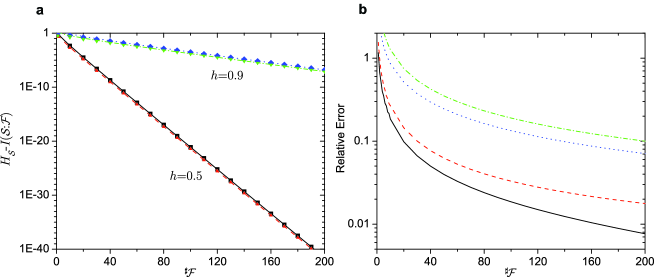
Figure 9: (a) Deviation of the mutual information from its plateau value, $\Delta I\left(\mathcal{S}:\mathcal{F}\right)=H_{\mathcal{S}}-I\left(\mathcal{S}:\mathcal{F}\right)$, versus the fragment size ${{}^{\sharp}}\mathcal{F}$. The exact deviation is plotted for $h=0.5$, $s_{00}=1/2$ (black squares); $h=0.5$, $s_{00}=1/16$ (red triangles); $h=0.9$, $s_{00}=1/2$ (blue diamonds); and $h=0.9$, $s_{00}=1/16$ (green inverse triangles), with the approximate data plotted as a line of the same color as its corresponding exact data. For all but the smallest ${{}^{\sharp}}\mathcal{F}$, the approximation gives the correct decay of the mutual information to its plateau value. Further, changing the value of $H_{\mathcal{S}}$ (by shifting $s_{00}$) does not change the decay behavior to the plateau. (b) Relative error of the asymptotic approximation versus ${{}^{\sharp}}\mathcal{F}$. The errors are for $h=0.5$, $s_{00}=1/2$ (black line); $h=0.5$, $s_{00}=1/16$ (red dashed line); $h=0.9$, $s_{00}=1/2$ (blue dotted line); and $h=0.9$, $s_{00}=1/16$ (green dash-dotted line). The errors decay initially as the approximation of the binomial coefficient by a constant becomes better, but the approximation will contain a finite relative error as ${{}^{\sharp}}\mathcal{F}\to\infty$ due to the approximation of the sum by an integral.

References

- (1) N. Bohr, Nature 121, 580 (1928)
- (2) N. Bohr, Phys. Rev. 48, 696 (1935)
- (3) J. A. Wheeler and W. H. Zurek, Quantum Theory and Measurement (Princeton University Press, Princeton, NJ, 1983)
- (4) W. H. Zurek, Phys. Today 44, 36 (1991)
- (5) W. H. Zurek, Rev. Mod. Phys. 75, 715 (2003)
- (6) E. Joos, H. D. Zeh, C. Kiefer, D. Giulini, J. Kupsch, and I.-O. Stamatescu, Decoherence and the Appearance of a Classical World in Quantum Theory (Springer-Verlag, Berlin, 2003)
- (7) M. Schlosshauer, Decoherence and the Quantum-to-Classical Transition (Springer-Verlag, Berlin, 2008)
- (8) W. H. Zurek, Phys. Rev. D 24, 1516 (1981)
- (9) N. Bohr, in Atomic Physics and Human Knowledge (Wiley, New York, 1958) p. 83
- (10) W. H. Zurek, Phys. Rev. D 26, 1862 (1982); in Quantum Optics, Experimental Gravitation, and Measurement Theory, edited by P. Meystre and M. O. Scully (Plenum Press, New York, 1983) p. 87; See also, arXiv:quant-ph/0111137
- (11) H. Ollivier, D. Poulin, and W. H. Zurek, Phys. Rev. Lett. 93, 220401 (2004); Phys. Rev. A 72, 042113 (2005)
- (12) R. Blume-Kohout and W. H. Zurek, Found. Phys. 35, 1857 (2005); Phys. Rev. A 73, 062310 (2006); Phys. Rev. Lett. 101, 240405 (2008)
- (13) W. H. Zurek, arXiv:0707.2832v1(2007)
- (14) R. Brunner, R. Akis, D. K. Ferry, F. Kuchar, and R. Meisels, Phys. Rev. Lett. 101, 024102 (2008)
- (15) C. H. Bennett, AIP Conf. Proc. 1033, 66 (2008)
- (16) J. P. Paz and A. J. Roncaglia, Phys. Rev. A 80, 042111 (2009)
- (17) M. Zwolak, H. T. Quan, and W. H. Zurek, Phys. Rev. Lett. 103, 110402 (2009)
- (18) W. H. Zurek, Nat. Phys. 5, 181 (2009)
- (19) W. H. Zurek, Ann. Phys.-Leipzig 9, 855 (2000)
- (20) L. Henderson and V. Vedral, J. Phys. A: Math. Gen., 6899(2001)
- (21) H. Ollivier and W. H. Zurek, Phys. Rev. Lett. 88, 017901 (2002)
- (22) T. M. Cover and J. A. Thomas, Elements of information theory (Wiley-Interscience, New York, 2006)
- (23) J. I. Cirac, A. K. Ekert, and C. Macchiavello, Phys. Rev. Lett. 82, 4344 (1999)
- (24) H. Dachsel, J. Chem. Phys. 124, 144115 (2006)
- (25) T. Miyazaki, M. Katori, and N. Konno, Phys. Rev. A 76, 012332 (2007)
- (26) M. Zwolak, J. Chem. Phys. 129, 101101 (2008); Comp. Sci. & Disc. 1, 015002 (2008)