Non-perturbative Green’s functions
and the QCD effective charge

Abstract:

Using as ingredients the non-perturbative solutions of various QCD Green’s function obtained from Schwinger-Dyson equations (SDEs), we study two versions of the QCD effective charge. The first one obtained from the pinch technique gluon self-energy, and the second from the ghost-gluon vertex. Despite the distinct nature of their buildings blocks, the two effectives charges are almost identical in the entire range of momenta, due to a fundamental identity relating the ghost dressing function with the two form factors of Green’s function, which is of central importance in the PT-BFM formalism. In this talk, we outline how to derive this crucial identity from the SDEs of the aforementioned Green’s functions. The renormalization procedure that preserves the validity of this identity is discussed in detail. Most importantly, we show that due to the infrared finiteness of the gluon propagator, the QCD charge obtained with either definition freezes in the deep infrared, in agreement with theoretical and phenomenological expectations.

1 Introduction

One of the most difficult problems in QCD is to understand the interface between the perturbative and non-perturbative regimes. Both sophisticated theoretical tools [1, 2] as well as more phenomenologically oriented approaches [3] indicate that this connection is not abrupt, but rather smooth.

Without any doubt, a continuous interpolation between the perturbative and the non-perturbative region is intimately related to the behavior of the QCD fundamental coupling [4]. However, we know by now, that the smoothness in this transition can not be achieved with perturbative assumption of a coupling with singular growth (Landau pole) in the infrared. Indeed, all accumulated evidence points toward the need of a freezing of the QCD effective charge at small momenta [1, 2, 3], where $\alpha(q^{2})$ develops an infrared fixed point and QCD has a conformal window at low energy [5].

The infrared finiteness of the effective charge can be considered as one of the manifestation of the phenomenon of dynamical gluon mass generation [1, 6] revealing in this way, its profound connection with the most fundamental Green’s functions of QCD, such as the gluon and ghost propagators [4]. Indeed, the basic ingredients that enter in its definition must contain the right information and be combined in a very precise way in order to endow the effective charge with the required physical and field-theoretic properties [2].

In this talk, we will show how different QCD Green’s functions can be combined in order to form renormalization group (RG) invariant quantities which eventually may be associated to a definition of an effective charge [4]. Specifically, we will consider firstly the effective charge obtained within the pinch technique (PT) framework [1, 7], and its correspondence [8] with the background-field method (BFM) [9]. The PT effective charge constitutes the most direct non-abelian generalization of the familiar concept of the QED effective charge. The second definition involves the ghost and gluon self-energies [10], in the Landau gauge, and in the kinematic configuration where the well-known Taylor non-renormalization theorem [11] becomes applicable.

2 Definitions and ingredients

Let us introduce some of the basic ingredients necessary for the definition of the two effective charges we want to study. In the Landau gauge, the full gluon propagator $\Delta_{\mu\nu}(q)$ is transverse, and omiting the color indices, its general form is given by

$$\Delta_{\mu\nu}(q)=-iP_{\mu\nu}(q)\Delta(q^{2}),\quad\mbox{with}\quad P_{\mu\nu}(q)=g_{\mu\nu}-\frac{q_{\mu}q_{\nu}}{q^{2}}\,,$$ (1)

where the scalar function $\Delta(q^{2})$ is related to the all order self-energy $\Pi_{\mu\nu}(q)=P_{\mu\nu}(q)\Pi(q^{2})$ through $\Delta^{-1}(q^{2})=q^{2}+i\Pi(q^{2})$. The full ghost propagator $D(q^{2})$ and its dressing function $F(q^{2})$ are related by

$$D(q^{2})=\frac{iF(q^{2})}{q^{2}}.$$ (2)

In our construction, a special role is played by the auxiliary two-point function $\Lambda_{\mu\nu}(q)$, represented in Fig. 1 and defined as [12]

$$\Lambda_{\mu\nu}(q)=g_{\mu\nu}G(q^{2})+\frac{q_{\mu}q_{\nu}}{q^{2}}L(q^{2}) = -ig^{2}C_{A}\int_{k}H^{(0)}_{\mu\rho}D(k+q)\Delta^{\rho\sigma}(k)\,H_{\sigma\nu}(k,q),$$ (3)

where $C_{\rm{A}}$ is the Casimir eigenvalue of the adjoint representation [ $\,C_{\rm{A}}\,=\,N$ for $SU(N)$ ], and $\int_{k}\equiv\mu^{2\varepsilon}(2\pi)^{-d}\int\!d^{d}k$, with $d=4-\epsilon$ the dimension of space-time. The vertex $H_{\mu\nu}(k,q)$ is also represented in Fig. 1, and its tree-level counterpart is given $H_{\mu\nu}^{(0)}=ig_{\mu\nu}$. An additional constraint on the behavior $H_{\mu\nu}(k,q)$ is imposed by the WI (Ward identity)

$$q^{\nu}H_{\mu\nu}(k,q)=-i\bm{\Gamma}_{\mu}(k,q)\,,$$ (4)

where $\bm{\Gamma}_{\mu}(k,q)$ is the all-order ghost vertex, with $k$ representing the momentum of the gluon and $q$ the one of the anti-ghost; at tree-level $\bm{\Gamma}^{(0)}_{\mu}(k,q)=-q_{\mu}$.

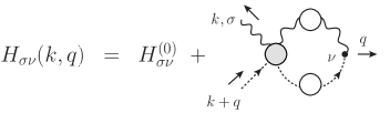
Figure 1: Diagrammatic representation of $H$.

2.1 The pinch technique effective charge

The heart of the PT effective charge definition lies on the construction of a new effective gluon propagator, $\widehat{\Delta}(q^{2})$, which captures the running of the QCD $\beta$ function, exactly as happens with the vacuum polarization in the case of QED [2, 7, 8]. Already at one-loop level, the PT gluon propagator displays the desired coefficient in front of the perturbative logarithm, namely

$$\widehat{\Delta}^{-1}(q^{2})=q^{2}\left[1+bg^{2}\ln\left(\frac{q^{2}}{\mu^{2}}\right)\right],$$ (5)

where $b=11C_{A}/48\pi^{2}$ is the first coefficient of the QCD $\beta$-function when the number of fermions $n_{f}=0$ (quarkless QCD).

In addition, to all order $\widehat{\Delta}^{-1}(q^{2})$ is universal (i.e. process-independent), and therefore it does not depend on the details of the process where it is embedded as shown in Fig. 2.

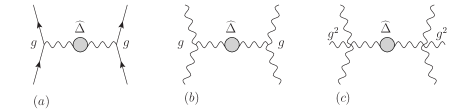
Figure 2: The universal PT coupling.

One important point, explained in detail in the literature, is the (all-order) correspondence between the PT and the Feynman gauge of the BFM [8, 9]. In fact, one can generalize the PT construction [8] in such a way as to reach diagrammatically any value of the gauge fixing parameter of the BFM, and in particular the Landau gauge. In what follows we will implicitly assume the aforementioned generalization of the PT, given that the main identity we will use to relate the two effective charges is valid only in the Landau gauge.

Due to the Abelian WIs satisfied by the PT- BFM Green’s functions, the renormalization constants of the gauge-coupling and of the PT gluon self-energy, defined as

$$g(\mu^{2})=Z_{g}^{-1}(\mu^{2})g_{0}\,;\qquad\widehat{\Delta}(q^{2},\mu^{2})=\widehat{Z}^{-1}_{A}(\mu^{2})\widehat{\Delta}_{0}(q^{2}),$$ (6)

where the “0” subscript indicates bare quantities, satisfy the QED-like relation

$${Z}_{g}={\widehat{Z}}^{-1/2}_{A}.$$ (7)

Thus, it follows immediately that the product

$${\widehat{d}}_{0}(q^{2})=g^{2}_{0}\widehat{\Delta}_{0}(q^{2})=g^{2}(\mu^{2})\widehat{\Delta}(q^{2},\mu^{2})={\widehat{d}}(q^{2}),$$ (8)

retains the same form before and after renormalization, i.e., it forms a RG-invariant ($\mu$-independent) quantity [1, 2, 8]. For asymptotically large momenta one may extract from ${\widehat{d}}(q^{2})$ a dimensionless quantity by writing,

$${\widehat{d}}(q^{2})=\frac{\overline{g}^{2}(q^{2})}{q^{2}},$$ (9)

where $\overline{g}^{2}(q^{2})$ is the RG-invariant effective charge of QCD; at one-loop (use Eq. (5) into (8))

$$\overline{g}^{2}(q^{2})=\frac{g^{2}}{1+bg^{2}\ln\left(q^{2}/\mu^{2}\right)}=\frac{1}{b\ln\left(q^{2}/\Lambda^{2}_{\mathrm{QCD}}\right)}\,,$$ (10)

where $\Lambda_{\mathrm{QCD}}$ denotes an RG-invariant mass scale of a few hundred ${\rm MeV}$.

Being a direct consequence of the WIs satisfied by the PT Green’s function, Eq. (8) may be employed either perturbatively or non-perturbatively, provided that one has information on the IR behavior of the PT-BFM gluon propagator $\widehat{\Delta}(q^{2})$.

However, thanks to a general relation connecting the PT-BFM $\widehat{\Delta}(q^{2})$ and the conventional gluon propagator $\Delta(q^{2})$, all the non-perturbative information we have gathered about $\Delta(q^{2})$ may also be used. Specifically, the aforementioned formal all-order relation states that [13]

$$\Delta(q^{2})=\left[1+G(q^{2})\right]^{2}\widehat{\Delta}(q^{2}),$$ (11)

where $G(q^{2})$ is the form factor of the $g_{\mu\nu}$ component appearing on the definition of $\Lambda^{\mu\nu}$ given in Eq.(3). Note that, due to its BRST origin, the above relation must be preserved after renormalization. Specifically, denoting by $Z_{\Lambda}$ the renormalization constant relating the bare and renormalized functions, $\Lambda_{0}^{\mu\nu}$ and $\Lambda^{\mu\nu}$, through

$$g^{\mu\nu}+\Lambda^{\mu\nu}(q,\mu^{2})=Z_{\Lambda}(\mu^{2})[g^{\mu\nu}+\Lambda_{0}^{\mu\nu}(q)],$$ (12)

then from (7) and (11) follows the additional relation

$$Z_{g}^{-1}=Z_{A}^{1/2}Z_{\Lambda},$$ (13)

which it will be useful in the following subsection.

At lowest order, it is straightforward to verify, that the role of the function the $1+G(q^{2})$, obtained from Eq. (3), is to restore the $\beta$ function coefficient in front of UV logarithm. Explicitly, we have at one-loop (in the Landau gauge) [12]

$$1+G(q^{2})=1+\frac{9}{4}\frac{C_{\rm{A}}g^{2}}{48\pi^{2}}\ln\left(\frac{q^{2}}{\mu^{2}}\right)\;\qquad\Delta^{-1}(q^{2}) = q^{2}\left[1+\frac{13}{2}\frac{C_{\rm{A}}g^{2}}{48\pi^{2}}\ln\left(\frac{q^{2}}{\mu^{2}}\right)\right].$$ (14)

Using Eq. (11) we therefore recover the $\widehat{\Delta}^{-1}(q^{2})$ of Eq. (5), as we should.

Then, non-perturbatively, one substitutes into Eq. (11) the $1+G(q^{2})$ and $\Delta(q^{2})$ obtained from either the lattice or SD analysis, to obtain $\widehat{\Delta}(q^{2})$. As explained above, the combination formed by

$$\widehat{d}(q^{2})=\frac{g^{2}\Delta(q^{2})}{\left[1+G(q^{2})\right]^{2}}\,,$$ (15)

is independent of the renormalization point $\mu$ i.e. a RG-invariant quantity.

2.2 Gluon-ghost vertex

Another possibility for defining the QCD effective charge can be obtained starting from the various QCD vertices. The basic idea behind is to recognize the RG-invariant quantities we may form out of these vertices. The downside of this construction lies in the fact that it involves all the momentum scales present in the vertex in question, and further assumptions about their kinematic configuration need to be introduced, in order to express the charge as a function of a single variable. The ghost-gluon vertex has been particularly popular in this context, especially in conjunction with Taylor’s non-renormalization theorem and the corresponding kinematics [10].

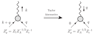
Figure 3: The ghost-gluon vertex and the Taylor kinematics.

For the case of the ghost-gluon vertex (see Fig. 3), the renormalization constants involved are

$$\Delta(q^{2},\mu^{2})=Z^{-1}_{A}(\mu^{2})\Delta_{0}(q^{2}), F(q^{2},\mu^{2})=Z^{-1}_{c}(\mu^{2})F_{0}(q^{2}),$$

$$\bm{\Gamma}^{\nu}(k,q,\mu^{2})=Z_{1}(\mu^{2})\bm{\Gamma}^{\nu}_{0}(k,q), g_{0}=Z_{g^{\prime}}(\mu^{2})g^{\prime}.$$ (16)

Notice that a priori $Z_{g^{\prime}}$ defined as $Z_{g^{\prime}}=Z_{1}Z_{A}^{-1/2}Z_{c}^{-1}$, does not have to coincide with the $Z_{g}$ appearing in (6); however, as we will see in the next section, they do coincide by virtue of the basic identity we will derive there.

Choosing the special Taylor’s kinematic configuration, where the incoming ghost has a vanishing momentum (i.e. $k_{\mu}\to-q_{\mu}$), one may impose the following additional condition one the renormalization constant $Z_{1}$ (valid only in the Landau gauge), namely $Z_{1}=Z_{g^{\prime}}Z_{A}^{1/2}Z_{c}=1$, from which follows immediately that

$$Z_{g^{\prime}}^{-1}=Z_{A}^{1/2}Z_{c}.$$ (17)

Thus, the product

$$\widehat{r}(q^{2})={g^{\prime}}^{2}\Delta(q^{2};\mu^{2})F^{2}(q^{2};\mu^{2})={g^{\prime}}_{0}^{2}\Delta_{0}(q^{2})F^{2}_{0}(q^{2}),$$ (18)

forms a dimensionful $\mu$-independent combination. Therefore, for asymptotically large $q^{2}$, in analogy to Eq. (9), one can define an alternative QCD running coupling as

$$\widehat{r}(q^{2})=\frac{\overline{g}_{\mathrm{gh}}^{2}(q^{2})}{q^{2}}.$$ (19)

Using then Eq. (14), and the fact that

$$F^{-1}(q^{2})=1+\frac{9}{4}\frac{C_{\rm{A}}g^{2}}{48\pi}\ln\left(\frac{q^{2}}{\mu^{2}}\right),$$ (20)

it is straightforward to verify that $\overline{g}_{\mathrm{gh}}^{2}(q^{2})$ and $\overline{g}^{2}(q^{2})$ display the same one-loop behavior, since, perturbatively the function $1+G(q^{2})$ is the inverse of the ghost dressing function $F(q^{2})$. As we will see in the next section, this is nothing more than the one-loop manifestation of the more general identity relating $G(q^{2})$ and $F(q^{2})$.

3 A special relation between Green’s functions

In this section, we sketch the main steps needed to derive the central identity, valid only in the Landau gauge, relating the ghost dressing function with a particular combination of the form-factors $G(q^{2})$ and $L(q^{2})$ appearing in the tensorial decomposition of $\Lambda_{\mu\nu}$ given in Eq. (3).

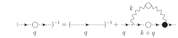
Figure 4: The SDE for the ghost.

First, consider the standard SD equation for the ghost propagator (Fig 4),

$$iD^{-1}(q^{2})=q^{2}+ig^{2}C_{\rm{A}}\int_{k}\Gamma^{\mu}\Delta_{\mu\nu}(k)\bm{\Gamma}^{\nu}(k,q)D(k+q).$$ (21)

Then, contract both sides of the defining equation (3) by the combination $q^{\mu}q^{\nu}$ to get

$$[G(q^{2})+L(q^{2})]q^{2}=g^{2}C_{\rm{A}}\int_{k}q_{\rho}\Delta^{\rho\sigma}(k)\,q^{\nu}H_{\sigma\nu}(k,q)D(k+q).$$ (22)

Using Eq. (4) and the transversality of the full gluon propagator, we can see that the rhs of Eq. (22) is precisely the integral appearing in the ghost SDE (21). Therefore

$$[G(q^{2})+L(q^{2})]q^{2}=iD^{-1}(q^{2})-q^{2},$$ (23)

or, in terms of the ghost dressing function $F(q^{2})$ [viz. Eq. (2)]

$$\boxed{1+G(q^{2})+L(q^{2})=F^{-1}(q^{2})}$$ (24)

The above relation, derived here from the SD equations of the theory, has been first obtained in [14], in the framework of the Batalin-Vilkovisky quantization formalism. As was shown there, the relation is a direct consequence of the fundamental BRST symmetry.

Now, let us construct the dynamical equations governing the behavior of the functions $G(q^{2})$ and $L(q^{2})$. The tensorial projection of both functions in terms of $\Lambda_{\mu\nu}$ may be obtained from Eq. (3), where in $d$ dimensions, we have

$$G(q^{2})=\frac{1}{(d-1)q^{2}}\left(q^{2}\Lambda_{\mu}^{\mu}-q^{\mu}q^{\nu}\Lambda_{\mu\nu}\right),\qquad L(q^{2})=\frac{1}{(d-1)q^{2}}\left(dq^{\mu}q^{\nu}\Lambda_{\mu\nu}-q^{2}\Lambda_{\mu}^{\mu}\right),$$ (25)

which then gives, in terms of the SDE integrals

$$G(q^{2}) = \frac{g^{2}C_{\rm{A}}}{d-1}\left[\int_{k}\Delta^{\rho\sigma}(k)\,H_{\sigma\rho}(k,q)D(k+q)+i\frac{1}{q^{2}}\int_{k}q^{\rho}\Delta_{\rho\sigma}(k)\,{\bm{\Gamma}}^{\sigma}(k,q)D(k+q)\right],$$

$$L(q^{2}) = -\frac{g^{2}C_{\rm{A}}}{d-1}\left[i\frac{d}{q^{2}}\int_{k}q^{\rho}\Delta_{\rho\sigma}(k)\,{\bm{\Gamma}}^{\sigma}(k,q)D(k+q)\!+\!\!\int_{k}\Delta^{\rho\sigma}(k)\,H_{\sigma\rho}(k,q)D(k+q)\right]\!.$$ (26)

In this point some words about the renormalization and approximations we will employ in Eq. (26) are in order. Let us start with the renormalization procedure. As mentioned before, since the origin of (24) is the BRST symmetry, it should not be deformed after renormalization. Combining the definitions of (12) and (16), we see that in order to preserve the relation (24) we must impose that $Z_{\Lambda}=Z_{c}$. In addition, by virtue of (4), and for the same reason, we have that, in the Landau gauge, ${\bm{\Gamma}}_{\nu}(k,q)$ and $H_{\sigma\nu}(k,q)$ must be renormalized by the same renormalization constant, namely $Z_{1}$ [viz. Eq. (16)]; for the Taylor kinematics, we have that $Z_{1}=1$.

Then, approximating the two vertices, $H_{\mu\nu}(k,q)=ig_{\mu\nu}$, and $\bm{\Gamma}_{\mu}(k,q)=-q_{\mu}$, by their tree-level values, then, setting $f(k,q)\equiv(k\cdot q)^{2}/{k^{2}q^{2}}$, one may show that [4]

$$F^{-1}(q^{2}) = Z_{c}+g^{2}C_{\rm{A}}\int_{k}[1-f(k,q)]\Delta(k)D(k+q),$$

$$1+G(q^{2}) = Z_{c}+\frac{g^{2}C_{\rm{A}}}{d-1}\int_{k}[(d-2)+f(k,q)]\Delta(k)D(k+q),$$

$$L(q^{2}) = \frac{g^{2}C_{\rm{A}}}{d-1}\int_{k}[1-d\,f(k,q)]\Delta(k)D(k+q)\,,$$ (27)

which clearly satisfies Eq. (24).

We next go to the Euclidean space, by setting $-q^{2}=q^{2}_{\mathrm{E}}$, and defining $\Delta_{\mathrm{E}}(q^{2}_{\mathrm{E}})=-\Delta(-q^{2}_{\mathrm{E}})$, $D_{\mathrm{E}}(q^{2}_{\mathrm{E}})=-D(-q^{2}_{\mathrm{E}})$, and for the integration measure $\int_{k}=i\int_{k_{\mathrm{E}}}$. Then, suppressing the subscript “E” and setting $q^{2}=x$, $k^{2}=y$, we have that $k\cdot q=\sqrt{xy}\cos\theta$, and so $(k\cdot q)^{2}/q^{2}=y\cos^{2}\theta$, and $(k+q)^{2}=x+y+2\sqrt{xy}\cos\theta$, we arrive at (see details in [4])

$$1+G(x) = Z_{c}-\frac{\alpha_{s}C_{\rm{A}}}{16\pi}\left[\frac{F(x)}{x}\int_{0}^{x}\!\!\!dy\ y\left(3+\frac{y}{3x}\right)\Delta(y)+\int_{x}^{\infty}\!\!\!dy\left(3+\frac{x}{3y}\right)\Delta(y)F(y)\right],$$

$$L(x) = \frac{\alpha_{s}C_{\rm{A}}}{12\pi}\left[\frac{F(x)}{x^{2}}\int_{0}^{x}\!\!\!dy\ y^{2}\Delta(y)+x\int_{x}^{\infty}\!\!\!dy\frac{\Delta(y)F(y)}{y}\right],$$

$$F^{-1}(x) = Z_{c}-\frac{\alpha_{s}C_{\rm{A}}}{16\pi}\left[\frac{F(x)}{x}\int_{0}^{x}\!\!\!dy\ y\left(3-\frac{y}{x}\right)\Delta(y)+\int_{x}^{\infty}\!\!\!dy\left(3-\frac{x}{y}\right)\Delta(y)F(y)\right].$$ (28)

Then, it is easy to see (e.g., by means of the change of variables $y=zx$) that if $\Delta$ and $F$ are IR finite, Eq. (28) yields the important result $L(0)=0$ [4]. Let us now assume that the renormalization condition for $F(x)$ was chosen to be $F(\mu^{2})=1$. This condition, when inserted into the third equation of (28), allows one to express $Z_{c}$ as

$$Z_{c}=1+\frac{\alpha_{s}C_{\rm{A}}}{16\pi}\left[\frac{1}{\mu^{2}}\int_{0}^{\mu^{2}}\!\!\!dyy\left(3-\frac{y}{\mu^{2}}\right)\Delta(y)+\int_{\mu^{2}}^{\infty}\!\!\!dy\left(3-\frac{\mu^{2}}{y}\right)\Delta(y)F(y)\right],$$ (29)

and may be used to cast (28) into a manifestly renormalized form. Note that if one choses $F(\mu^{2})=1$, then one cannot choose simultaneously $G(\mu^{2})=0$, because that would violate the identity of Eq. (24), given that $L(\mu^{2})\neq 0$. In fact, once $F(\mu^{2})=1$ has been imposed, the value of $G(\mu^{2})$ is completely determined from its own equation, i.e. the first equation in (28).

In addition, in the MOM scheme $\Delta(q^{2})$ and $\widehat{\Delta}(q^{2})$ cannot be made equal at the renormalization point, since Eq. (11) implies $\widehat{\Delta}^{(-1)}(\mu^{2})=\mu^{2}\left[1+G^{2}(\mu^{2})\right]^{2}$.

Now, let us to return to the couplings, and discuss the implications of the identity given by Eq. (24). First of all, comparing Eq. (13) and Eq. (17), it is clear that $g(\mu)=g^{\prime}(\mu)$, by virtue of $Z_{\Lambda}=Z_{c}$. Therefore, using Eq. (11), and the definitions given in Eqs. (8) and (18), one can obtain a relation between the two RG-invariant quantities, $\widehat{r}(q^{2})$ and $\widehat{d}(q^{2})$, namely

$$\widehat{r}(q^{2})=[1+G(q^{2})]^{2}F^{2}(q^{2})\widehat{d}(q^{2}).$$ (30)

From this last equality, follows that $\alpha_{{\scriptscriptstyle\mathrm{PT}}}(q^{2})$ and $\alpha_{\mathrm{gh}}(q^{2})$ are related by

$$\alpha_{\mathrm{gh}}(q^{2})=[1+G(q^{2})]^{2}F^{2}(q^{2})\alpha_{{\scriptscriptstyle\mathrm{PT}}}(q^{2}),$$ (31)

After using Eq. (24), we have that

$$\alpha_{{\scriptscriptstyle\mathrm{PT}}}(q^{2})=\alpha_{\mathrm{gh}}(q^{2})\left[1+\frac{L(q^{2})}{1+G(q^{2})}\right]^{2}\,.$$ (32)

Evidently, the two couplings can only coincide at two points: (i) at $q^{2}=0$, where, due to the fact that $L(0)=0$ , we have that $\alpha_{\mathrm{gh}}(0)=\alpha_{{\scriptscriptstyle\mathrm{PT}}}(0)$, and (ii) at $q^{2}=\infty$, given that in the deep UV $L(q^{2})$ approaches a constant. Note in fact that the two effective charges cannot coincide at the renormalization point $\mu$, where $\alpha_{\mathrm{gh}}(\mu^{2})=[1-L(\mu^{2})]^{2}\alpha_{{\scriptscriptstyle\mathrm{PT}}}(\mu^{2})$; this can be understood also in terms of the discussion following Eq. (29).

4 Schwinger-Dyson input and numerical analysis

Now we are in the position to compute the QCD effective charges defined above, using as input the non-perturbative solutions of SDE for the various Green’s functions appearing in their definitions. More specifically, we will solve numerically a system of three coupled non-linear integral equations in the Landau gauge, containing $\Delta(q^{2})$, $F(q^{2})$, and $G(q^{2})$ as unknown quantities.

Once solutions for these three functions have been obtained, then $L(q^{2})$ is fully determined by its corresponding equation, namely the second one in Eq. (28).

Figure 5: The new SDE for the gluon one-loop dressed diagrams.

The two SD equations determining $F(q^{2})$, $G(q^{2})$ are given in Eq. (28). The SD equation governing $\Delta(q^{2})$, is given by [12]

$$[1+G(q^{2})]^{2}\Delta^{-1}(q^{2})P_{\mu\nu}(q)=q^{2}P_{\mu\nu}(q)+i\sum_{i=1}^{4}(a_{i})_{\mu\nu},$$ (33)

where the diagrams $(a_{i})_{\mu\nu}$ are shown in Fig. 5. As explained in [12], due to the abelian WI satisfied by the fully-dressed vertices in the PT-BFM scheme, we have that $q^{\mu}[(a_{1})_{\mu\nu}+(a_{2})_{\mu\nu}]=q^{\mu}[(a_{3})_{\mu\nu}+(a_{4})_{\mu\nu}]=0$. This last property enforces the the transversality of the gluon self-energy “order-by-order” in the dressed-loop expansion, which is one of the central features of the gauge-invariant SD truncation scheme defined within the PT-BFM framework.

After introducing appropriate Ansätze for the aforementioned fully-dressed vertices, we finally arrive at the integral equation

$$[1+G(q^{2})]^{2}\Delta^{-1}(q^{2})\, = \,q^{2}-\frac{g^{2}C_{A}}{6}\left[\int_{k}\!\!\Delta(k)\Delta(k+q)f_{1}+\int_{k}\!\!\Delta(k)f_{2}-\frac{1}{2}\int_{k}\frac{q^{2}}{k^{2}(k+q)^{2}}\right]$$ (34)

$$+ g^{2}C_{A}\bigg{[}\frac{4}{3}\int_{k}\left[k^{2}-\frac{(k\cdot q)^{2}}{q^{2}}\right]D(k)D(k+q)-2\int_{k}D(k)\bigg{]}\,,$$

with

$$f_{1} = 20q^{2}+18k^{2}-6(k+q)^{2}+\frac{(q^{2})^{2}}{(k+q)^{2}}-(k\cdot q)^{2}\bigg{[}\frac{20}{k^{2}}+\frac{10}{q^{2}}+\frac{q^{2}}{k^{2}(k+q)^{2}}+\frac{2(k+q)^{2}}{q^{2}k^{2}}\bigg{]}\,,$$

$$f_{2} = -\frac{27}{2}-8\frac{k^{2}}{(k+q)^{2}}+8\frac{q^{2}}{(k+q)^{2}}+4\frac{(k\cdot q)^{2}}{k^{2}(k+q)^{2}}-4\frac{(k\cdot q)^{2}}{q^{2}(k+q)^{2}}\,,\$$ (35)

The important point is that, by virtue of the poles introduced into the equation through the particular Ansätze employed [1, 12, 15], one obtains an IR finite solution for the gluon propagator, i.e.a solution with $\Delta^{-1}(0)>0$, in complete agreement with a large body of lattice data [16].

In Figs. 6 we show the results for $\Delta(q^{2})$ and $F(q^{2})$ renormalized at three different points, $\mu=\{4.3,10,22\}$ GeV with $\alpha(\mu^{2})=\{0.21,0.16,0.13\}$ respectively. On the right panel we plot the corresponding $F(q^{2})$ renormalized at the same points. Notice that the solutions obtained are in qualitative agreement with recent results from large-volume lattices [16] where the both quantities, $\Delta(q^{2})$ and $F(q^{2})$, reach finite (non-vanishing) values in the deep IR.

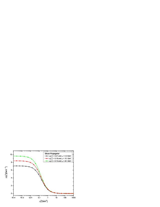
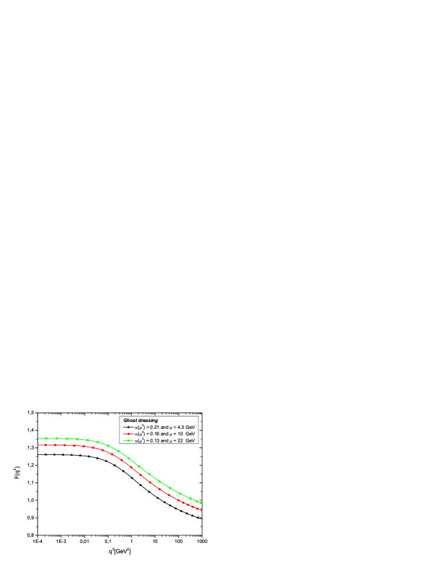
Figure 6: Left panel: Numerical solutions for the gluon propagator obtained from the SDE renormalized at three different points, $\mu=\{4.3,10,22\}$ GeV with $\alpha(\mu^{2})=\{0.21,0.16,0.13\}$. Right panel: The ghost dressing function $F(q^{2})$ obtained from its corresponding SDE and renormalized at the same points.

The results for $1+G(q^{2})$ and $L(q^{2})$, renormalized at the same points, are presented in Fig. 7. As we can see, the function $1+G(q^{2})$ is also IR finite exhibiting a plateau for values of $q^{2}<0.1\mbox{GeV}^{2}$. In the UV region, we instead recover the perturbative behavior (14). On the other hand, $L(q^{2})$ shows a maximum in the intermediate momentum region, while, as expected, $L(0)=0$.

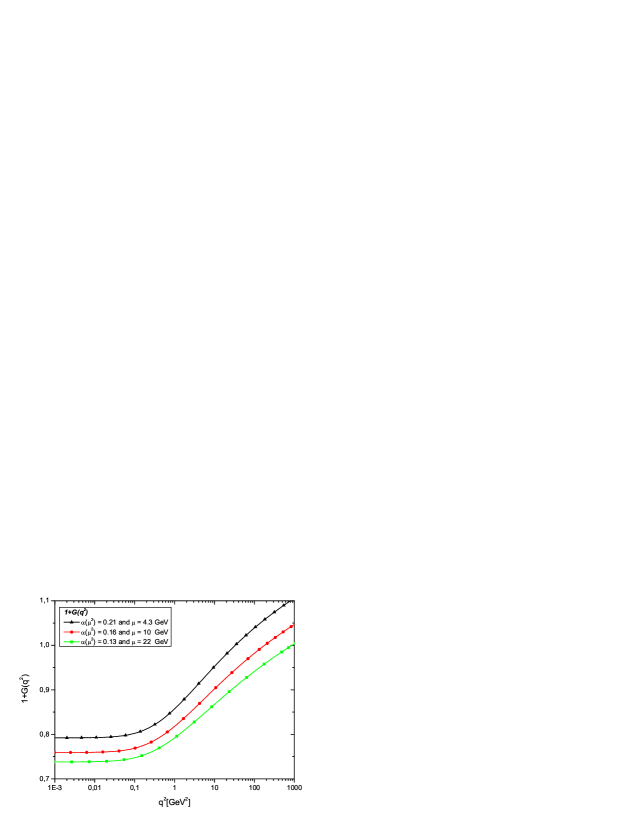
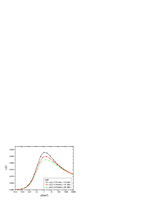
Figure 7: Left panel: $1+G(q^{2})$ determined from Eq. (3.8), using the solutions for $\Delta(q^{2})$ and $D(q^{2})$ presented in the Fig. 6 at the same renormalization points. Right panel: The function $L(q^{2})$ obtained from Eq. (3.8).

With all ingredients defined, the first thing one can check is that indeed Eq. (15) gives rise to a RG-invariant combination. Using the latter definition, we can combine the different data sets for $\Delta(q^{2})$ and $[1+G(q^{2})]^{2}$ at different renormalization points, to arrive at the curves shown on the left panel of Fig. 8. Indeed, we see that all curves, for different values of $\mu$, merge one into the other proving that the combination $\widehat{d}(q^{2})$ is independent of the renormalization point chosen.

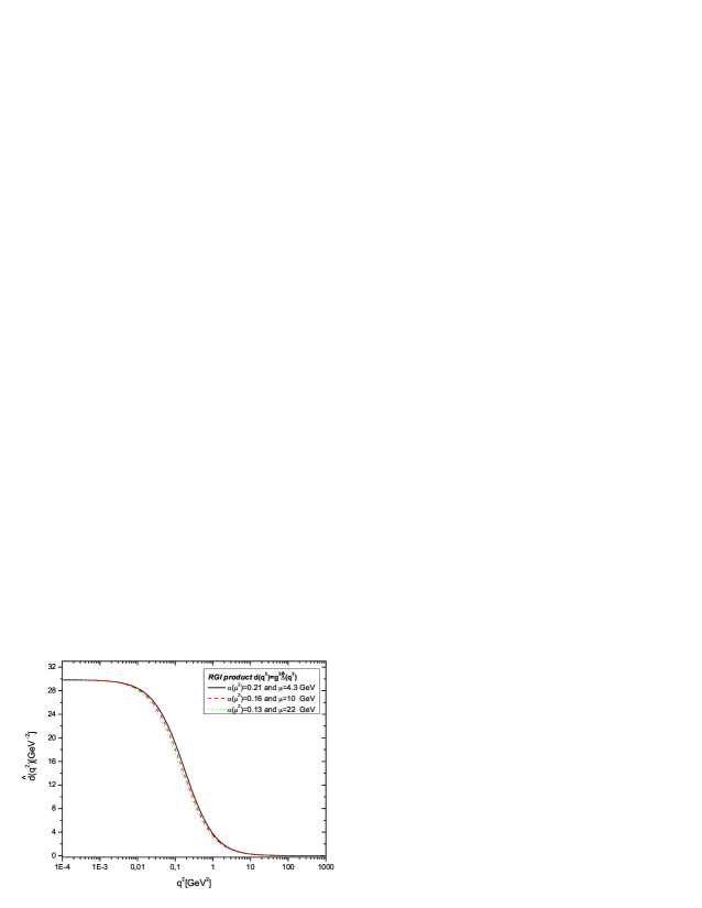
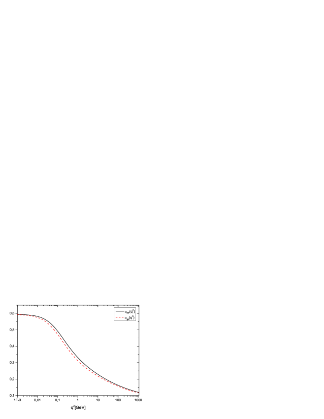
Figure 8: Left panel: The $\widehat{d}(q^{2})$ obtained by combining $\Delta(q^{2})$ and $[1+G(q^{2})]^{2}$ according to Eq. (2.15). Right panel: $\alpha_{\mathrm{gh}}(q^{2})$ vs $\alpha_{\mathrm{PT}}(q^{2})$, for $m_{0}=500\,\mbox{MeV}$.

From the dimensionful ${\widehat{d}}(q^{2})$ we must now extract a dimensionless factor, ${\overline{g}}^{2}(q^{2})$, corresponding to the running coupling (effective charge). Given that $\Delta(q^{2})$ is IR finite, the physically meaningful procedure is to factor out from ${\widehat{d}}(q^{2})$ a massive propagator $[q^{2}+m^{2}(q^{2})]^{-1}$,

$$\widehat{d}(q^{2})=\frac{\overline{g}^{2}(q^{2})}{q^{2}+m^{2}(q^{2})}\,,$$ (36)

where for the mass we will assume “power-law” running [17], $m^{2}(q^{2})=m^{4}_{0}/(q^{2}+m^{2}_{0})$.

Thus, it follows from Eq. (36), that the effective charge $\alpha_{{\scriptscriptstyle\mathrm{PT}}}(q^{2})=\overline{g}^{2}(q^{2})/4\pi$ is identified as being

$$4\pi\alpha_{{\scriptscriptstyle\mathrm{PT}}}(q^{2})=[q^{2}+m^{2}(q^{2})]\widehat{d}(q^{2})\,.$$ (37)

Finally we compare numerically the two effective charges, $\alpha_{{\scriptscriptstyle\mathrm{PT}}}(q^{2})$ and $\alpha_{\mathrm{gh}}(q^{2})$ on the right panel of Fig. 8. First, we determine $\alpha_{{\scriptscriptstyle\mathrm{PT}}}(q^{2})$ obtained using (37), then we obtain $\alpha_{\mathrm{gh}}(q^{2})$ with help of (32) and the results for $1+G(q^{2})$ and $L(q^{2})$ shown in Fig. 7. As we can clearly see, both couplings freeze at the same finite value, exhibiting a plateau for values of $q^{2}<0.02\,\mbox{GeV}^{2}$, while in the UV both show the expected perturbative behavior. They differ only slightly in the intermediate region where the values of $L(q^{2})$ are appreciable.

5 Conclusions

In this talk we have compared the definition of two QCD effective charges, $\alpha_{\scriptscriptstyle{\mathrm{PT}}}(q^{2})$ and $\alpha_{\mathrm{gh}}(q^{2})$, obtained within two vastly different frameworks: the PT-BFM on the one hand, and the ghost-gluon vertex (with the Taylor-kinematics) on the other.

Despite their distinct field-theoretic origin, their dynamics involves the gluon propagator $\Delta(q^{2})$ as a common ingredient and two different ingredients, which participate in a non-trivial identity. This identity, which is valid only in the Landau gauge, relates the ghost dressing function, $F(q^{2})$, with the two form-factors, $G(q^{2})$ and $L(q^{2})$.

As consequence of the aforementioned identity, we have shown that the two effective charges are almost identical in the entire range of physical momenta. More specifically, they coincide exactly in the deep infrared, where they freeze at a common finite value, signaling the appearance of IR fixed point and a conformal window in QCD [5], in agreement with a variety of phenomenological studies [18].

- [1] J. M. Cornwall, Phys. Rev. D 26, 1453 (1982); J. M. Cornwall and J. Papavassiliou, Phys. Rev. D 40, 3474 (1989).
- [2] D. Binosi and J. Papavassiliou, Nucl. Phys. Proc. Suppl. 121, 281 (2003); A. C. Aguilar and J. Papavassiliou, JHEP 0612, 012 (2006); A. C. Aguilar and J. Papavassiliou, arXiv:0910.4142 [hep-ph].
- [3] A. C. Mattingly and P. M. Stevenson, Phys. Rev. D 49, 437 (1994); Y. L. Dokshitzer, G. Marchesini and B. R. Webber, Nucl. Phys. B 469 (1996) 93; A. M. Badalian and V. L. Morgunov, Phys. Rev. D 60, 116008 (1999); S. J. Brodsky, S. Menke, C. Merino and J. Rathsman, Phys. Rev. D 67, 055008 (2003); G. Grunberg, Phys. Rev. D 29, 2315 (1984); Phys. Rev. D 73, 091901 (2006); A. A. Natale, arXiv:0910.5689 [hep-ph].
- [4] A. C. Aguilar, D. Binosi, J. Papavassiliou and J. Rodriguez-Quintero, Phys. Rev. D 80, 085018 (2009).
- [5] S. J. Brodsky and G. F. de Teramond, Phys. Lett. B 582, 211 (2004).
- [6] A. C. Aguilar, A. A. Natale and P. S. Rodrigues da Silva, Phys. Rev. Lett. 90, 152001 (2003).
- [7] N. J. Watson, Nucl. Phys. B 494, 388 (1997).
- [8] D. Binosi and J. Papavassiliou, Phys. Rev. D 66(R), 111901 (2002); A. Pilaftsis, Nucl. Phys. B 487, 467 (1997); D. Binosi and J. Papavassiliou, Phys. Rept. 479, 1 (2009).
- [9] L. F. Abbott, Nucl. Phys. B 185, 189 (1981).
- [10] R. Alkofer, C. S. Fischer and F. J. Llanes-Estrada, Phys. Lett. B 611, 279 (2005).
- [11] J. C. Taylor, Nucl. Phys. B 33, 436 (1971); W. J. Marciano and H. Pagels, Phys. Rept. 36, 137 (1978).
- [12] A. C. Aguilar, D. Binosi and J. Papavassiliou, Phys. Rev. D 78, 025010 (2008).
- [13] P. A. Grassi, T. Hurth and M. Steinhauser, Annals Phys. 288, 197 (2001); D. Binosi and J. Papavassiliou, Phys. Rev. D 66(R), 025024 (2002).
- [14] T. Kugo, arXiv:hep-th/9511033; P. A. Grassi, T. Hurth and A. Quadri, Phys. Rev. D 70, 105014 (2004).
- [15] R. Jackiw and K. Johnson, Phys. Rev. D 8, 2386 (1973); J. M. Cornwall and R. E. Norton, Phys. Rev. D 8 (1973) 3338; E. Eichten and F. Feinberg, Phys. Rev. D 10, 3254 (1974).
- [16] A. Cucchieri and T. Mendes, PoS LAT2007, 297 (2007); I. L. Bogolubsky, E. M. Ilgenfritz, M. Muller-Preussker and A. Sternbeck, PoS LAT2007, 290 (2007); T. Iritani, H. Suganuma and H. Iida, arXiv:0908.1311 [hep-lat].
- [17] M. Lavelle, Phys. Rev. D 44, 26 (1991); A. C. Aguilar and J. Papavassiliou, Eur. Phys. J. A 35, 189 (2008); D. Dudal et al., Phys. Rev. D 78, 065047 (2008).
- [18] F. Halzen, G. I. Krein and A. A. Natale, Phys. Rev. D 47, 295 (1993); A. C. Aguilar, A. Mihara and A. A. Natale, Phys. Rev. D 65, 054011 (2002); Int. J. Mod. Phys. A 19, 249 (2004).