Effect of electron-lattice interaction on the phase separation in strongly correlated electron systems with two types of charge carriers

Abstract

The effect of electron-lattice interaction is studied for a strongly correlated electron system described by the two-band Hubbard model. A two-fold effect of electron-lattice interaction is taken into account: in non-diagonal terms, it changes the effective bandwidth, whereas in diagonal terms, it shifts the positions of the bands and the chemical potential. It is shown that this interaction significantly affects the doping range corresponding to the electronic phase separation and can even lead to a jump-like transition between states with different values of strains.

I Introduction

A typical feature of the strongly correlated electron systems is the formation of inhomogeneous states dagbook ; dagsci . The nature of such inhomogeneities based on the electron correlations. However, their specific manifestations can include the effects of different degrees of freedom existing in the solids: spin, charge, orbital, and lattice khom . A strong electron-lattice coupling plays a fundamental role in such actively studied systems as high-temperature superconductors, manganites, cobaltites, and other related materials egami1 ; egami2 . An important characteristics of all these materials is a complicated electronic structure involving two or more conduction bands. The simplest model allowing appropriate description of electron correlation effects is Hubbard model and its multiband generalization pwand ; varma ; wagner .

In Ref. tb1, it was demonstrated that existence of two bands in the Hubbard model gives rise to the existence of the electronic phase separation even in the absence of any type of additional factors (spin, charge, orbital, etc.). However, these factors are necessary to give a realistic description of the particular physical systems. For example, taking into account spin and orbital variables allows a detailed picture of the phase diagram for manganites tb2 ; tb3 . Including in the model the possibility of the spin-state transitions gives an explanation of the phase separation in cobaltites ooco ; ishih . An important and vast field of research is a problem of existence of inhomogeneities in high-temperature superconductors, especially in cuprates egami2 . In this field, the multiband Hubbard model provides some insight in the properties of the cuprate superconductors.

Electron-lattice coupling was incorporated in the multiband Hubbard model to describe electronic structure of cuprates and manganites lor ; poliak ; suph ; indusi . In these papers, the main emphasis was put on the polaron effects or the influence of the electron-phonon interaction on electron pairing. Here we use a similar type of the electron-lattice coupling to analyze its effect on the formation of the inhomogeneous states within two-band Hubbard model.

II Model and a qualitative analysis

Let us consider a strongly correlated electron system with two types of charge carriers, $a$ and $b$, interacting with lattice strains $u$ (static dispersionless phonons). Here, we limit ourselves to the case of small strains, $|u|\ll 1$, when the theory of elasticity is applicable.

The Hamiltonian of such a system can be written as

$$H=H_{el}+H_{U}+H_{el-ph}+H_{ph}.$$ (1)

Here, $H_{el}$ corresponds to the energy of charge carries without taking into account the interaction between them

$$H_{el}=-\sum_{\langle\mathbf{i}\mathbf{j}\rangle,\sigma}\left(t^{a}a^{\dagger}_{\mathbf{i}\sigma}a_{\mathbf{j}\sigma}+t^{b}b^{\dagger}_{\mathbf{i}\sigma}b_{\mathbf{j}\sigma}\right)-\Delta E\sum_{\mathbf{i}\sigma}n_{\mathbf{i},\sigma}^{b},$$ (2)

where $a^{\dagger}_{\mathbf{i}\sigma}$ and $a_{\mathbf{i}\sigma}$ ($b^{\dagger}_{\mathbf{i}\sigma}$ and $b_{\mathbf{i}\sigma}$) are the creation and annihilation operators for $a$ ($b$) electrons at site $\mathbf{i}$ with spin projection $\sigma$, $\langle...\rangle$ means the summation over the nearest neighbors, $t^{a}$ and $t^{b}$ are the corresponding hopping integrals, $\Delta E$ is the energy shift between $a$ and $b$ bands, and $n^{a}_{\mathbf{i}\sigma}=a^{\dagger}_{\mathbf{i}\sigma}a_{\mathbf{i}\sigma}$ and $n^{b}_{\mathbf{i}\sigma}=b^{\dagger}_{\mathbf{i}\sigma}b_{\mathbf{i}\sigma}$ are the number operators for $a$ and $b$ electrons, respectively.

The $H_{U}$ term corresponding to the on-site Coulomb repulsion of charge carriers has the form

$$H_{U}\!=\!\frac{1}{2}\!\sum_{\mathbf{i},\sigma}\left(U_{a}n^{a}_{\mathbf{i}\sigma}n^{a}_{\mathbf{i}\bar{\sigma}}\!+\!U_{b}n^{b}_{\mathbf{i}\sigma}n^{b}_{\mathbf{i}\bar{\sigma}}\right)\!+\!\frac{U_{ab}}{2}\!\sum_{\mathbf{i},\sigma,\sigma^{\prime}}n^{a}_{\mathbf{i}\sigma}n^{b}_{\mathbf{i}\sigma^{\prime}},$$ (3)

where $U_{a}$, $U_{a}$, and $U_{ab}$ are the energies of Coulomb repulsion between two $a$, two $b$, and one $a$ and one $b$ electrons at one lattice site, respectively, and $\bar{\sigma}$ means the spin projection with the sign opposite to that of $\sigma$. We assume that the on-site Coulomb repulsion is large, $U_{a},U_{b},U_{ab}\gg zt$ ($z$ is the number of nearest-neighbor sites, $z=6$ for the simple cubic lattice considered in this paper) and $U_{a}\sim U_{b}\sim U_{ab}\sim U$.

The electron-lattice interaction can be chosen in the following form

$$H_{el-ph}=\sum_{\langle\mathbf{i}\mathbf{j}\rangle,\sigma}\left(\lambda\,a^{\dagger}_{\mathbf{i}\sigma}a_{\mathbf{j}\sigma}u_{\mathbf{j}}+\lambda^{\prime}b^{\dagger}_{\mathbf{i}\sigma}b_{\mathbf{j}\sigma}u_{\mathbf{j}}\right)$$ (4)

$$+\sum_{\mathbf{i},\sigma}\left(\lambda_{a}u_{\mathbf{i}}n^{a}_{\mathbf{i}\sigma}+\lambda_{b}u_{\mathbf{i}}n^{b}_{\mathbf{i}\sigma}\right),$$ (5)

where $\lambda$, $\lambda^{\prime}$ and $\lambda_{a,b}$ are corresponding constants of the electron-phonon interaction and $u_{\mathbf{i}}$ are the local distortions corresponding to site $\mathbf{i}$. Thus, we take into account the effect of lattice strains both on the on-site electron energy and intersite charge transfer.

We approximate the phonon self-energy term $H_{ph}$ as an elastic energy of the system depending on distortions at different sites

$${\cal{F}}_{\rm elast}=\frac{K}{2}\sum_{\mathbf{i}}u^{2}_{\mathbf{i}},$$ (6)

where $K$ is the elastic modulus.

We analyze the problem in adiabatic approximation considering phonons as a classical static elastic field. To find a self-consistent solution to the problem, we first perform averaging of the Hamiltonian over the electronic degrees of freedom. From the condition of the energy minimum with respect to strains, $\partial{\langle H(u_{\mathbf{i}})\rangle}/\partial u_{\mathbf{i}}=0$, we obtain

$$\bar{u}_{\mathbf{i}}=-\frac{\lambda z\langle a^{\dagger}_{\mathbf{i}\sigma}a_{\mathbf{j}\sigma}\rangle+\lambda^{\prime}z\langle b^{\dagger}_{\mathbf{i}\sigma}b_{\mathbf{j}\sigma}\rangle+\lambda_{a}\langle n_{\mathbf{i}}^{a}\rangle+\lambda_{b}\langle n_{\mathbf{i}}^{b}\rangle}{K},$$ (7)

where $\mathbf{i}$ and $\mathbf{j}$ are the nearest-neighbor sites.

Using Eq. (7), we can present the effective electron Hamiltonian as

$$H_{\rm eff} = -\sum_{\langle\mathbf{i}\mathbf{j}\rangle,\sigma}\left[\left(t^{a}-\lambda\bar{u}_{\mathbf{i}}\right)a^{\dagger}_{\mathbf{i}\sigma}a_{\mathbf{j}\sigma}+\left(t^{b}-\lambda^{\prime}\bar{u}_{\mathbf{i}}\right)b^{\dagger}_{\mathbf{i}\sigma}b_{\mathbf{j}\sigma}\right]$$ (8)

$$- \sum_{\mathbf{i}\sigma}\left[\Delta E+(\lambda_{a}-\lambda_{b})\bar{u}_{\mathbf{i}}\right]n_{\mathbf{i},\sigma}^{b}+H_{U}$$

$$- \sum_{\mathbf{i},\sigma}(\mu-\lambda_{a}\bar{u}_{\mathbf{i}})\left(n^{a}_{\mathbf{i}\sigma}+n^{b}_{\mathbf{i}\sigma}\right)+\frac{K}{2}\sum_{\mathbf{i}}\bar{u}^{2}_{\mathbf{i}},$$

here $\mu$ is the chemical potential.

Hamiltonian Eq. (8) clearly demonstrates that the effect of electron-lattice interaction is two-fold. This interaction in non-diagonal terms changes the effective bandwidth whereas in diagonal terms, it shifts the positions of the bands and the chemical potential. In the earlier analysis tb1 ; bianc , we have shown that the qualitative features of the phase diagram for the two-band Hubbard model are mainly determined by two dimensionless parameters: the ratio of the bandwidths and the relative positions of the bands. Thus, to construct a minimal model capturing the main physical effects of electron-lattice interaction, it is sufficient to keep only $\lambda$ and $\lambda_{b}$. In addition, we put $\Delta E=0$ to emphasize the effect of band shift related only to the electron-lattice interaction. As a result, we get

$$\bar{u}_{\mathbf{i}}=-\frac{\lambda z\langle a^{\dagger}_{\mathbf{i}\sigma}a_{\mathbf{j}\sigma}\rangle+\lambda_{b}\langle n_{\mathbf{i}}^{b}\rangle}{K}$$ (9)

and

$$H_{\rm eff}=-\sum_{\langle\mathbf{i}\mathbf{j}\rangle,\sigma}\left[\left(t^{a}-\lambda\bar{u}_{\mathbf{i}}\right)a^{\dagger}_{\mathbf{i}\sigma}a_{\mathbf{j}\sigma}+t^{b}b^{\dagger}_{\mathbf{i}\sigma}b_{\mathbf{j}\sigma}\right]+H_{U}$$

$$+\sum_{\mathbf{i}\sigma}\lambda_{b}\bar{u}_{\mathbf{i}}n_{\mathbf{i},\sigma}^{b}-\sum_{\mathbf{i},\sigma}\mu\left(n^{a}_{\mathbf{i}\sigma}+n^{b}_{\mathbf{i}\sigma}\right)+\frac{K}{2}\sum_{\mathbf{i}}\bar{u}^{2}_{\mathbf{i}}.\,\,$$ (10)

Starting from Hamiltonian (II), we can point out the main qualitative effects of the electron-lattice interaction in the two-band model. In the absence of doping, $n=0$, bands $a$ and $b$ are empty and their centers coincide. With the growth of $n$ the wider band $a$ begins to be filled up from the bottom. The band filling is accompanied by strain $\bar{u}_{\mathbf{i}}=-\lambda z\langle a^{\dagger}_{\mathbf{i}\sigma}a_{\mathbf{j}\sigma}\rangle/K$. The average $\langle a^{\dagger}_{\mathbf{i}\sigma}a_{\mathbf{j}\sigma}\rangle$ is proportional to the hopping probability and thus is positive. The strain $\bar{u}_{\mathbf{i}}$ is positive if $\lambda<0$ and negative if $\lambda>0$. From Eq. (II), it is easy to see that at any sign of $\lambda$ the bandwidth increases with the strain. At a certain doping level, the chemical potential attains the bottom of the narrower band $b$ and this second band starts to be filled up. In this range of doping, we have two types of the electrons and the energy of the system depends on $n$ in a rather complicated manner due to electron-electron correlations. As we have shown earlier tb1 , such situation is favorable for the phase separation even in the absence of the electron-lattice interaction.

However, the characteristic feature of the system under study is the dependence of the effective band shift $\Delta E_{\rm eff}=-\lambda_{b}\bar{u}_{\mathbf{i}}$ on the strain and, hence, on the doping, according to Eq. (9). The sign of the shift depends on the signs of $\lambda$ and $\lambda_{b}$. A simple analysis of Eqs. (9) and (II) shows that for the same signs of $\lambda$ and $\lambda_{b}$ the value of $\Delta E_{\rm eff}$ is negative and the sign of $\bar{u}_{\mathbf{i}}$ remains the same at any $n$. If the signs of $\lambda$ and $\lambda_{b}$ are different, the strain can change its sign at some doping level. The change of the sign of the strain results in the change of the sign of the effective band shift $\Delta E_{\rm eff}$.

The dependence of $\Delta E_{\rm eff}$ on doping can give rise to a more sophisticated behavior of the system. If at some doping level $n^{*}$, the narrower band crosses the bottom of the wider band, that is $\lambda_{b}^{2}n^{*}/K\gtrsim zt_{a}$, then it could be favorable to have almost all electrons in the $b$ band. So, there appears a competition between two states with different values of the strain. It suggests the possibility of a transition between these two states, which can have a jump-like form.

In the next section, we present a quantitative analysis of the possible situations.

III Mean field approach

In the limit of strong electron correlations, $U\rightarrow\infty$, we can describe the evolution of the band structure with the change of $n$ following the method presented in Ref. tb1, . We introduce one-particle Green functions for $a$ and $b$ electrons. For band $a$, we have

$$G_{a\sigma}(\mathbf{i}-\mathbf{j},\,t)=-i\langle\hat{T}a_{\mathbf{i}\sigma}(t)a^{{\dagger}}_{\mathbf{j}\sigma}(0)\rangle,$$ (11)

where $\hat{T}$ is the time-ordering operator. The similar expression can be written for band $b$. The equation of motion for the one-particle Green function with Hamiltonian (II) includes two-particle Green functions of the form

$${\cal{G}}_{a\sigma,b\sigma^{\prime}}(\mathbf{i}-\mathbf{j},\,t)=-i\langle\hat{T}a_{\mathbf{i}\sigma}(t)n^{b}_{\mathbf{i}\sigma^{\prime}}(t)a^{{\dagger}}_{\mathbf{j}\sigma}(0)\rangle\,.$$ (12)

In the considered limit of strong on-site Coulomb repulsion, the presence of two electrons at the same site is unfavorable, and the two-particle Green function is of the order of $1/U$. The equation of motion for two-particle Green functions includes the three-particle terms coming from the commutator of $a_{\mathbf{i}\sigma}(t)$ or $b_{\mathbf{i}\sigma}(t)$ with the $U$ terms of Hamiltonian (II), which are of the order of $1/U^{2}$ and so on. In these equations, following the Hubbard I approach Hub , we neglect the terms of the order of $1/U^{2}$ and use the following decoupling in the Green functions $\langle\hat{T}a_{\mathbf{i}+\mathbf{m}\sigma}(t)n^{b}_{\mathbf{i}\sigma^{\prime}}(t)a^{{\dagger}}_{\mathbf{j}\sigma}(0)\rangle\to\langle n^{b}_{\mathbf{i}\sigma^{\prime}}\rangle\langle\hat{T}a_{\mathbf{i}+\mathbf{m}\sigma}(t)a^{{\dagger}}_{\mathbf{j}\sigma}(0)\rangle$. As a result, we derive a closed system for the one- and two-particle Green functions tb1 ; Hub . This system can be solved in a conventional manner by passing from the time-space $(t,\mathbf{r})$ to the frequency-momentum $(\omega,\mathbf{k})$ representation. We limit ourselves to consideration of the case when the total number of electrons per site does not exceed unity, $n=n^{a}+n^{b}\leq 1$. The upper Hubbard sub-bands are empty, and we can proceed to the limit $U\rightarrow\infty$. In this case, the one-particle Green functions are independent of $U$ and can be written in the frequency-momentum representation as tb1

$$G_{a\sigma}(\mathbf{k},\omega) = \frac{g_{a\sigma}}{\omega+\mu-g_{a\sigma}w_{a}(1-\lambda\bar{u}/t_{a})\zeta(\mathbf{k})}\,,$$

$$G_{b\sigma}(\mathbf{k},\omega) = \frac{g_{b\sigma}}{\omega+\mu-\lambda_{b}\bar{u}-g_{b\sigma}w_{b}\zeta(\mathbf{k})}\,,$$ (13)

where we put $\bar{u}_{\mathbf{i}}=\bar{u}$ assuming a homogeneous strain and introduce the following notation $w_{\alpha}=zt_{\alpha}$, $\alpha=a$ or $b$,

$$g_{\alpha\sigma}=1-\sum_{\sigma^{\prime}}n^{\bar{\alpha}}_{\sigma^{\prime}}-n^{\alpha}_{\bar{\sigma}}\,,$$ (14)

$n^{\alpha}_{\sigma}=\langle n^{\alpha}_{\mathbf{i}\sigma}\rangle$ is the average number of electrons per site in state $(\alpha,\sigma)$, and $\zeta(\mathbf{k})$ is the spectral function depending on the lattice symmetry. In the considered case of the simple cubic lattice, $\zeta({\bf k})=-\left[\cos(k^{1}d)+\cos(k^{2}d)+\cos(k^{3}d)\right]/3$, $d$ is the lattice constant. In the main approximation in $1/U$, the magnetic ordering does not appear and we can assume that $n^{\alpha}_{\uparrow}=n^{\alpha}_{\downarrow}\equiv n^{\alpha}/2$. Below we omit spin indices.

IV Results and discussion

Equations (III) and (14) demonstrate that the filling of the bands depends on the strain $\bar{u}$ and the number of electrons in one band depends on that in another band. Using the expression for the density of states $\rho_{\alpha}(E)=-\pi^{-1}\textmd{Im}\int G_{\alpha}(\mathbf{k},E+i0)d^{3}{\bf k}/(2\pi)^{3}$, we get expressions for the numbers of electrons in bands $a$ and $b$

$$n^{a}\!=\!2g_{a}n_{0}\!\!\left[\frac{\mu}{g_{a}w_{a}\!\left(1\!-\!\lambda\bar{u}/t_{a}\right)}\right]\!\!,\,n^{b}\!=\!2g_{b}n_{0}\!\!\left[\!\frac{\mu\!-\!\lambda_{b}\bar{u}}{g_{b}w_{b}}\!\right]$$ (15)

where

$$n_{0}(\mu^{\prime})=\int\limits_{-1}^{\mu^{\prime}}dE^{\prime}\,\rho_{0}(E^{\prime})\,,$$ (16)

and $\rho_{0}(E^{\prime})=\displaystyle\int d^{3}\mathbf{k}\,\delta(E^{\prime}-\zeta(\mathbf{k}))/(2\pi)^{3}$ is the density of states for free electrons (with the energy normalized by unity, $|E|\leq 1$). The chemical potential $\mu$ in Eq. (15) can be found from the equality

$$n=n^{a}(\mu)+n^{b}(\mu).$$ (17)

Equations (15) include average strain $\bar{u}$, which itself depends on $n^{b}$ and an average $\langle a^{\dagger}_{\mathbf{i}\sigma}a_{\mathbf{j}\sigma}\rangle$. The latter can be expressed in terms of the Green function as

$$\langle a^{\dagger}_{\mathbf{i}\sigma}a_{\mathbf{j}\sigma}\rangle = -iG_{a\sigma}(\mathbf{i}-\mathbf{j},-0)$$

$$= -i\int\frac{d\omega d^{3}\mathbf{k}}{(2\pi)^{4}}G_{a\sigma}(\mathbf{k},\omega)e^{i\mathbf{k}(\mathbf{i}-\mathbf{j})+i\omega 0}.$$

Thus, we have a system of four equations (9), (15), and (17) for finding $\bar{u}$, $n^{a}$, $n^{b}$, and $\mu$. These equations are solved together with the relationships (III), (14), (16), and (IV).

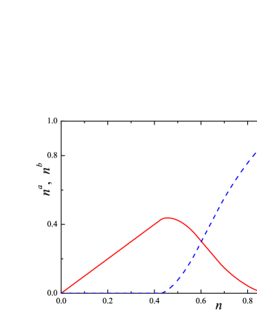
Figure 1: (Color online) Evolution of the occupation numbers of the $a$ and $b$ bands with doping $n$: $n^{a}$ (red) solid line and $n^{b}$ (blue) dashed line. The parameters are $\lambda/w_{a}=0.8$, $\lambda_{b}/w_{a}=2.0$, $K=16w_{a}$ and $w_{b}/w_{a}=0.25$.

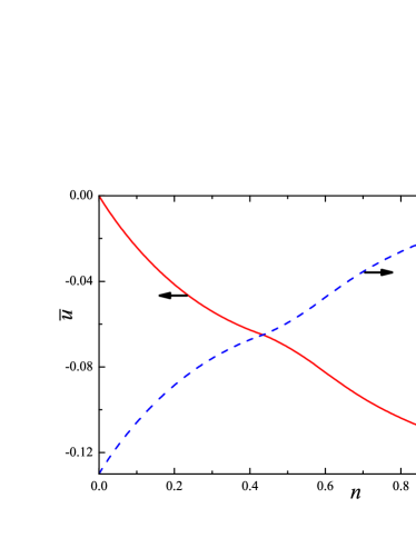
Figure 2: (Color online) The dependence of $\bar{u}$ (solid (red) curve) and $\Delta E_{\rm eff}=-\lambda_{b}\bar{u}$ (dashed (blue) curve) on $n$. The parameters are the same as in Fig 1.

The dependence of $n^{a}$ and $n^{b}$ on doping $n$ is illustrated in Fig. 1. At low doping, the bottom of $b$ band lies far above the bottom of the wider band $a$, and there exist only $a$ electrons. The filling of the bands gives rise to a non-zero strain $\bar{u}$, see Eq. (9), and hence to the band shift $\Delta E_{\rm eff}$. The plots $\bar{u}(n)$ and $\Delta E_{\rm eff}(n)$ are shown in Fig. 2. When $\lambda$ and $\lambda_{b}$ have the same signs the band $b$ shifts downward ($\Delta E_{\rm eff}>0$). Thus, with the increase of $n$, the chemical potential crosses the bottom of the $b$ band and $b$ electrons appear in the system. Due to electron-electron correlations, the effective width of $a$ band starts to decrease. This band narrowing and increase of $\Delta E_{\rm eff}$ leads to decreasing of the number of $a$ electrons, and at some doping level, the charge carriers of type $a$ disappear in the system, see Fig. 1.

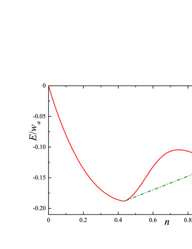
Figure 3: (Color online) The energy of the system vs doping level $n$. Solid (red) curve corresponds to the homogeneous state, whereas the dot-dash (green) curve is the energy of the phase-separated state. The parameters are the same as in Fig 1.

The energy of the system in the homogeneous state,

$$E_{\text{hom}}=\sum_{\alpha}\int\rho_{\alpha}(E^{\prime})E^{\prime}dE^{\prime},$$

is the sum of electron energies in all filled bands. After straightforward calculations, we can write $E_{\text{hom}}$ in the form

$$E_{\text{hom}} = 2g_{a}^{2}w_{a}\left(1-\frac{\lambda\bar{u}}{t_{a}}\right)\varepsilon_{0}\left[\frac{\mu}{g_{a}w_{a}\left(1-\lambda\bar{u}/t_{a}\right)}\right]$$ (19)

$$+ 2g_{b}^{2}w_{b}\varepsilon_{0}\left[\frac{\mu-\lambda_{b}\bar{u}}{g_{b}w_{b}}\right]+\lambda_{b}\bar{u}n_{b}+\frac{K\bar{u}^{2}}{2}\,,$$

where

$$\varepsilon_{0}(\mu^{\prime})=\int\limits_{-1}^{\mu^{\prime}}dE^{\prime}E^{\prime}\,\rho_{0}(E^{\prime})\,.$$ (20)

The dependence of $E_{\text{hom}}(n)$ is shown in Fig. 3 by solid line. We see that within a certain $n$ range the system can have a negative compressibility, $\partial^{2}E_{\text{hom}}/\partial n^{2}<0$, which means a possibility for the charge carriers to form two phases with different electron concentrations tb1 .

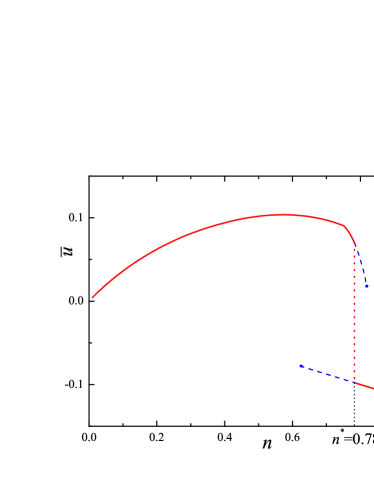
Figure 4: (Color online) Lattice strain as a function of doping. The parameters are $\lambda/w_{a}=-1.2$, $\lambda_{b}/w_{a}=2$, $K=16w_{a}$ and $w_{b}/w_{a}=0.25$. Jump-like transition between two states with different values of lattice distortions occurs at $n=n^{*}$. Solid (red) lines correspond to the states with minimum energy, whereas dashed (blue) lines correspond to metastable states.

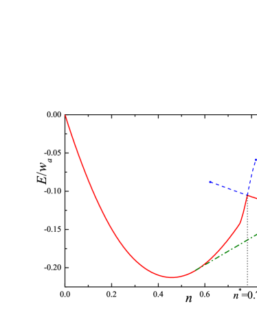
Figure 5: (Color online) The energy of the system vs doping level $n$. Solid (red) curve corresponds to the homogeneous state, whereas the dot-dash (green) curve is the energy of the phase-separated state. The dashed (blue) curves correspond to the energies of metastable states. The parameters are the same as in Fig 4. The kink in the curve $E_{\text{hom}}(n)$ corresponds to the jump-like change in the lattice distortion.

The values of parameters chosen to plot Figs. 1-3 correspond to a continuous evolution of the strain with doping. However, as it was mentioned in Section II, one could also expect a jump-like transition between states with different values of the strains at certain values of parameters. Such a situation is illustrated in Figs. 4 and 5. In Fig. 4, we can see that at some $n=n^{*}$ the strain $\bar{u}$ exhibits a stepwise transition with the change of the sign. In the vicinity of $n^{*}$, there exist two competing states, $A$ and $B$, corresponding to two solutions of the system of equations (9), (15), and (17) for $\bar{u}$, $n^{a}$, $n^{b}$, and $\mu$. In the state $A$, we have $n^{b}\ll n^{a}$ or $n_{b}=0$, whereas in the $B$ state, $b$ electrons are prevailing. The energies of these states coincide at $n=n^{*}$ and at $n>n^{*}$, state $A$ has the a higher energy than state $B$. The minimum energy of the homogeneous state is shown in Fig. 5 by solid line and the energies of the metastable states are depicted by dashed lines. The change in the type of state corresponds to the kink in $E_{\text{hom}}(n)$ curve at $n=n^{*}$.

The existence of two competing states in some range of parameters can be illustrated in the following way. Let us study Hamiltonian (II) where the strain $\bar{u}=u$ is considered as an independent parameter. We analyze this Hamiltonian in the way similar to that described above. Namely, at each given $u$, we solve the system of equations (15) and (17) for $n^{a}$, $n^{b}$, and $\mu$, and then find the system energy per lattice site $E_{hom}(u)$. The optimum value $\bar{u}$ is then determined by minimization of $E_{hom}(u)$. The numerical analysis shows that the function $E_{hom}(u)$ has one or two minima depending on model parameters. The functions $E_{hom}(u)$ calculated for two sets of parameters $\lambda$, $\lambda_{b}$, $K$ and $w_{b}$ at different doping levels $n$ are shown in Figs 6. At $u=\bar{u}$ corresponding to the minimum of $E_{hom}(u)$, we have

$$\frac{\partial E_{hom}}{\partial u}\equiv\frac{1}{N}\left\langle\frac{\partial H_{\text{eff}}}{\partial u}\right\rangle=\lambda z\langle a^{\dagger}_{\mathbf{i}\sigma}a_{\mathbf{j}\sigma}\rangle+\lambda_{b}n^{b}+K\bar{u}=0\,,$$ (21)

and we come back to Eq. (9) for $\bar{u}$.

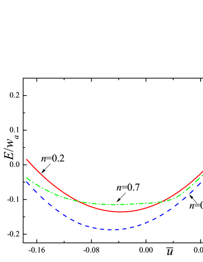
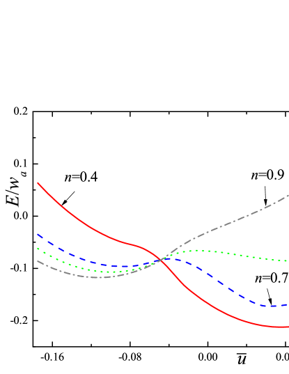
Figure 6: The energies of the homogeneous state depending on the strain $u$ calculated for $\lambda/w_{a}=0.8$ (upper panel), and for $\lambda/w_{a}=-1.2$ (lower panel) at different values of doping $n$. Other parameters are the same for both panels; $\lambda_{b}/w_{a}=2$, $K=16w_{a}$, and $w_{b}/w_{a}=0.25$. In the case of $\lambda/w_{a}=-1.2$, the function $E_{hom}(u)$ has two minima within a certain doping range.

In the general case, it is difficult to find explicit conditions for the existence of the jump-like transition. Here, we analyze the important particular case of $\lambda=0$. Let us consider the function $E^{\prime}(u)\equiv\partial E_{hom}/\partial u$, which now has a form $E^{\prime}(u)=Ku+\lambda_{b}n^{b}(u)$. The $E^{\prime}(u)$ curves calculated at different values of doping are illustrated in Fig. 7. For large negative strain, the $b$ band lies far below the $a$ band, and we have $n^{a}=0$ and $n^{b}=n$. Thus, $E^{\prime}(u)=Ku+\lambda_{b}n$ linearly grows with $u$ up to the point $u=u_{1}$, when the chemical potential $\mu$ reaches the bottom of the effective $a$ band $-g_{a}wa=-(1-n)w_{a}$, and $a$ electrons appear in the system. Using second equation in the system Eq. (15) with $n_{b}=n$, and $\mu=-(1-n)w_{a}$, we obtain the following expression for $u_{1}$:

$$u_{1}=\frac{-1}{\lambda_{b}}\left[(1-n)w_{a}+\left(1-\frac{n}{2}\right)w_{b}\mu_{0}\left(\frac{n}{2-n}\right)\right],$$ (22)

where $-1<\mu_{0}(n)<1$ is the function inverse to $n_{0}(\mu^{\prime})$, Eq. (16). This function is shown in the inset in Fig. 7. For large positive $u$, when band $b$ lies above band $a$, we have $n^{a}=n$ and $n^{b}=0$, and consequently $E^{\prime}(u)=Ku$ linearly decreases with $u$ till the point $u_{2}>u_{1}$, where $b$ electrons appear. Acting in a similar way, we find

$$u_{2}=\frac{1}{\lambda_{b}}\left[(1-n)w_{b}+\left(1-\frac{n}{2}\right)w_{a}\mu_{0}\left(\frac{n}{2-n}\right)\right].$$ (23)

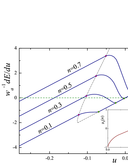
Figure 7: The dependence of $E^{\prime}(u)$ on the strain $u$ at different values of doping $n$. The parameters are $\lambda=0$, $\lambda_{b}/w_{a}=6$, $K=16w_{a}$, and $w_{b}/w_{a}=0.25$. The values of $u_{1}(n)$ and $u_{2}(n)>u_{1}(n)$ are marked by circles. In the inset, the function $\mu_{0}(n)$, inverse to the function (16) is shown.

It is clearly seen from Fig. 7, that if

$$E^{\prime}(u_{1})=Ku_{1}+\lambda_{b}n\geq 0,\;\;E^{\prime}(u_{2})=Ku_{2}\leq 0\,,$$ (24)

then the function $E^{\prime}(u)$ has three zeros, and the energy $E(u)$, in turn, has two minima. Using Eqs. (22) and (23), and taking the equality signs in relations (24), we get the estimate for the minimum value of $\lambda_{b}$, at which the jump-like transition can occur

$$\frac{(\lambda_{b}^{*})^{2}}{K}=\frac{1-n_{2}}{n_{2}}w_{a}\left(1-\frac{w_{b}^{2}}{w_{a}^{2}}\right),$$ (25)

where $n_{2}$ is found from the equation

$$\mu_{0}\left(\frac{n_{2}}{2-n_{2}}\right)=-\frac{1-n_{2}}{1-n_{2}/2}\frac{w_{b}}{w_{a}}.$$ (26)

The value of $\lambda_{b}^{*}$ decreases with $w_{b}$. For very small ratio $w_{b}/w_{a}\ll 1$, we have $\mu_{0}[n_{2}/(2-n_{2})]\approx 0$, that is, $n_{2}\approx 2/3$, and

$$\lambda_{b}^{*}\approx\sqrt{\frac{w_{a}K}{2}}.$$ (27)

Note that the function $E(u)$ can still have two minima when conditions (24) are not met, since the derivative $E^{\prime}(u)$ can continue to grow (decrease) above (below) $u_{1}$ ($u_{2}$), and, consequently, $\lambda_{b}^{*}$ found from these conditions overestimates its value.

For $\lambda=0$ the jump-like transition occurs for relatively large values of $\lambda_{b}$. For example, at $K=16w_{a}$ and $w_{b}=0.25w_{a}$, from Eq. (25) one obtains $\lambda_{b}^{*}\approx 3.6w_{a}$. The numerical analysis shows, however, that even small negative (if $\lambda_{b}>0$) $\lambda$ sufficiently reduces the threshold value of $\lambda_{b}^{*}$. For example, at $\lambda=-0.4w_{a}$, the jump-like behavior arises starting from $\lambda_{b}^{*}\approx 2.0w_{a}$ ($K=16w_{a}$ and $w_{b}=0.25w_{a}$). Thus, different signs of $\lambda$ and $\lambda_{b}$ favor the existence of such transition.

V Conclusions

The electron-lattice interaction plays an important role in the systems with strongly correlated electrons affecting their behavior with doping. The interaction of electrons with the lattice distortions results, first, in the hopping probability and, second, in the relative shifts of the electronic bands. We analyzed the problem in the framework of the two-band Hubbard model. We demonstrated that if the electron-lattice interaction is strong enough, there appears a competition between states with different values of strains and the transition between these states can occur in a jump-like manner. We also showed that the electron-lattice interaction produces a pronounced effect on the conditions of the electronic phase separation since it influences the value of the bandwidth ratio and the relative positions of the bands.

References

- (1) E. Dagotto, Nanoscale Phase Separation and Colossal Magnetoresistance: The Physics of Manganites and Related Compounds (Springer-Verlag, Berlin, 2003).
- (2) E. Dagotto, Science 309, 257 (2005).
- (3) D.I. Khomskii, Phys. Scripta 72, CC8 (2005).
- (4) T. Egami and Despina Louca, J. Supercond. 12, 23 (1999).
- (5) T. Egami, J. Supercond. Nov. Magn. 19, 203 (2006).
- (6) P.W. Anderson, Science 235, 1196 (1987).
- (7) C.M. Varma, S. Schmitt-Rink, and E. Abrahams, Solid State Comm. 62, 681 (1987).
- (8) J. Wagner, W. Hanke, and D.J. Scalapino, Phys. Rev. B43, 10517 (1991).
- (9) A.O. Sboychakov, K.I. Kugel, and A.L. Rakhmanov Phys. Rev. B76, 195113 (2007).
- (10) K.I. Kugel, A.L. Rakhmanov, and A.O. Sboychakov, Phys. Rev. Lett. 95,267210 (2005); A.O. Sboychakov, K.I. Kugel, and A.L. Rakhmanov, Phys. Rev. B74, 014401 (2006).
- (11) K.I. Kugel, A.L. Rakhmanov, A.O. Sboychakov, and D.I. Khomskii, Phys. Rev. B78, 155113 (2008); K.I. Kugel, A.O. Sboychakov, and D.I. Khomskii, J. Supercond. Nov. Magn. 22, 147 (2009).
- (12) A.O. Sboychakov, K.I. Kugel, A.L. Rakhmanov, and D.I. Khomskii, Phys. Rev. B80, 024423 (2009).
- (13) R. Suzuki, T. Watanabe, and S. Ishihara, Phys. Rev. B80, 054410 (2009).
- (14) K. Yonemitsu, A.R. Bishop, and J. Lorenzana, Phys. Rev. Lett. 69, 965 (1992); Phys. Rev. B47, 12059 (1993).
- (15) P. Piekarz, J. Konior, and J.H. Jefferson, Phys. Rev. B59, 14697 (1999).
- (16) A.O. Sboychakov, Sergey Savel’ev, A.L. Rakhmanov, K.I. Kugel, and Franco Nori, Phys. Rev. B77, 224504 (2008).
- (17) T.V. Ramakrishnan, H.R. Krishnamurthy, S.R. Hassan, G.V. Pai, Phys. Rev. Lett. 92, 157203 (2004).
- (18) K.I. Kugel, A.L. Rakhmanov, A.O. Sboychakov, Nicola Poccia, Antonio Bianconi, Phys. Rev. B78, 165124 (2008).
- (19) J. Hubbard, Proc. Roy. Soc. (London) A276, 238 (1963).