Abstract

Recently a new approach to inflation proposal has been constructed via the smeared coherent state picture of spacetime noncommutativity. Here we generalize this viewpoint to a Randall-Sundrum II braneworld scenario. This model realizes an inflationary, bouncing solution without recourse to any axillary scalar or vector fields. There is no initial singularity and the model has the potential to produce scale invariant spectrum of scalar perturbations.
PACS: 02.40.Gh,  11.10.Nx,  04.50.-h,  98.80.Cq
Key Words: Noncommutative Geometry, Inflation, Braneworld Cosmology

1 Introduction

Spacetime non-commutativity can be achieved naturally on certain backgrounds of string theory [1,2]. Existence of a fundamental minimal length of the order of the Planck length and spacetime non-commutativity are naturally related in these theories [3]. In this viewpoint, description of the spacetime as a smooth commutative manifold becomes therefore a mathematical assumption no more justified by physics. It is then natural to relax this assumption and conceive a more general noncommutative spacetime, where uncertainty relations and spacetime discretization naturally arise. Noncommutativity is the central mathematical concept expressing uncertainty in quantum mechanics, where it applies to any pair of conjugate variables, such as position and momentum. One can just as easily imagine that position measurements might fail to commute and describe this using noncommutativity of the coordinates. The noncommutativity of spacetime can be encoded in the commutator [1]

$$[\hat{x}^{i},\hat{x}^{j}]=i\theta^{ij}$$ (1)

where $\theta^{ij}$ is a real, antisymmetric and constant tensor, which determines the fundamental cell discretization of spacetime much in the same way as the Planck constant $\hbar$ discretizes the phase space. In $d=4$, it is possible by a choice of coordinates to bring some $\theta^{ij}$s to the following form

$$\theta^{ij}=\left(\begin{array}[]{cccc}0&\theta&0&0\\ -\theta&0&\theta&0\\ 0&-\theta&0&\theta\\ 0&0&-\theta&0\end{array}\right)$$

This was motivated by the need to control the divergences showing up in theories such as quantum electrodynamics. Here $\sqrt{\theta}$ is the fundamental minimal length ( order of magnitude of $\sqrt{\theta}$ can be found in Ref. [3]). This noncommutativity leads to the modification of Heisenberg uncertainty relation in such a way that prevents one from measuring positions to better accuracies than the Planck length.

It has been shown that noncommutativity eliminates point-like structures in the favor of smeared objects in flat spacetime. As Nicolini et al.  have shown [4] ( see also [5] for extensions ), the effect of smearing is mathematically implemented as a substitution rule: position Dirac-delta function is replaced everywhere with a Gaussian distribution of minimal width $\sqrt{\theta}$. In this framework, they have chosen the mass density of a static, spherically symmetric, smeared, particle-like gravitational source as follows

$$\rho_{\theta}(r)=\frac{M}{(2\pi\theta)^{\frac{3}{2}}}\exp(-\frac{r^{2}}{4\theta}).$$ (2)

As they have indicated, the particle mass $M$, instead of being perfectly localized at a point, is diffused throughout a region of linear size $\sqrt{\theta}$. This is due to the intrinsic uncertainty as has been shown in the coordinate commutators (1).

Recently, a new approach to the issue of inflation in the framework of Nicolini et al.  coherent states viewpoint of noncommutativity has been reported by Rinaldi [6]. In this model, the intrinsic noncommutative structure of spacetime is responsible for a violation of the dominant energy condition near the initial singularity, which induces a bounce. The following expansion is quasi-exponential and it does not require any ad hoc scalar field. Here we are going to investigate the effects of the spacetime non-commutativity on the inflationary dynamics in the Randall-Sundrum II braneworld scenario. We use the Nicolini et al. coherent state approach encoded in the smeared picture defined in (2). Some other studies of the non-commutative inflation with different approaches can be found in Ref. [7].

2 Noncommutative brane inflation

We begin with the Randall-Sundrum II (RS II) geometry. In this setup, there is a single positive tension brane embedded in an infinite bulk [8]. The Friedmann equation governing the evolution of the brane in this scenario is given as follows ( see for instance [9])

$$H^{2}=\frac{\Lambda_{4}}{3}+\bigg{(}\frac{8\pi}{3M^{2}_{4}}\bigg{)}\rho+\bigg{(}\frac{4\pi}{3M^{3}_{5}}\bigg{)}\rho^{2}+\frac{{\cal{E}}_{0}}{a^{4}}$$ (3)

Where $M_{4}$ and $M_{5}$ are four and five dimensional fundamental scales respectively and $\Lambda_{4}$ is the effective cosmological constant on the brane. The last term in equation (3) is called the dark radiation term and ${\cal{E}}_{0}$ is an integration constant. The relation between four and five dimensional fundamental scales is

$$M_{4}=\sqrt{\frac{3}{4\pi}}\bigg{(}\frac{M^{2}_{5}}{\sqrt{\lambda}}\bigg{)}M_{5}$$ (4)

where $\lambda$ is the brane tension. We now suppose that the initial singularity that leads to RS II geometry afterwards, is smeared due to noncommutativity of the spacetime. A newly proposed model for the similar scenario in the usual 4D universe suggests that one could split the energy density on any hypersurface as [6]

$$\rho=\rho_{0}e^{-|\tau|^{2}/4\theta}e^{-|\vec{{X}}|^{2}/4\theta}$$ (5)

where $R^{2}=\tau^{2}+|\vec{X}|^{2}$ and $\tau=it$ is the Euclidean time. Note that we suppose that the universe enters the RS II geometry immediately after the initial smeared singularity which is a reasonable assumption ( for instance, from a M-theory perspective of the cyclic universe this assumption seems to be reliable, see Ref. [10]). From one hypersurface to another, the $\vec{X}$-dependent part of $\rho$ does not change, so it can be included into $\rho_{0}$. If we neglect the dark radiation term (which is reasonable during inflation as it is vanishing really fast) and also the brane cosmological constant, the Friedmann equation (3) can be rewritten as

$$H^{2}=\frac{8\pi}{3M^{2}_{4}}\rho\bigg{[}1+\frac{\rho}{2\lambda}\bigg{]}$$ (6)

Using equation (5), this Friedmann equation in noncommutative space could be rewritten as follows

$$\bigg{(}\frac{\dot{a}}{a}\bigg{)}^{2}=\frac{8\pi}{3M^{2}_{4}}\rho_{0}e^{-t^{2}/4\theta}\bigg{[}1+\frac{\rho_{0}e^{-t^{2}/4\theta}}{2\lambda}\bigg{]}.$$ (7)

This equation can be solved for $a(t)$ to obtain

$$a\left(t\right)={\cal{H}}\bigg{(}\Big{[}\frac{1}{4}\,{\frac{\rho_{0}-2\,\sqrt{2}\theta\,{\lambda}^{3/2}\sqrt{\frac{8\pi}{3M^{2}_{4}}}}{\rho_{0}}}\Big{]}\,,\,\,\Big{[}\frac{1}{2}\Big{]}\,,\,\,\frac{1}{8}\,{\frac{\sqrt{2}\sqrt{\frac{8\pi}{3M^{2}_{4}}}\left[\left(4\,\rho_{0}+4\,\lambda\right)\theta+t\rho_{0}\right]^{2}}{\theta\,\sqrt{\lambda}\rho_{0}}}\bigg{)}\times$$

$${\exp\bigg{\{}-\frac{1}{16}\,{\frac{\left[\left(8\,\rho_{0}+8\,\lambda\right)\theta+t\rho_{0}\right]\sqrt{2}\sqrt{\frac{8\pi}{3M^{2}_{4}}}t}{\theta\,\sqrt{\lambda}}}}\bigg{\}}\,\,\,+$$

$$\left[\left(4\,\rho_{0}+4\,\lambda\right)\theta+t\rho_{0}\right]{\exp\bigg{\{}-\frac{1}{16}\,{\frac{\left[\left(8\,\rho_{0}+8\,\lambda\right)\theta+t\rho_{0}\right]\sqrt{2}\sqrt{\frac{8\pi}{3M^{2}_{4}}}t}{\theta\,\sqrt{\lambda}}}}\bigg{\}}\times$$

$${\cal{H}}\bigg{(}\Big{[}\frac{1}{4}\,{\frac{3\,\rho_{0}-2\,\sqrt{2}\theta\,{\lambda}^{3/2}\sqrt{\frac{8\pi}{3M^{2}_{4}}}}{\rho_{0}}}\Big{]}\,,\,\,\Big{[}\frac{3}{2}\Big{]}\,,\,\,\frac{1}{8}\,{\frac{\sqrt{2}\sqrt{\frac{8\pi}{3M^{2}_{4}}}\left[\left(4\,\rho_{0}+4\,\lambda\right)\theta+t\rho_{0}\right]^{2}}{\theta\,\sqrt{\lambda}\rho_{0}}}\bigg{)}\,,$$ (8)

where ${\cal{H}}$ shows the Hypergeometric function of the arguments. To see the cosmological dynamics of the model, we plot the evolution of the scale factor and the Hubble parameter in figures $1$ and $2$. As figure $1$ shows, this noncommutative model naturally gives an inflation era without consulting to any axillary inflaton field. On the other hand, due to smeared picture adopted in this noncommutative framework, there is no initial singularity in this setup.

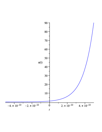
Figure 1: Evolution of the scale factor in noncommutative Randall-Sundrum II geometry. There is an inflationary era without recourse to any scalar or vector fields. The model avoids also the initial singularity.

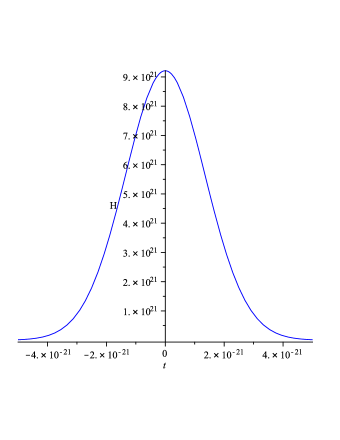
Figure 2: Evolution of the Hubble parameter in noncommutative Randall-Sundrum II geometry

The number of e-folds in this model will be given by

$$N=\int^{t_{f}}_{t_{i}}Hdt\simeq\frac{8}{3}\pi\,{\it\rho_{0}}\,\bigg{[}\sqrt{\pi\theta}\,\,\,{\rm erf}\Big{(}\frac{1}{2}\,{\frac{t_{f}}{\sqrt{\theta}}}\Big{)}+\frac{1}{2}\,\sqrt{2\pi\theta}\,\,\,{\rm erf}\Big{(}\frac{1}{2}\,{\frac{\sqrt{2}t_{f}}{\sqrt{\theta}}}\Big{)}{\lambda}^{-1}\bigg{]}{M_{4}}^{-2}$$

$$-\frac{8}{3}\,\pi\,{\it\rho_{0}}\,\bigg{[}\sqrt{\pi\theta}\,\,\,{\rm erf}\Big{(}\frac{1}{2}\,{\frac{t_{i}}{\sqrt{\theta}}}\Big{)}+\frac{1}{2}\,\sqrt{2\pi\theta}\,\,\,{\rm erf}\Big{(}\frac{1}{2}\,{\frac{\sqrt{2}t_{i}}{\sqrt{\theta}}}\Big{)}{\lambda}^{-1}\bigg{]}{M_{4}}^{-2}.$$ (9)

By expanding the error functions in equation (9) in series, the number of e-folds (supposing that the universe enters the inflationary phase immediately after the big bang,  that is,  $t_{i}=0$ and $t_{f}=t$) will be given by

$$N\simeq\frac{8}{3}\,\pi\,{\it\rho_{0}}\,\bigg{[}t-\frac{1}{12}\,{\frac{{t}^{3}}{\sqrt{\pi}{\theta}^{\frac{3}{2}}}}+{\frac{1}{160}}\,{\frac{{t}^{5}}{\sqrt{\pi}{\theta}^{\frac{5}{2}}}}+\frac{1}{2}\,\Big{(}2\,t-\frac{1}{6}\,{\frac{\sqrt{2}{t}^{3}}{\sqrt{\pi}{\theta}^{\frac{3}{2}}}}+\frac{1}{40}\,{\frac{\sqrt{2}{t}^{5}}{\sqrt{\pi}{\theta}^{\frac{5}{2}}}}\Big{)}{\lambda}^{-1}\bigg{]}{M_{4}}^{-2}.$$ (10)

We plot this relation as a function of time in figure (3). It is obvious from this figure that if $\rho_{0}$ is suitably large, we will get sufficient amount of inflation in this scenario.

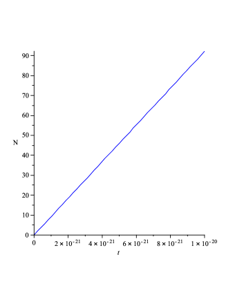
Figure 3: Number of e-folds as a function of time. If the amount of $\frac{\rho_{0}}{\lambda}$ in equation (10) is suitably large, we will get sufficient amount of inflation. We have set $\theta=10^{-20}$ and $\frac{\rho_{0}}{\lambda}=10^{16}$ with $M_{4}=1$.

Now, using equation (10) and solving for $\rho_{0}$, we find

$$\rho_{0}=45\,\sqrt{\theta}\lambda\,{M_{4}}^{2}\bigg{[}2\,{\pi}^{\frac{3}{2}}\theta\,\lambda\,t\,\,\,{\rm erf}\Big{(}\frac{1}{2}\,{\frac{t}{\sqrt{\theta}}}\Big{)}+4\,\pi\,{\theta}^{\frac{3}{2}}\lambda\,{e^{-\frac{1}{4}\,{\frac{{t}^{2}}{\theta}}}}+{\pi}^{\frac{3}{2}}\theta\,\sqrt{2}t\,\,\,{\rm erf}\Big{(}\frac{1}{2}\,{\frac{\sqrt{2}t}{\sqrt{\theta}}}\Big{)}+2\,\pi\,{\theta}^{\frac{3}{2}}{e^{-\frac{1}{2}\,{\frac{{t}^{2}}{\theta}}}}\bigg{]}^{-1}.$$ (11)

Usually the number of e-folds required to solve problems of standard cosmology is $N\simeq 60-70$. If we assume that the value of  $\theta$  to be of the order of $10^{-20}$, the value of $\frac{\rho_{0}}{\lambda}$ required for a successful inflation with $N=60$ is $\frac{\rho_{0}}{\lambda}\sim 10^{16}$ where we have set $M_{4}=1$. We note that $\frac{\rho_{0}}{\lambda}$ obtained in this way is a fine-tuned value. The value of  $\theta$  can be estimated for instance by the noncommutative correction to the planets perihelion precession of the solar system [12] (see also [3]). Another point we stress here is that Rinaldi has pointed in Ref. [6] that $\frac{\rho_{0}}{\lambda}$ may play the role of a cosmological constant after the inflationary phase. Actually this is not the case since $\frac{\rho_{0}}{\lambda}$ has not correct equation of state to be dark energy.

To be a realistic model of the early universe and also to test whether or not our model is consistent with recent observational data, a scale invariant spectrum of scalar perturbations should be generated after inflation. We define the slow-roll parameters as usual

$$\epsilon\equiv\frac{{M_{4}}^{2}}{4\pi}\bigg{(}\frac{H^{\prime}}{H}\bigg{)}^{2},$$

$$\eta\equiv\frac{{M_{4}}^{2}}{4\pi}\bigg{(}\frac{H^{\prime\prime}}{H}\bigg{)}$$ (12)

These slow-roll parameters as a function of cosmic time are given in appendix $1$. We assume that as usual the scalar spectral index is given by the

$$n_{s}-1\simeq-6\epsilon+2\eta.$$ (13)

This assumption will be justified shortly. To match the observational data, $n_{s}$ should be around unity at the end of inflation. This guaranties the generation of scale invariant scalar perturbations. Figure $4$ shows variation of $n_{s}$ versus the cosmic time. In plotting this figure we have used the same values of parameters as have been used to plot figure $3$. As one can see from this figure, it is possible essentially to have scale invariant scalar spectrum in this model. However, we stress that in order to study the power spectrum in our model, a more thorough analysis of generation of density perturbations should be done, taking into account the dark radiation term since this term plays a crucial role in perturbations. Especially the relation (13) needs to be reformulated in this non-commutative framework. These issues are under investigation by the authors.

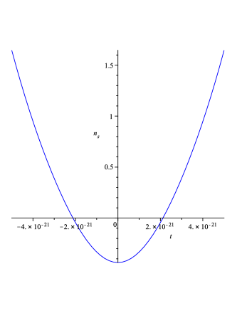
Figure 4: Variation of the scalar spectral index versus the cosmic time. The spectral index approaches the Harrison-Zel’dovic spectrum at the end of inflation. The parameters used to plot this figure are the same as previous figures. The spectral index is exactly one at $t=\pm 4.021168857\times 10^{-21}$

Finally, two points should be explained here: Firstly, one might think that this model has the potential to be able to solve the flatness problem from an accelerated expansion. We note however that this is not actually the case since as long as this model want to address the singularity problem, one needs to consider $t\rightarrow-\infty$, where $\rho$ (defined in Eq. (5)) is exponentially small. If there were large spatial curvature when $t\rightarrow-\infty$, the spatial curvature will dominate the universe quickly. Secondly, as one can read from Fig. $2$, with our choice of parameters, the end of the inflation era takes place around $4\times 10^{-21}$. In order to have a scale invariant spectrum of scalar perturbations, $n_{s}$ should be around unity at this time. From figure $4$ one can see that this is indeed the case. The scalar spectral index is exactly one at the time $t=\pm 4.021168857\times 10^{-21}$. $n_{s}$ changes from negative values at $t=0$ to around unity at the end of inflationary era.

3 Summary

In this letter, by adopting the smeared coherent state picture of spacetime noncommutativity, we generalized the Randall-Sundrum II braneworld inflation to noncommutative spaces. This model realizes an inflationary, bouncing solution without recourse to any axillary scalar or vector fields. Due to noncommutative structure of the very spacetime which admits the existence of a fundamental length scale, there is no initial singularity in this model. Note that we supposed that the universe enters the RS II geometry immediately after the initial smeared singularity which is a reasonable assumption for instance from a M-theory perspective of the cyclic universe. There is a parameter, $\frac{\rho_{0}}{\lambda}$, in this model that has the potential to play important roles in the inflation era: by taking the number of e-folds to be $N\simeq 60$, and setting the noncommutativity parameter to be $\theta\sim 10^{-20}$, the value of $\frac{\rho_{0}}{\lambda}$ required for a successful inflation is $\frac{\rho_{0}}{\lambda}\sim 10^{16}$. By treating the scalar perturbations in this setup, we have shown that it is possible essentially to have scale invariant scalar perturbations in this framework. From another viewpoint, $\rho_{0}$ contains a space-dependent part of $e^{-|\vec{{X}}|^{2}/4\theta}$ that essentially breaks the homogeneity on the successive hypersurfaces. This may open new windows on the issue of cosmological perturbations. A more thorough analysis of perturbations on the brane is therefore required to justify the successes of this model.

Appendix 1
Slow-roll Parameters

The slow-roll parameters defined in equation (12) are given by

$$\epsilon=\frac{{M_{4}}^{2}}{4\pi}{\frac{9}{64}}\,\Bigg{[}-\frac{4}{3}\,\pi\,{\rho_{0}}\,t{{\rm e}^{-\frac{1}{4}\,{\frac{{t}^{2}}{\theta}}}}\left(1+{{\rm e}^{-\frac{1}{4}\,{\frac{{t}^{2}}{\theta}}}}{\lambda}^{-1}\right){\theta}^{-1}{M_{4}}^{-2}-\frac{4}{3}\,\pi\,{\rho_{0}}\,{{\rm e}^{-\frac{1}{2}\,{\frac{{t}^{2}}{\theta}}}}t{\theta}^{-1}{\lambda}^{-1}{M_{4}}^{-2}\Bigg{]}^{2}\times$$

$$\Bigg{[}{M_{4}}^{4}{\pi}^{-2}{\rho_{0}}^{-2}{{\rm e}^{-\frac{1}{2}\,{\frac{{t}^{2}}{\theta}}}}\left(1+{{\rm e}^{-\frac{1}{4}\,{\frac{{t}^{2}}{\theta}}}}{\lambda}^{-1}\right)^{-2}\Bigg{]}\,$$ (14)

and

$$\eta=\frac{{M_{4}}^{2}}{4\pi}\frac{3}{8}\,\Bigg{[}-\frac{4}{3}\,\pi\,{\rho_{0}}\,{{\rm e}^{-\frac{1}{4}\,{\frac{{t}^{2}}{\theta}}}}\left(1+{{\rm e}^{-\frac{1}{4}\,{\frac{{t}^{2}}{\theta}}}}{\lambda}^{-1}\right){\theta}^{-1}{M_{4}}^{-2}+\frac{2}{3}\,\pi\,{\rho_{0}}\,{t}^{2}{{\rm e}^{-\frac{1}{4}\,{\frac{{t}^{2}}{\theta}}}}\left(1+{{\rm e}^{-\frac{1}{4}\,{\frac{{t}^{2}}{\theta}}}}{\lambda}^{-1}\right){\theta}^{-2}{M}^{-2}$$

$$+2\,\pi\,{\rho_{0}}\,{t}^{2}{{\rm e}^{-\frac{1}{2}\,{\frac{{t}^{2}}{\theta}}}}{\theta}^{-2}{\lambda}^{-1}{M_{4}}^{-2}-\frac{4}{3}\,\pi\,{\rho_{0}}\,{{\rm e}^{-\frac{1}{2}\,{\frac{{t}^{2}}{\theta}}}}{\theta}^{-1}{\lambda}^{-1}{M}^{-2}\Bigg{]}\times$$

$$\Bigg{[}{M_{4}}^{2}{\pi}^{-1}{\rho_{0}}^{-1}{{\rm e}^{\frac{1}{4}\,{\frac{{t}^{2}}{\theta}}}}\left(1+{{\rm e}^{-\frac{1}{4}\,{\frac{{t}^{2}}{\theta}}}}{\lambda}^{-1}\right)^{-1}\Bigg{]}\,.$$ (15)

References

-
[1]
M. R. Douglas and N. A. Nekrasov, Rev. Mod. Phys. 73
(2001) 977-1029
R. J. Szabo, Phys. Rept. 378 (2003) 207-299
N. Seiberg and E. Witten, JHEP 9909 (1999) 032
A. Connes and M. Marcolli, arXiv:math.QA/0601054
A. Connes, J. Math. Phys. 41 (2000) 3832-3866
A. Konechny and A. Schwarz, Phys. Rept. 360 (2002) 353-465
M. Chaichian et al, Eur. Phys. J. C 29 (2003) 413-432
F. Ardalan, H. Arfaei and M. M. Sheikh-Jabbari, JHEP 9902 (1999) 016
A. Micu and M. M. Sheikh-Jabbari, JHEP 0101 (2001) 025 -
[2]
G. Veneziano, Europhys. Lett. 2 (1986) 199
D. Amati, M. Ciafaloni and G. Veneziano, Phys. Lett. B 197 (1987) 81
D. Amati, M. Ciafaloni and G. Veneziano, Int. J. Mod. Phys. A 3 (1988) 1615
D. Amati, M. Ciafaloni and G. Veneziano, Nucl. Phys. B 347 (1990) 530
D. J. Gross and P. F. Mende, Nucl. Phys. B 303 (1988) 407
D. Amati, M. Ciafaloni and G. Veneziano, Phys. Lett. B 216 (1989) 41 -
[3]
K. Nozari, Far East J. Dynaamical System 9, No.3 (2007)
379-389
P. Nicolini, Int. J. Mod. Phys. A 24 (2009) 1229-1308, [arXiv:0807.1939] -
[4]
P. Nicolini et al., Phys. Lett. B 632 (2006)
547-551
P. Nicollini, J. Phys. A 38 (2005) L631-L638
E. Spallucci, A. Smailagic and P. Nicolini, Phys. Rev. D 73 (2006) 084004 -
[5]
T. G. Rizzo, JHEP 09 (2006) 021
S. Ansoldi, P. Nicolini, A. Smailagic and E. Spallucci, Phys. Lett. B 645 (2007) 261-266
E. Spallucci, A. Smailagic, P. Nicolini, Phys. Lett. B 670 (2009) 449-454
K. Nozari and S.H. Mehdipour, Class. Quantum Grav. 25 (2008) 175015
K. Nozari and S. H. Mehdipour, JHEP 0903 (2009) 061 - [6] M. Rinaldi, [arXiv:0908.1949].
-
[7]
J. Martin and R. Brandenberger, Phys. Rev. D 68 (2003)
0305161
R. Brandenberger, arXiv:[hep-th/0210186v2]
S. Tsujikawa, R. Maartens, R. Brandenberger, Phys. Lett. B 574 (2003) 141
Q. G. Huang and M. Li, JCAP 11 (2003) 001
X. Zhang, JCAP 12 (2006) 002
W. Xue, B. Chen and Y. Wang, JCAP 09 (2007) 011
S. Koh and R. Brandenberger,JCAP 0706 (2007) 021
S. Koh and R. Brandenberger,JCAP 0711 (2007) 013
- [8] L. Randall and R. Sundrum, Phys. Rev. Lett. 83 (1999) 4690, [arXiv:hep-th/9906064].
- [9] R. Maartens, D. Wands, B. A. Bassett and I. Heaard, Phys. Rev. D 62 (2000) 041301
-
[10]
P. J. Steinhardt and N. Turok, Phys. Rev. D 65 (2002)
126003
P. J. Steinhardt and N. Turok, Nucl. Phys. Proc. Suppl. 124 (2003) 38
J. Khoury, P. J. Steinhardt and N. Turok, Phys. Rev. Lett. 92 (2004) 031302
N. Turok and P. J. Steinhardt, Phys. Scripta T117 (2005) 76
M. Bojowald, R. Maartens and P. Singh, Phys. Rev. D 70 (2004) 083517. - [11] B. Gumjudpai, R. Maartens and C. Gordon, Class. Quant. Grav. 20 (2003) 3295, [arXiv:gr-qc/0304067]. See also R. Maartens, [arXiv:astro-ph/0402485].
- [12] K. Nozari and S. Akhshabi, Europhys. Lett. 80 (2007) 20002, [arXiv:0708.3714].