Time-dependent transport in graphene nanoribbons

Abstract

We theoretically investigate the time-dependent ballistic transport in metallic graphene nanoribbons after the sudden switch-on of a bias voltage $V$. The ribbon is divided in three different regions, namely two semi-infinite graphenic leads and a central part of length $L$, across which the bias drops linearly and where the current is calculated. We show that during the early transient time the system behaves like a graphene bulk under the influence of a uniform electric field $E=V/L$. In the undoped system the current does not grow linearly in time but remarkably reaches a temporary plateau with dc conductivity $\sigma_{1}=\pi e^{2}/2h$, which coincides with the minimal conductivity of two-dimensional graphene. After a time of order $L/v_{F}$ ($v_{F}$ being the Fermi velocity) the current departs from the first plateau and saturates at its final steady state value with conductivity $\sigma_{2}=2e^{2}/h$ typical of metallic nanoribbons of finite width.

The recent isolation of single layers of carbon atomsgraph1 has attracted growing attention in the transport properties of graphene-based devices. In these systems unconventional phenomena like the half-integer quantum Hall effectqhe and the Klein tunnelingklein have been observed. Such peculiar behavior stems from the relativistic character of the electrons in the carbon honeycomb lattice. Closed to Dirac point the charge carriers behave as two-dimensional (2D) massless Dirac fermionsreview and have very high mobilitymorozov . This fact has stimulated theoretical and experimental investigations into graphenic ultrafast devicesthz0 like field effect transistorsfet , p-n junction diodes and THz detectorsthz1 ; thz2 . In these systems it is crucial to have full control of the electronic response after the sudden switch-on of an external perturbation, and the study of the real-time dynamics is becoming increasingly important. The investigation of the transient response also is of fundamental interest. One of the most debated aspects of the transport properties of graphene is the minimum conductivity $\sigma_{\mathrm{min}}$ at the Dirac point. From the theoretical point of view the problem arises from the fact that the value of $\sigma_{\mathrm{min}}$ is sensitive to the order in which certain limits (zero disorder and zero frequency) are takenziegler , thus producing different values around the quantum $e^{2}/h$ziegler ; peres ; varlamov ; beenakker . Very recently Lewkowicz and Rosenten overcame this ambiguity employing a time-dependent approach in which the dc conductivity is calculated by solving the quench dynamics of 2D Dirac excitations after the sudden switching of a constant electric field. Interestingly their approach does not suffer from the use of any regularization related to the Kubo or Landauer formalism and yields $\sigma_{\mathrm{min}}=\pi e^{2}/2h$. Despite the large effort devoted to the study of the transport properties of graphenic systems, a genuine real-time analysis which treats on equal footing transients effects and the long-time response of graphene nanoribbons in contact with semi-infinite reservoirs is still missing.

In this Letter we study the time-dependent transport properties of undoped graphene nanoribbons with finite width and virtually infinite length after the sudden switch-on of an external bias voltage. The geometry that we consider is sketched in Fig.1. The nanoribbon is divided in three regions, namely a left (L) and a right (R) semi-infinite graphenic reservoirs and a central (C) region of length $L=aN_{c}$, where $N_{c}$ is the number of cells along the longitudinal $x$ direction and $a=2.46$ Å  is the graphene lattice constant. The width of the ribbon is $W=a\sqrt{3}N_{y}$, where $N_{y}$ is the number of cells along the transverse $y$ direction, in which periodic boundary conditions are imposedblanter ; katnelson ; guinea . The three regions are linked via transparent interfaces, in such a way that in equilibrium the system is translationally invariant along the $x$ direction, see Fig.1.

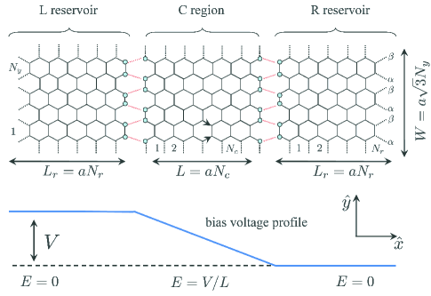
Figure 1: Schematic representation of the system. The nanoribbon has semi-infinite L a nd R graphenic reservoirs and periodic boundary conditions are imposed along the $y$ direction. The bias voltage profile with a linear drop inside the C region is also shown.

Once the system is driven out of equilibrium, the quench dynamics involves high energy excitations and the Dirac-cone approximation, which is valid only at energies lower than 1 eV, is inaccurate. For this reason we adopt a tight-binding description of the system, with Hamiltonian given by

$$H=H_{0}+U(t)=v\sum_{\langle i,j\rangle}c^{\dagger}_{i}c_{j}+\theta(t)\sum_{i}V_{i}c^{\dagger}_{i}c_{i}\,,$$ (1)

where the spin index has been omitted and $v=2.7$ eV is the hopping integral of graphene. The first sum runs over all the pairs of nearest neighbor sites of the ribbon honeycomb lattice and $c^{(\dagger)}_{i}$ is the annihilation (creation) operator of a $\pi$ electron on site $i$. Here we use the collective index $i=\{p,i_{y},i_{x}\}$ to identify a site in the nanoribbon such that $p=\alpha,\beta$ indicates the two inequivalent longitudinal zig-zag chains, $i_{y}$ denotes the cell in the $y$ direction, and $i_{x}$ is the position in the $x$ direction. $H_{0}$ describes the translationally invariant equilibrium system, while $U(t)$ is the bias perturbation with (non self-consistent) voltage profilelineardrop ; lineardrop1 ; lineardrop2 given by the function $V_{i}$

$$V_{i}=\left\{\begin{array}[]{ll}V/2&\quad i\in\mathrm{L}\\ V/2-E\,i_{x}&\quad i\in\mathrm{C}\\ -V/2&\quad i\in\mathrm{R}\end{array}\right.\,,$$ (2)

where $V$ is the total applied voltage and $i_{x}\in(0,L)$ is the $x$-coordinate of the site $i$ in the C region, which is subject to the uniform electric field $E=V/L$ (see Fig.1). The above modelling of the bias profile could find an approximate realization, e.g., in a planar junction in which the L and R regions of the nanoribbon are on top of metallic electrodes.

The time-dependent total current $I(t)$ flowing across the interface in the middle of the C region is written as

$$I(t)=2\sum_{i_{y}=1}^{N_{y}}\sum_{p=\alpha,\beta}I^{(p)}_{i_{y}}(t)\,,$$ (3)

where the factor 2 accounts for the spin degeneracy and $I^{(p)}_{i_{y}}$ is the current flowing across the $p=\alpha,\beta$ chain in the $i_{y}$-th cell, in the middle of the C region (see Fig.1).

Since periodic boundary conditions are imposed along the $y$ direction, the current $I^{(p)}_{i_{y}}$ does not depend on the cell and chain indices $i_{y}$ and $p$, and hence $I(t)=4N_{y}\bar{I}(t)$, where we have defined $\bar{I}\equiv I^{(\alpha)}_{i_{y}}=I^{(\beta)}_{i_{y}}$ for any $i_{y}$.

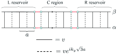
Figure 2: Ladder model for fixed transverse momentum $k_{y}$. The bias profile is the same as in Fig.1.

Since the transverse momentum $k_{y}=2\pi n/\sqrt{3}aN_{y}$ (with $n=0,\dots N_{y}-1$) is conserved the current $\bar{I}$ can be written as

$$\bar{I}(t)=\frac{1}{N_{y}}\sum_{k_{y}}\bar{I}_{k_{y}}(t)\,.$$ (4)

It is seen that the total current of the original $N_{y}$-wide problem can be calculated by summing the currents $\bar{I}_{k_{y}}$ coming from $N_{y}$ independent 1-wide ladder problemsblanter with staggered $k_{y}$-dependent transverse hopping (see Fig.2), with the same bias profile as in Eq.(2).

In order to calculate $\bar{I}_{k_{y}}$ it is convenient to introduce the $y$-Fourier transform of the original electron operators $c_{\{p,k_{y},i_{x}\}}=(N_{y})^{-1/2}\sum_{i_{y}}e^{ik_{y}i_{y}\sqrt{3}a}c_{\{p,i_{y},i_{x}\}}$ in terms of which the current $\bar{I}_{k_{y}}$ can be cast as

$$\bar{I}_{k_{y}}(t)=\frac{2\,e\,v}{\hbar}\mathrm{Re}\left[G^{<}_{\{p,k_{y},\frac{L}{2}\};\{p,k_{y},\frac{L}{2}+\frac{a}{2}\}}(t,t)\right]\,,$$ (5)

where $G^{<}$ is the lesser Keldysh Green’s function

$$G^{<}_{\{p,k_{y},i_{x}\};\{r,q_{y},j_{x}\}}(t_{1},t_{2})=i\langle c^{\dagger}_{\{p,k_{y},i_{x}\}}(t_{1})c_{\{r,q_{y},j_{x}\}}(t_{2})\rangle\,.$$ (6)

The time-evolution of the Green’s function is evaluated according to

$$G^{<}_{\{p,k_{y},i_{x}\};\{p,k_{y},j_{x}\}}(t,t)=$$

$$i\left[e^{-iHt}f(H_{0})e^{iHt}\right]_{\{p,k_{y},i_{x}\};\{p,k_{y},j_{x}\}}\,,$$ (7)

where we recall that there is no actual dependence on $p$ and where $f$ is the Fermi distribution function. For each transverse momentum $k_{y}$ the current $\bar{I}_{k_{y}}$ is numerically calculated by computing the exact time evolution of the corresponding ladder system in Fig.2, where we take the reservoirs with a finite length $L_{r}=aN_{r}$. This approach allows us to reproduce the time evolution of the infinite-leads system up to a time $T_{\mathrm{max}}\approx 2L_{r}/v_{F}$, where $v_{F}$ is the Fermi velocityperf . For $t>T_{\mathrm{max}}$ electrons have time to propagate till the far boundary of the leads and back, yielding undesired finite size effects in the calculated current. Accordingly we choose $N_{r}$ such that $T_{\mathrm{max}}$ is much larger than the time at which the steady-state is reached.

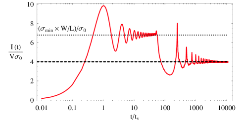
Figure 3: Total time dependent current $I(t)$ with geometric parameters $L\approx 25$ $n$m, $W\approx 106$ $n$m and applied voltage $V=8\times 10^{-4}$ Volt. Current is in units of $V\sigma_{0}$, where $\sigma_{0}=e^{2}/h$ is the quantum of conductance and time in units of $t_{v}=2.5\times 10^{-16}$ s. The dashed line represents the long-time conductance $\sigma_{2}/\sigma_{0}=4$ given by the Landauer formulaonipko2 , while the dotted line represents the combination $(\sigma_{\mathrm{min}}\times W/L)/\sigma_{0}=\pi/2\times W/L$.

For practical purposes we represent $H_{0}$ and $H(t)$ in a hybrid basis, in which the Hamiltonians of the isolated (equilibrium and biased) L and R reservoirs are diagonal in the set of states derived analytically in Ref.onipko, , while the Hamiltonian describing the C region remains represented in the basis $\{p,k_{y},i_{x}\}$. The enormous advantage of such choice is clarified in the following. Since we are interested in the dc conductance we set a small bias $V<<\hbar v_{F}/eW$. In this way we ensure that at long times a linear regime is established in which only the electrons right at the Dirac point (with $k_{y}=0$) contribute to the total current. This agrees with the Landauer formula, according to which only the states within the bias window contribute at the steady-state. On the other hand during the transient all transverse modes are excited and the sum in Eq.(4) must be computed including the complete set of $k_{y}$. Indeed we have checked numerically that in the limit $t\rightarrow\infty$ all currents $\bar{I}_{k_{y}}$, except the one with $k_{y}=0$, vanish. We have also observed that the damping time of $\bar{I}_{k_{y}>0}(t)$ goes like $k_{y}^{-1}$ and the calculation of the currents with small $k_{y}$ requires a very long propagation before the zero-current steady-state is approached. As a consequence very large values of $N_{r}$ are needed, making the computation in principle too demanding. Such numerical difficulty is, however, compensated by the fact that, after a transient time of order $L/v_{F}$, for $k_{y}$ close to the Dirac point only few low-energy states contribute to $\bar{I}_{k_{y}}(t)$. Therefore for any given $k_{y}>0$ we introduce an energy cutoff $\Lambda_{k_{y}}\approx 10\hbar v_{F}k_{y}$ in the reservoirs Hamiltonians and retain only the lead-eigenstates with transverese momentum $k_{y}$ and energy in the range $(-\Lambda_{k_{y}},\Lambda_{k_{y}})$. This allows us to deal with very long leads ($N_{r}>>1$) and can be explicitly implemented by using the analytic eigenstates of a rectangular graphenic macromoleculeonipko . The C region (which is the one where we calculate the current) is treated exactly within the original full basis $\{p,k_{y},i_{x}\}$, but the overall computational cost remains moderate.

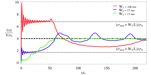
Figure 4: Short time transient current $I(t)$ for different ribbon widths $W_{1}=106$ $n$m, $W_{2}=27$ $n$m, $W_{3}=13$ $n$m. The rest of parameters, dotted/dashed lines and units are as in Fig.3.

In Fig.3 we show the time-dependent current $I(t)$ calculated for a nanoribbon of central length $L\approx 25$ $n$m ($N_{c}=100$) and width $W\approx 106$ $n$m ($N_{y}=250$) with an applied voltage $V=8\times 10^{-4}$ Volt and zero temperature. The very early transient regime ($t\lesssim\hbar/v\equiv t_{v}$) depends on the details with which the electric field $E$ has been switched-on (sudden in time in the present case). For $t_{v}\lesssim t\lesssim L/v_{F}$, however the time evolution only depends on the geometry of the device and on the potential profile. Within this time domain, if the ribbon is wide enough, the ballistic electron dynamics of the system probes only the bulk properties of graphene, since the particles do not have time to explore the reservoirs, where $E=0$. According to the Drude picture, the ballistic transport in bulk materials subjected to uniform electric fields produces a time-dependent conductance given by

$$\sigma(t)=\frac{\gamma t}{1+(\omega t)^{2}}\,,$$ (8)

where $\gamma$ is a constant proportional to the density of states. In ordinary solids the dc conductance ($\omega\rightarrow 0$) increases linearly in time up to the breakdown of the ballistic regime, in which one has to replace $t$ with the finite scattering time $\tau$. However in pure graphene the transport is ballistic up to very large length-scales of the order of micron and $\sigma$ can apparently diverge, producing a Drude peak. Nevertheless in undoped graphenic samples the density of states at the Fermi level vanishes, thus making the product $\gamma t$ constant at long times. This subtle compensation is at the origin of the finite minimal dc conductivity of 2D pure graphenelew and of the difficulties in constructing a suitable propagation scheme in finite width nanoribbons. In Fig.3 we see that $W\approx 100$ $n$m is enough to observe such compensation. The current $I(t)$, instead of increasing linearly in time, reaches a temporary plateau with average current $I_{1}$ which lasts till $t\approx L/v_{F}\approx 60t_{v}$. On the contrary in an ordinary system (e.g. in a 2D square lattice model) the current would be linear in time up to $L/v_{F}$, producing the well known Drude peak in the bulk limit $L,W\to\infty$ at fixed $E$. We would like to observe that the plateau at $I_{1}$ is reached via transient oscillations with frequency $2v/\hbar$lew . Interestingly such frequency is not displayed by any of the individual currents $\bar{I}_{k_{y}}(t)$, but appears only as a cumulative effect after the summation in Eq.(4) is performed. Therefore it is a a genuine bulk property and may be at the origin of the resonant effect predicted to occur in optical response of graphene right at $\omega=2v/\hbar$acgraphene .

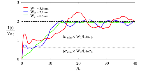
Figure 5: Short time transient current $I(t)$ for three different metallic armchair ribbons with open boundary conditions. The ribbon parameters are $L=5.5$ $n$m, $W_{1}=3.6$ $n$m, $W_{2}=2.1$ $n$m, $W_{3}=0.6$ $n$m and the applied bias is $V=0.03$ Volt. Units and dotted lines are as in Fig.3. The dashed line represents the long-time conductance $\sigma_{2}/\sigma_{0}=2$ given by the Landauer formulaperes ; onipko2 .

From the first plateau of $I(t)$ we can provide an independent evaluation of the minimal conductivity of graphene. According to its definition, the conductivity $\sigma_{1}$ of a bulk system subjected to a small constant electric field $E$ is given by the current density $J$ divided by $E$:

$$\sigma_{1}=\frac{J}{E}=\frac{I_{1}}{V}\frac{L}{W}\,.$$ (9)

By exploiting Eq.(9) it is seen that our data are consistent with the value $\sigma_{1}=\pi e^{2}/2h\equiv\sigma_{\mathrm{min}}$ with excellent precision, see Fig.3.

Further we have investigated the formation of the first plateau as a function of the ribbon width $W$. In Fig.4 we see that for narrow ribbons with $W\approx 10$ $n$m finite-size effects produce a drastic deviation from the ideal graphene bulk. The transient current does not show a temporary saturation, but grows with an approximate linear envelope (up to a time $\sim L/v_{F}$), in qualitative agreement with the Drude behavior given in Eq.(8).

At times larger than $\sim L/v_{F}$ the electrons start exploring the reservoirs, where the electric field is zero. At this point a standard dephasing mechanism sets in and the current tends to its true final steady-state. As discussed above, however, such value is reached after a very slow damping process, in which the current displays decaying oscillations with dominant frequency $\bar{\omega}=2\pi v_{F}/W$ (see Fig.3), $\hbar\bar{\omega}$ being the energy spacing between the transverse energy subbands of the ribbon. We have checked numerically that the asymptotic value $I_{2}$ agrees well with the Landauer formula and does not depend on $L$ and $W$, provided that $V<<\hbar v_{F}/eW$. Thus the conductance of the device is simply extracted as $\sigma_{2}=I_{2}/V$. Our numerical data provides $\sigma_{2}=4e^{2}/h$ with high numerical accuracy. This value is indeed twice the conductance of metallic nanoribbons, and this is due to the chosen periodic boundary conditionsonipko2 . Thus we have calculated $I(t)$ also in the case of open boundary conditions. Unfortunately, as discussed above, the lack of translational invariance along the transverse direction makes the computation much more demanding, and only system with small $L$ and $W$ can be studied within the present approach. In Fig.5 we show $I(t)$ for three different metallic armchair nanoribbons with open boundaries. It can be seen that already for $W\approx 2-4$ $n$m there is a tendency to form the universal first plateau leading to $\sigma_{\mathrm{min}}$, while for $W\lesssim 1$ $n$m the current $I(t)$ grows linearly in time until $t\approx L/v_{F}$. On the other hand at long times the current tends clearly to the Landauer value, consistent with $\sigma_{2}=2e^{2}/h$, independently on the aspect ratioperes ; onipko .

In summary we pointed out the subtle difficulties in constructing a reliable method to perform time-evolutions of finite width graphene nanoribbons and proposed an efficient numerical scheme to overcome them. We presented a real-time study of the transport properties of these systems in contact with virtual semi-infinite reservoirs in the linear regime. We have shown that for large enough undoped samples the time-dependent current displays two plateaus. From the first of these plateaus we can extract an independent measure of the minimal conductivity $\pi e^{2}/2$ of bulk graphene by resorting the aspect ratio $L/W$ of the device. The second plateau corresponds to reaching the steady-state and is independent of the geometry. Here the conductance is $2e^{2}/h$, which coincides with the Landauer result for metallic nanoribbons. To conclude we wish to point out that in presence of ac bias, the time-dependent conductivity can be used to obtain the optical conductivity $\sigma_{\mathrm{ac}}$ of graphene. It was shown experimentallyac1 and explained theoreticallyac2 that $\sigma_{\mathrm{ac}}$ is almost $\omega$-independent and equals $\sigma_{\mathrm{min}}$ with high accuracy over a wide range of frequencies. Remarkably to extract the universal value of $\sigma_{\mathrm{ac}}$ high frequency signals with $\omega\sim 1/t_{v}$ have been employedac1 . Therefore we believe that a real-time approach like to one presented here is needed to enlighten the crossover from the dc case to ultrafast scenarios in which the period of the ac signal is comparable with the intrinsic hopping time of the bulk system.

References

- (1) K. S. Novoselov et al., Science 306, 666 (2004).
- (2) K. S. Novoselov et al., Nature 438, 197 (2005). Y. Zhang et al., Nature 438, 201 (2005).
- (3) A. F. Young, P. Kim, Nature Phys. 5, 222 (2009); N. Stander et al., Phys. Rev. Lett. 102, 026807 (2009).
- (4) A. H. Castro Neto et al., Rev. Mod. Phys. 81, 109 (2009).
- (5) S.V. Morozov et al., Phys. Rev. Lett. 100, 016602 (2008).
- (6) G. Liang et al., IEEE Trans. Electron Devices 54, 657 (2007).
- (7) G. Gu et al., Appl. Phys. Lett. 90, 253507 (2007).
- (8) V. Ryzhii, M. Ryzhii, and T. Otsuji, J. Appl. Phys. 101, 024509 (2007).
- (9) F. Xia et al., Nature Nanotechnology, in press (2009).
- (10) K. Ziegler, Phys. Rev. Lett. 97, 266802 (2006); K. Ziegler, Phys. Rev. B 75, 233407 (2007).
- (11) N. M. R. Peres, F. Guinea, and A. H. Castro Neto, Phys. Rev. B 73, 125411 (2006).
- (12) J. Tworzydlo et al., Phys. Rev. Lett. 96, 246802 (2006).
- (13) L. A. Falkovsky and A. A. Varlamov, Eur. Phys. J. B 56, 281 (2007).
- (14) M. Lewkowicz and B. Rosenstein, Phys. Rev. Lett. 102, 106802 (2009).
- (15) Y. M. Blanter, and I. Martin, Phys. Rev. B 76, 155433 (2007).
- (16) M. I. Katsnelson, Eur. Phys. J. B 51, 157 (2006).
- (17) M. I. Katsnelson and F. Guinea, Phys. Rev. B 78, 075417 (2008).
- (18) A. Pecchia et al., Synthetic Metals 138, 89 (2003).
- (19) S. Roche et al., J. Phys.: Condens. Matter 19, 183203 (2007).
- (20) A. N. Andriotis, M. Menon, and D. Srivastava, J. Chem. Phys. 117, 2836 (2002).
- (21) E. Perfetto, G. Stefanucci, and M Cini, Phys. Rev. B 78, 155301 (2008).
- (22) L. Malysheva and A. Onipko, Phys. Rev. Lett. 100, 186806 (2008).
- (23) C. Zhang, L. Chen, and Z. S. Ma, Phys. Rev. B 77, 241402(R) (2008).
- (24) A. Onipko, Phys. Rev. B 78, 245412 (2008).
- (25) R. R. Nair et al., Science 320, 1308 (2008).
- (26) T. Stauber, N. M. R. Peres, and A. K. Geim, Phys. Rev. B 78, 085432 (2008).