Shock waves and compactons for
fifth-order nonlinear dispersion equations. II

Abstract.

The following first problem is posed: to justify that the standing shock wave

$$S_{-}(x)=-{\rm sign}\,x=\{-1\,\,\,\mbox{for}\,\,\,x<0,\,\,\,\,\,\,\,1\,\,\,\mbox{for}\,\,\,x>0\},$$

is a correct “entropy” solution of the Cauchy problem for the fifth-order degenerate nonlinear dispersion equations, NDEs (same as for the classic Euler one $u_{t}+uu_{x}=0$)

$$u_{t}=-(uu_{x})_{xxxx}\quad\mbox{and}\quad u_{t}=-(uu_{xxxx})_{x}\quad\mbox{in}\quad\mathbb{R}\times\mathbb{R}_{+}.$$

These two quasilinear degenerate PDEs are chosen as typical representatives, so other $(2m+1)$th-order NDEs of non-divergent form admit such shocks waves. As a related second problem, the opposite initial shock $S_{+}(x)=-S_{-}(x)={\rm sign}\,x$ is shown to be a non-entropy solution creating a rarefaction wave, which becomes $C^{\infty}$ for any $t>0$. Formation of shocks leads to nonuniqueness of any “entropy solutions”. Similar phenomena are studied for a fifth-order in time NDE $u_{ttttt}=(uu_{x})_{xxxx}$ in normal form. Other NDEs,

$$\mbox{e.g.,}\quad u_{t}=-(|u|u_{x})_{xxxx}+|u|u_{x}\quad\mbox{in}\quad\mathbb{R}\times\mathbb{R}_{+},$$

are shown to admit smooth compactons, as oscillatory travelling wave solutions with compact support. The well known nonnegative compactons, which appeared in various applications (first examples by Day, 1998, and Rosenau–Levy, 1999), are nonexistent in general and are not robust relative small perturbations of parameters of the PDE.

This is more extended and detailed version of the arXiv preprint [19]. Particularly, essential novelties are available in § 5.4, where a family of similarity extensions after blow-up was detected, which were mentioned but not found in [19, § 5].

1. Introduction: nonlinear dispersion PDEs, and main directions of study

1.1. Five main problems and layout: shocks, rarefaction waves, and compactons for fifth-order NDEs

Let us introduce our basic models, which are five fifth-order nonlinear dispersion equations (NDEs). These are ordered by numbers of derivatives inside and outside the quadratic differential operators involved on the right-hand sides:

(1.1) $$u_{t}=-uu_{xxxxx}\quad\quad\big{(}\mbox{NDE--$(5,0)$}\big{)},$$

(1.2) $$u_{t}=-(uu_{xxxx})_{x}\quad\big{(}\mbox{NDE--$(4,1)$}\big{)},$$

(1.3) $$u_{t}=-(uu_{xxx})_{xx}\quad\big{(}\mbox{NDE--$(3,2)$}\big{)},$$

(1.4) $$u_{t}=-(uu_{xx})_{xxx}\quad\big{(}\mbox{NDE--$(2,3)$}\big{)},$$

(1.5) $$u_{t}=-(uu_{x})_{xxxx}\quad\big{(}\mbox{NDE--$(1,4)$}\big{)}.$$

The only fully divergent operator is in the last NDE–$(1,4)$ that, being written as

(1.6) $$u_{t}=-(uu_{x})_{xxxx}\equiv-\frac{1}{2}\,(u^{2})_{xxxxx}\quad\big{(}\mbox{NDE--$(1,4)$ $=$ NDE--$(0,5)$}\big{)},$$

becomes also the NDE–$(0,5)$, or simply the NDE–5. This completes the list of such quasilinear degenerate PDEs under consideration.

The main feature of these degenerate odd-order PDEs is that they admit shock and rarefaction waves, similarly to the first-order conservation laws such as Euler’s equation

(1.7) $$u_{t}+uu_{x}=0\quad\mbox{in}\quad\mathbb{R}\times\mathbb{R}_{+},\quad u(x,0)=u_{0}(x)\quad\mbox{in}\quad\mathbb{R}.$$

Before explaining the physical significance of the NDEs and their role in general PDE theory, we pose four main problems for the above NDEs (the same as for (1.7)):

(I) Problem “Blow-up to $S_{-}$” (Section 2): to show that the shock of the shape $-{\rm sign}\,x$ can be obtained by blow-up limit from a smooth self-similar solution $u_{-}(x,t)$ of $(\ref{N50})$–$(\ref{N14})$ in $\mathbb{R}\times(0,T)$, i.e., the following holds:

(1.8) $$u_{-}(x,t)\to S_{-}(x)=-{\rm sign}\,x=\left\{\begin{matrix}\,\,\,\,1\,\,\,\mbox{\em for}\,\,\,x<0,\\ -1\,\,\,\mbox{\em for}\,\,\,x>0,\end{matrix}\right.\quad\mbox{\em as}\quad t\to T^{-}\quad\mbox{\em in \,\, $L^{1}_{\rm loc}(\mathbb{R})$}.$$

(II) The Riemann Problem $S_{+}$ $($RP$+)$ (Section 3): to show that the initial shock

(1.9) $$S_{+}(x)={\rm sign}\,x=\left\{\begin{matrix}-1\,\,\,\mbox{\em for}\,\,\,x<0,\\ \,\,\,\,1\,\,\,\mbox{\em for}\,\,\,x>0,\end{matrix}\right.$$

for NDEs $(\ref{N50})$–$(\ref{N14})$ generates a “rarefaction wave”, which is $C^{\infty}$-smooth for $t>0$.

(III) The Riemann Problem $S_{-}$ $($RP$-)$ (Section 4): introducing a “$\delta$-entropy test” (smoothing of discontinuous solutions at shocks via a “$\delta$-deformation”), to show that

(1.10) $$S_{-}(x)\,\,\,\mbox{\em is an ``$\delta$-entropy" shock wave, and}\,\,\,S_{+}(x)\,\,\,\mbox{\em is not}.$$

(IV) Problem: nonuniqueness/entropy (Section 5): to show that a single point “gradient catastrophe” for the NDE $(\ref{N14})$ leads to the principal nonuniqueness of a shock wave extension after singularity. This also suggests nonexistence of any proper entropy mechanism for choosing any “right” solution after single point blow-up.

In Section 6, we discuss these problems in application to other NDEs including the following rather unusual one:

(1.11) $$u_{ttttt}=(uu_{x})_{xxxx},$$

which indeed can be reduced to a first-order system that, nevertheless, is not hyperbolic, so that modern advanced theory of 1D hyperbolic systems (see e.g., Bressan [1] or Dafermos [10]) does not apply. The main convenient mathematical feature of (1.11) is that it is in the normal form, so it obeys the Cauchy–Kovalevskaya theorem that guarantees local existence of a unique analytic solution and makes easier application of our $\delta$-entropy (smoothing) test. Regardless this, (1.11) is shown to create in finite time shocks of the type $S_{-}(x)$ in (1.8) and rarefaction waves for other discontinuous data $\sim S_{+}(x)$ in (1.9).

Finally, we consider the last:

(V) Problem “Oscillatory Smooth Compactons” (Section 7): to show that the perturbed version of the NDE $(\ref{N14})$, as a typical example,

(1.12) $$u_{t}=-(|u|u_{x})_{xxxx}+|u|u_{x}\quad\mbox{in}\quad\mathbb{R}\times\mathbb{R}_{+},$$

admits compactly supported travelling wave (TW) solutions of changing sign near finite interfaces. Equation (1.12) is written for solutions with infinitely many sign changes, by replacing $u^{2}$ by the monotone function $|u|u$.

Nonnegative compact structures have been known since beginning of the 1990s as compactons (Rosenau–Hyman, 1993, [47]). We show that more standard in literature nonnegative compactons of fifth-order NDEs such as (1.12) are nonexistent in general, and, moreover, these are not robust (not “structurally stable”), i.e., do not exhibit continuous dependence upon the parameters of PDEs (say, arbitrarily small perturbations of nonlinearities).

1.2. A link to classic entropy shocks for conservation laws

Indeed, the above problems (I)–(III) are classic for entropy theory of 1D conservation laws from the 1950s. It is well recognized that shock waves first appeared in gas dynamics that led to mathematical theory of entropy solutions of the first-order conservation laws and Euler’s equation (1.7) as a key representative. The entropy theory for PDEs such as (1.7), with arbitrary measurable initial data $u_{0}$, was created by Oleinik [36, 37] and Kruzhkov [31] (analogous scalar equations in $\mathbb{R}^{N}$) in the 1950–60s; see details on the history, main results, and modern developments in the well-known monographs [1, 10, 50]. Note that first analysis of the formation of shocks for (1.7) was performed by Riemann in 1858 [42]; see further details and the history in [3]. It is worth mentioning that the implicitly given solution $u=u(x,t)$ of the Cauchy problem (1.7), via the characteristic formula

$$u=u_{0}(x-u\,t),$$

containing the key wave “overturning” effect, was obtained earlier by Poisson in 1808 [39]; see [40].

According to entropy theory for conservation laws such as (1.7), it is well-known that (1.10) holds. This means that

(1.13) $$u_{-}(x,t)\equiv S_{-}(x)=-{\rm sign}\,x$$

is the unique entropy solution of the PDE (1.7) with the same initial data $S_{-}(x)$. On the contrary, taking $S_{+}$-type initial data (1.9) in the Cauchy problem (1.7) yields the continuous rarefaction wave with a simple similarity piece-wise linear structure,

(1.14) $$u_{0}(x)=S_{+}(x)={\rm sign}\,x\,\,\,\Longrightarrow\,\,\,u_{+}(x,t)=g(\frac{x}{t})=\left\{\begin{matrix}-1\quad\mbox{for}\,\,\,x<-t,\cr\,\,\,\frac{x}{t}\quad\mbox{for}\,\,\,|x|<t,\cr 1\quad\,\mbox{for}\,\,\,x>t.\end{matrix}\right.$$

Our first goal is to justify the same conclusions for the fifth-order NDEs, where, of course, the rarefaction wave in the RP$+$ is supposed to be different from that in (1.14).

We now return to main applications of the NDEs.

1.3. NDEs from theory of integrable PDEs and water waves

Talking about odd-order PDEs under consideration, these naturally appear in classic theory of integrable PDEs from shallow water applications, beginning with the KdV equation,

(1.15) $$u_{t}+uu_{x}=u_{xxx},$$

the fifth-order KdV equation,

$$u_{t}+u_{xxxxx}+30\,u^{2}u_{x}+20\,u_{x}u_{xx}+10\,uu_{xxx}=0,$$

and others. These are semilinear dispersion equations, which being endowed with smooth semigroups (groups), generate smooth flows, so discontinuous weak solutions are unlikely, though strong oscillatory behaviour of solutions is typical; see references in [24, Ch. 4].

The situation is changed for the quasilinear case. In particular, consider the quasilinear Harry Dym equation

(1.16) $$u_{t}=u^{3}u_{xxx}\,,$$

which is one of the most exotic integrable soliton equations; see [24, § 4.7] for survey and references therein. Here, (1.16) indeed belongs to the NDE family, though it seems proper semigroups of its discontinuous solutions (if any) have never been examined. On the other hand, moving blow-up singularities and other types of complex singularities of the modified Harry Dym equation,

$$u_{t}=u^{3}u_{xxx}-u_{x}-\frac{1}{2}\,u^{3},$$

have been described in [6] by delicate asymptotic expansion techniques.

In addition, integrable equation theory produced various hierarchies of quasilinear higher-order NDEs, such as the fifth-order Kawamoto equation [30], as a typical example

(1.17) $$u_{t}=u^{5}u_{xxxxx}+5\,u^{4}u_{x}u_{xxxx}+10\,u^{5}u_{xx}u_{xxx}.$$

We can enlarge this list talking about possible quasilinear extensions of the integrable Lax’s seventh-order KdV equation

$$u_{t}+[35u^{4}+70(u^{2}u_{xx}+u(u_{x})^{2})+7(2uu_{xxxx}+3(u_{xx})^{2}+4u_{x}u_{xxx})+u_{xxxxxx}]_{x}=0,$$

and the seventh-order Sawada–Kotara equation

$$u_{t}+[63u^{4}+63(2u^{2}u_{xx}+u(u_{x})^{2})+21(uu_{xxxx}+(u_{xx})^{2}+u_{x}u_{xxx})+u_{xxxxxx}]_{x}=0;$$

see references in [24, p. 234].

The modern mathematical theory of odd-order quasilinear PDEs is partially originated and continues to be strongly connected with the class of integrable equations. Special advantages of integrability by using the inverse scattering transform method, Lax pairs, Liouville transformations, and other explicit algebraic manipulations have made it possible to create a rather complete theory for some of these difficult quasilinear PDEs. Nowadays, well-developed theory and most of rigorous results on existence, uniqueness, and various singularity and non-differentiability properties are associated with NDE-type integrable models such as Fuchssteiner–Fokas–Camassa–Holm (FFCH) equation

(1.18) $$(I-D_{x}^{2})u_{t}=-3uu_{x}+2u_{x}u_{xx}+uu_{xxx}\equiv-(I-D_{x}^{2})(uu_{x})-\big{[}u^{2}+\frac{1}{2}\,(u_{x})^{2}\big{]}.$$

Equation (1.18) is an asymptotic model describing the wave dynamics at the free surface of fluids under gravity. It is derived from Euler equations for inviscid fluids under the long wave asymptotics of shallow water behaviour (where the function $u$ is the height of the water above a flat bottom). Applying to (1.18) the integral operator $(I-D_{x}^{2})^{-1}$ with the $L^{2}$-kernel $\omega(s)=\frac{1}{2}\,{\mathrm{e}}^{-|s|}>0$, reduces it, for a class of solutions, to the conservation law (1.7) with a compact first-order perturbation,

(1.19) $$u_{t}+uu_{x}=-\big{[}\omega*\big{(}u^{2}+\frac{1}{2}(u_{x})^{2}\big{)}\big{]}_{x}.$$

Almost all mathematical results (including entropy inequalities and Oleinik’s condition (E)) have been obtained by using this integral representation of the FFCH equation; see the long list of references given in [24, p. 232].

There is another integrable PDE from the family with third-order quadratic operators,

(1.20) $$u_{t}-u_{xxt}=\alpha uu_{x}+\beta u_{x}u_{xx}+uu_{xxx}\quad(\alpha,\,\beta\in\mathbb{R}),$$

where $\alpha=-3$ and $\beta=2$ yields the FFCH equation (1.18). This is the Degasperis–Procesi (DP) equation for another choice $\alpha=-4$ and $\beta=3$:

(1.21) $$u_{t}-u_{xxt}=-4uu_{x}+3u_{x}u_{xx}+uu_{xxx},\quad\mbox{or}\quad u_{t}+uu_{x}=-\big{[}\omega*\big{(}\frac{3}{2}\,u^{2}\big{)}\big{]}_{x}.$$

On existence, uniqueness (of entropy solutions in $L^{1}\cap BV$), parabolic $\varepsilon$-regularization, Oleinik’s entropy estimate, and generalized PDEs, see [5].

Note that, since the non-local term in the DP equation (1.21) does not contain $u_{x}$, the differential properties of its solutions are distinct from those for the FFCH one (1.19). Namely, the solutions are less regular, and (1.21) admits shock waves, e.g., of the form

$$u_{\rm shock}(x,t)=-\frac{1}{t}\,{\rm sign}\,x\,{\mathrm{e}}^{-|x|},$$

with rather standard (induced by (1.7)) but more involved entropy theory; see [32, 14].

Besides (1.18) and (1.21), the family (1.20) does not contain other integrable entries. A list of more applied papers related to various NDEs is also available in [24, Ch. 4].

1.4. NDEs from compacton theory

Other important applications of odd-order PDEs are associated with compacton phenomena for more general non-integrable models. For instance, the Rosenau–Hyman (RH) equation

(1.22) $$u_{t}=(u^{2})_{xxx}+(u^{2})_{x}$$

has special important applications as a widely used model of the effects of nonlinear dispersion in the pattern formation in liquid drops [47]. It is the $K(2,2)$ equation from the general $K(m,n)$ family of the following NDEs:

(1.23) $$u_{t}=(u^{n})_{xxx}+(u^{m})_{x}\quad(u\geq 0),$$

that describe phenomena of compact pattern formation, [43, 44]. Such PDEs also appear in curve motion and shortening flows [46]. Similar to well-known parabolic models of the porous medium type, the $K(m,n)$ equation (1.23) with $n>1$ is degenerate at $u=0$, and therefore may exhibit finite speed of propagation and admit solutions with finite interfaces. The crucial advantage of the RH equation (1.22) is that it possesses explicit moving compactly supported soliton-type solutions, called compactons [47, 43], which are travelling wave (TW) solutions to be discussed for the PDEs under consideration.

Various families of quasilinear third-order KdV-type equations can be found in [4], where further references concerning such PDEs and their exact solutions are given. Higher-order generalized KdV equations are of increasing interest; see e.g., the quintic KdV equation in [28], and also [55], where the seventh-order PDEs are studied.

More general $B(m,k)$ equations,

$$u_{t}+a(u^{m})_{x}=\mu(u^{k})_{xxx},$$

which coincide with the $K(m,k)$ after scaling, also admit simple semi-compacton solutions [48]. The same is true for the $Kq(m,\omega)$ nonlinear dispersion equation (another nonlinear extension of the KdV) [43]

$$u_{t}+(u^{m})_{x}+[u^{1-\omega}(u^{\omega}u_{x})_{x}]_{x}=0.$$

Setting $m=2$ and $\omega=\frac{1}{2}$ yields a typical quadratic PDE

(1.24) $${\bf B}(u)\equiv u_{t}+(u^{2})_{x}+uu_{xxx}+2u_{x}u_{xx}=0.$$

It is curious that (1.24) admits an extended compacton-like dynamics on a standard trigonometric-exponential subspaces, on which

(1.25) $$u(x,t)=C_{0}(t)+C_{1}(t)\cos\lambda x+C_{2}(t)\sin\lambda x\in W_{3}={\rm Span}\{1,\cos\lambda x,\sin\lambda x\},$$

where $\lambda=\sqrt{\frac{2}{3}}$. This subspace is invariant under the quadratic operator ${\bf B}$ in the usual sense that ${\bf B}(W_{3})\subseteq W_{3}$. Therefore substituting (1.25) into the PDE 1.24) yields for the expansion coefficients on $W_{3}$ $\{C_{0},C_{1},C_{2}\}$ a 3D nonlinear dynamical system; see further such examples of exact solutions of NDEs on invariant subspaces in [24, Ch. 4].

Combining the $K(m,n)$ and $B(m,k)$ equations gives the dispersive-dissipativity entity $DD(k,m,n)$ [45]

$$u_{t}+a(u^{m})_{x}+(u^{n})_{xxx}=\mu(u^{k})_{xx},$$

which can also admit solutions on invariant subspaces for some values of parameters.

For the fifth-order NDEs, such as

(1.26) $$u_{t}=\alpha(u^{2})_{xxxxx}+\beta(u^{2})_{xxx}+\gamma(u^{2})_{x}\quad\mbox{in}\,\,\,\mathbb{R}\times\mathbb{R}_{+},$$

compacton solutions were first constructed in [11], where the more general $K(m,n,p)$ family of PDEs,

$$u_{t}+\beta_{1}(u^{m})_{x}+\beta_{2}(u^{n})_{xxx}+\beta_{3}D_{x}^{5}(u^{p})=0,$$

with $m,\,n,\,p>1$, was introduced. Some of these equations will be treated later on. Equation (1.26) is also associated with the family $Q(l,m,n)$ of more general quintic evolution PDEs with nonlinear dispersion,

(1.27) $$u_{t}+a(u^{m+1})_{x}+\omega\bigl{[}u(u^{n})_{xx}\bigr{]}_{x}+\delta\bigl{[}u(u^{l})_{xxxx}\bigr{]}_{x}=0,$$

possessing multi-hump, compact solitary solutions [49].

Concerning higher-order in time quasilinear PDEs, let us mention a generalization of the combined dissipative double-dispersive (CDDD) equation (see, e.g., [41])

(1.28) $$u_{tt}=\alpha u_{xxxx}+\beta u_{xxtt}+\gamma(u^{2})_{xxxxt}+\delta(u^{2})_{xxt}+\varepsilon(u^{2})_{t},$$

and also the nonlinear modified dispersive Klein–Gordon equation ($mKG(1,n,k)$),

(1.29) $$u_{tt}+a(u^{n})_{xx}+b(u^{k})_{xxxx}=0,\quad n,k>1\quad(u\geq 0);$$

see some exact TW solutions in [29]. For $b>0$, (1.29) is of hyperbolic (or Boussinesq) type in the class of nonnegative solutions. We also mention related 2D dispersive Boussinesq equations denoted by $B(m,n,k,p)$ [54],

$$(u^{m})_{tt}+\alpha(u^{n})_{xx}+\beta(u^{k})_{xxxx}+\gamma(u^{p})_{yyyy}=0\quad\mbox{in}\quad\mathbb{R}^{2}\times\mathbb{R}.$$

See [24, Ch. 4-6] for more references and examples of exact solutions on invariant subspaces of NDEs of various types and orders.

1.5. On canonical third-order NDEs

Until recently, quite a little was known about proper mathematics concerning discontinuous solutions, rarefaction waves, and “entropy-like” approaches, even for the simplest third-order NDEs such as (1.22) or (see [23, 18])

(1.30) $$u_{t}=(uu_{x})_{xx}.$$

However, the smoothing results for sufficiently regular solutions of linear and nonlinear third-order PDEs are well know from the 1980-90s. For instance, infinite smoothing results were proved in [7] (see also [27]) for the general linear equation

(1.31) $$u_{t}+a(x,t)u_{xxx}=0\quad(a(x,t)\geq c>0),$$

and in [8] for the corresponding fully nonlinear PDE

(1.32) $$u_{t}+f(u_{xxx},u_{xx},u_{x},u,x,t)=0\quad\big{(}\,f_{u_{xxx}}\geq c>0\,\big{)};$$

see also [2] for semilinear equations. Namely, for a class of such equations, it is shown that, for data with minimal regularity and sufficient (say, exponential) decay at infinity, there exists a unique solution $u(x,t)\in C^{\infty}_{x}$ for small $t>0$. Similar smoothing local in time results for unique solutions are available for equations in $\mathbb{R}^{2}$,

(1.33) $$u_{t}+f(D^{3}u,D^{2}u,Du,u,x,y,t)=0;$$

see [33] and further references therein.

These smoothing results have been used in [18] for developing a kind of a $\delta$-entropy test for discontinuous solutions by using techniques of smooth deformations. We will follow these ideas applied now to shock and compacton solutions of higher-order NDEs and others.

2. (I) Problem “Blow-up”: existence of shock $S_{-}$ similarity solutions

We now show that Problem (I) on blowing up to the shock $S_{-}(x)$ can be solved in a unified manner by constructing self-similar solutions. As often happens in nonlinear evolution PDEs, the refined structure of such bounded and generic shocks is described in a scaling-invariant manner.

2.1. Finite time blow-up formation of the shock wave $S_{-}(x)$

One can see that all five NDEs (1.1)–(1.5) admit the following similarity substitution:

(2.1) $$u_{-}(x,t)=g(z),\quad z=x/(-t)^{\frac{1}{5}}\quad(t<0),$$

where, by translation, the blow-up time in reduces to $T=0$. Substituting (2.1) into the NDEs yields for $g$ the following ODEs in $\mathbb{R}$, respectively:

(2.2) $$gg^{(5)}=-\textstyle{\frac{1}{5}}\,g^{\prime}z,$$

(2.3) $$(gg^{(4)})^{\prime}=-\textstyle{\frac{1}{5}}\,g^{\prime}z,$$

(2.4) $$(gg^{\prime\prime\prime})^{\prime\prime}=-\textstyle{\frac{1}{5}}\,g^{\prime}z,$$

(2.5) $$(gg^{\prime\prime})^{\prime\prime\prime}=-\textstyle{\frac{1}{5}}\,g^{\prime}z,$$

(2.6) $$(gg^{\prime})^{(4)}=-\textstyle{\frac{1}{5}}\,g^{\prime}z,$$

with the following conditions at infinity for the shocks $S_{-}$:

(2.7) $$g(\mp\infty)=\pm 1.$$

In view of the symmetry of the ODEs,

(2.8) $$\left\{\begin{matrix}g\mapsto-g,\\ z\mapsto-z,\end{matrix}\right.$$

it suffices to get odd solutions for $z<0$ posing anti-symmetry conditions at the origin,

(2.9) $$g(0)=g^{\prime\prime}(0)=g^{(4)}(0)=0.$$

2.2. Shock similarity profiles exist and are unique: numerical results

Before performing a rigorous approach to Problem (I), it is convenient and inspiring to check whether the shock similarity profiles $g(z)$ announced in (2.1) actually exist and are unique for each of the ODEs (2.2)–(2.6). This is done by numerical methods that supply us with positive and convincing conclusions. Moreover, these numerics clarify some crucial properties of profiles, which will determine the actual strategy of rigorous study.

A typical structure of this shock similarity profile $g(z)$ satisfying (2.2), (2.9) is shown in Figure 1. As a key feature, we observe a highly oscillatory behaviour of $g(z)$ about $\pm 1$ as $z\to\mp\infty$, that can essentially affect the metric of the announced convergence (1.8). Therefore, we will need to describe this oscillatory behaviour in detail. In Figure 2, we show the same profile $g(z)$ for smaller $z$. It is crucial that, in all numerical experiments, we obtained the same profile that indicates that it is the unique solution of (2.2), (2.9).

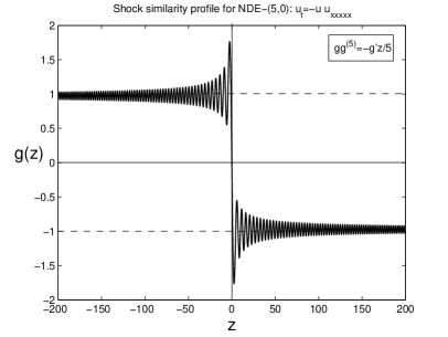
Figure 1. The shock similarity profile $g(z)$ as the unique solution of the problem (2.2), (2.9); $z\in[-200,200]$.

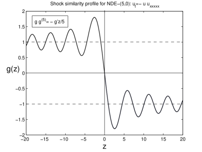
Figure 2. The shock similarity profile $g(z)$ as the unique solution of the problem (2.2), (2.9); $z\in[-20,20]$.

Figure 3(a)–(d) show the shock similarity profiles for the rest of NDEs (1.2)–(1.5). They differ from each other rather slightly.

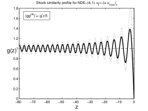
(a) equation (2.3)

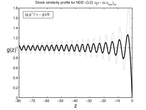
(b) equation (2.4)

(c) equation (2.5)

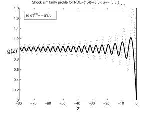
(d) equation (2.6)

Figure 3. Shock similarity profiles as solutions of (2.3)–(2.6), (2.9) respectively. For comparison, dotted lines denote the profile from Figures 1 and 2.

Remark: on regularization in numerical methods. For the fifth-order NDEs, this and further numerical constructions are performed by MatLab by using the bvp4c solver. Typically, we take the relative and absolute tolerances

(2.10) $${\rm Tols}=10^{-4}.$$

Instead of the degenerate ODE (2.2) (or others), we solve the regularized equation

(2.11) $$g^{(5)}=-\frac{{\rm sign}\,g}{\sqrt{\nu^{2}+g^{2}}}\,\big{(}\frac{1}{5}\,g^{\prime}z\big{)},\quad\mbox{with the regularization parameter $\nu=10^{-4}$},$$

where the choice of small $\nu$ is coherent with the tolerances in (2.10). Sometimes, we will need to use the enhanced parameters ${\rm Tols}=\nu=10^{-7}$ or even $\sim 10^{-9}$.

2.3. Justification of oscillatory behaviour about equilibria $\pm 1$ and other asymptotics

Thus, the shock profiles $g(z)$ are oscillatory about $+1$ as $z\to-\infty$. In order to describe these oscillations in detail, we linearize all the ODEs (2.2)–(2.6) about the regular equilibrium $g(z)\equiv 1$ by setting $g=1+\hat{g}$ to get the linear ODE

(2.12) $${\bf B}_{5}^{*}\,\hat{g}\equiv-\hat{g}^{(5)}-\frac{1}{5}\,\hat{g}^{\prime}z=0.$$

Note that this equation reminds us of that for the rescaled kernel $F(z)$ of the fundamental solution of the corresponding linear dispersion equation,

(2.13) $$u_{t}=-u_{xxxxx}\quad\mbox{in}\,\,\,\,\mathbb{R}\times\mathbb{R}_{+}.$$

The fundamental solution of the corresponding linear operator $\frac{\partial}{\partial t}+D_{x}^{5}$ in (2.13) has the standard similarity form

(2.14) $$b(x,t)=t^{-\frac{1}{5}}F(y),\,\,\,\,\mbox{with}\,\,\,\,y=x/{t^{1/5}},$$

where $F(y)$ is a unique solution of the ODE problem

(2.15) $${\bf B}_{5}F\equiv-F^{(5)}+\frac{1}{5}\,(Fy)^{\prime}=0\,\,\mbox{in}\,\,\mathbb{R},\,\,\,\int F=1,\quad\mbox{or $F^{(4)}=\frac{1}{5}\,Fy$ on integration}.$$

However, the operator ${\bf B}_{5}$ in (2.15) is not identical to that in (2.12). Moreover, this ${\bf B}^{*}_{5}$ is adjoint to ${\bf B}_{5}$ in some indefinite metric and both the operators possess countable families of eigenfunctions, which particularly are generalized Hermite polynomials for ${\bf B}_{5}^{*}$. We will not use this Hermitian spectral theory later on, so refer to [17, § 9] and [20, § 8.2] for further results and applications.

Let us return to the linearized ODE (2.12). Looking for possible asymptotics as $z\to-\infty$ yields the following exponential ones with the characteristic equation:

(2.16) $$\hat{g}(z)\sim{\mathrm{e}}^{a|z|^{5/4}}\quad\Longrightarrow\quad a^{4}=\frac{4^{4}}{5^{5}}.$$

Finally, choosing the purely imaginary root of the algebraic equation in (2.16) with ${\rm Re}\,a=0$ gives a refined WKBJ-type asymptotics of solutions of (2.2):

(2.17) $$g(z)=1+|z|^{-\frac{5}{8}}\bigl{[}A\sin\bigl{(}{a_{0}}|z|^{\frac{5}{4}}\bigr{)}+B\cos\bigl{(}{a_{0}}|z|^{\frac{5}{4}}\bigr{)}\bigr{]}+...\,\,\,\mbox{as}\,\,\,z\to-\infty,$$

where $A$ and $B$ are some real constants satisfying $A^{2}+B^{2}\neq 0$.

The asymptotic behaviour (2.17) implies two important conclusions:

Proposition 2.1.

The shock wave profiles $g(z)$ solving $(\ref{1E})$–$(\ref{5E})$, $(\ref{2.2})$ satisfy: (i)

(2.18) $$\quad g(z)-1\not\in L^{1}(\mathbb{R}_{-}),\quad\mbox{and}$$

(ii) the total variation of $g(z)$ $($and hence of $u_{-}(x,t)$ for any $t<0)$ is infinite.

Proof. Setting $|z|^{\frac{5}{4}}=v$ in the integrals below yields by (2.17):

(2.19) $$\begin{matrix}\mbox{${\rm(i)}\quad\int\limits_{-\infty}|g(z)-1|\,{\mathrm{d}}z\sim\int\limits^{\infty}\frac{|\cos z^{\frac{5}{4}}|}{z^{5/8}}\,{\mathrm{d}}z\sim\int\limits^{\infty}\frac{|\cos v|}{v^{7/10}}\,{\mathrm{d}}v=\infty;\quad\mbox{and}\qquad\qquad$}\vskip 3.0pt plus 1.0pt minus 1.0pt\vskip 3.0pt plus 1.0pt minus 1.0pt\\ {\rm(ii)}\quad\mbox{$|g(\cdot)|_{\rm Tot.Var.}=\int\limits_{-\infty}^{+\infty}|g^{\prime}(z)|\,{\mathrm{d}}z\sim\int\limits^{\infty}\frac{|\cos z^{\frac{5}{4}}|}{z^{3/8}}\,{\mathrm{d}}z\sim\int\limits^{\infty}\frac{|\cos v|}{\sqrt{v}}\,{\mathrm{d}}v=\infty.\qed\qquad\qquad$}\end{matrix}$$

This is in striking contrast with the case of conservation laws (1.7), where finite total variation approaches and Helly’s second theorem (compact embedding of sets of bounded functions of bounded total variations into $L^{\infty}$) used to be key; see Oleinik’s pioneering approach [36]. In view of the presented properties of the similarity shock profile $g(z)$, the convergence in (1.8) takes place for any $x\in\mathbb{R}$, uniformly in $\mathbb{R}\setminus(-\mu,\mu)$, $\mu>0$ small, and in $L^{p}_{\rm loc}(\mathbb{R})$ for $p\in[1,\infty)$, that, for convenience, we fix in the following:

Proposition 2.2.

For the shock similarity profile $g(z)$ the convergence $(\ref{con32})$ with $T=0$:

(i) does not hold in $L^{1}(\mathbb{R})$, and

(ii) does hold in $L^{1}_{\rm loc}(\mathbb{R})$, and moreover, for any fixed finite $l>0$,

(2.20) $$\|u_{-}(\cdot,t)-S_{-}(\cdot)\|_{L^{1}(-l,l)}=O((-t)^{\frac{1}{8}})\to 0\quad\mbox{as}\quad t\to 0^{-}.$$

Proof of (2.20) is the same as in (2.19) with a finite interval of integration: for $l=1$,

$$\|\cdot\|_{L^{1}(-1,1)}\sim(-t)^{\frac{1}{5}}\int\limits^{(-t)^{-1/5}}z^{-\frac{5}{8}}|\cos z^{\frac{5}{4}}|\,{\mathrm{d}}z\sim(-t)^{\frac{1}{5}}\int\limits^{(-t)^{-1/4}}v^{-\frac{7}{10}}|\cos v|\,{\mathrm{d}}v\sim(-t)^{\frac{1}{8}}.\qed$$

Finally, note that each $g(z)$ has a regular asymptotic expansion near the origin. For instance, for the first ODE (2.2), there exist solutions such that

(2.21) $$g(z)=Cz+Dz^{3}-\frac{1}{600}\,z^{5}+\frac{D}{6300C}\,z^{7}+...\,,$$

where $C<0$ and $D\in\mathbb{R}$ are some constants. The local uniqueness of such asymptotics is traced out by using Banach’s Contraction Principle applied to the equivalent integral equation in the metric of $C(-\mu,\mu)$, with $\mu>0$ small. Moreover, it can be shown that (2.21) is the expansion of an analytic function. Other ODEs admit similar local representations of solutions.

We now need the following scaling invariance of the ODEs (2.2)–(2.6): if $g_{1}(z)$ is a solution, then

(2.22) $$g_{a}(z)=a^{5}g_{1}\big{(}\frac{z}{a}\big{)}\quad\mbox{is a solution for any $a\not=0$}.$$

2.4. Existence of a shock similarity profile

Using the asymptotics derived above, we now in a position to prove the following:

Proposition 2.3.

The problem $(\ref{2.2})$, $(\ref{2.4})$ for ODEs $(\ref{1E})$–$(\ref{5E})$ admits a solution $g(z)$, which is an odd analytic function.

Uniqueness for such higher-order ODEs is a more difficult problem, which is not studied here, though it has been seen numerically. Moreover, there are some analogous results. We refer to the paper [25] (to be used later on), where uniqueness of a fourth-order semilinear ODE was established by an improved shooting argument.

Notice another difficult aspect of the problem. Figures 1–3 above, which were obtained by careful numerics, clearly convince that the positivity holds:

(2.23) $$g(z)>0\quad\mbox{for}\quad z<0,$$

which is also difficult to prove rigorously; see further comments below. Actually, (2.23) is not that important for the key convergence (1.8), since possible sign changes (if any) disappear in the limit as $t\to T^{-}$. It seems that nothing prevents existence of some ODEs from the family (2.2)–(2.6), with different nonlinearities, for which the shock profiles can change sign for $z<0$.

Proof. As above, we consider the first ODE (2.2) only. We use a shooting argument using the 2D bundle of asymptotics (2.21). By scaling (2.22), we put $C=-1$, so, actually, we deal with the one-parameter shooting problem with the 1D family of orbits satisfying

(2.24) $$g(z;D)=-z+D\,z^{3}-\frac{1}{600}\,z^{5}-\frac{D}{6300}\,z^{7}+...\,,\quad D\in\mathbb{R}.$$

It is not hard to check that, besides stabilization to unstable constant equilibria,

(2.25) $$g(z)\to C_{-}>0\quad\mbox{as}\quad z\to-\infty,$$

the ODE (2.3) admits an unbounded stable behaviour given by

(2.26) $$g(z)\sim g_{*}(z)=-\frac{1}{120}\,z^{5}\to+\infty\quad\mbox{as}\quad z\to-\infty.$$

The overall asymptotic bundle about the exact solution $g_{*}(z)$ is obtained by linearization: as $z\to-\infty$,

(2.27) $$g(z)=g_{*}(z)+Y(z)\quad\Longrightarrow\quad g_{*}Y^{(5)}=-\frac{1}{5}Y^{\prime}z+...\,\,\,\mbox{or}\,\,\,z^{5}Y^{(5)}=24Y^{\prime}z+...\,.$$

This is Euler’s type homogeneous equation with the characteristic equation

(2.28) $$Y(z)=z^{m}\quad\Longrightarrow\quad m_{1}=0\,\,(Y_{2}(z)\equiv 1)\,\,\,\mbox{or}\,\,\,(m-1)(m-2)(m-3)(m-4)=24.$$

This yields another $m_{2}=0$ (hence there exists $Y_{2}(z)=\ln|z|$), $m_{3}=5$ (not suitable), and a proper single complex root with ${\rm Re}\,m=\frac{5}{2}<5$ yielding oscillatory $Y_{3,4}(z)$. Thus:

(2.29) as $$z\to-\infty g_{*}(z)=-\frac{1}{120}\,z^{5}$$, there exists a 4D asymptotic bundle about .

Therefore, at $z=-\infty$, we are given a 2D bundle of proper solutions (2.17), as well as a 4D fast growing profiles from (2.29). This determines the strategy of the 1D shooting via the $D$-family (2.24):

(i) obviously, for all $D\ll-1$, we have that $g(z;D)>0$ is monotone decreasing and approaches the stable behaviour (2.26), (2.29), and

(ii) on the contrary, for all $D\gg 1$, $g(z;D)$ gets non-monotone and has a zero at some finite $z_{0}=z_{0}(D)<0$, satisfying $z_{0}(D)\to 0^{-}$ as $D\to+\infty$, and eventually approaches the bundle in (2.29), but in an essentially non-monotone way.

It follows from different and opposite “topologies” of the behaviour announced in (i) and (ii) that there exists a constant $D_{0}$ such that $g(z;D_{0})$ does not belong to those two sets of orbits (both are open) and hence does not approach $g_{*}(z)$ as $z\to-\infty$ at all. This is precisely the necessary shock similarity profile. ∎

This 1D shooting approach is explained in Figure 4 obtained numerically, where

(2.30) $$D_{0}=0.069192424...\,.$$

It seems that as $D\to D_{0}^{+}$, the zero of $g(z;D)$ must disappear at infinity, i.e.,

(2.31) $$z_{0}(D)\to-\infty\quad\mbox{as}\quad D\to D_{0}^{+},$$

and this actually happens as Figure 4 shows. Then this would justify the positivity (2.23). Unfortunately, in general (i.e., for similar ODEs with different sufficiently arbitrary nonlinearities), this is not true, i.e., cannot be guaranteed by a topological argument. So that the actual operator structure of the ODEs should be involved in the study, so, theoretically, the positivity is difficult to guarantee in general. Note again that, if the shock similarity profile $g(z)$ had a few zeros for $z<0$, this would not affect the crucial convergence property such as (1.8).

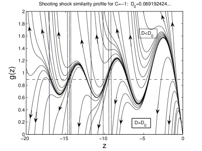
Figure 4. Shooting the shock similarity profile $g(z)$ via the family (2.24); $D_{0}=0.069192424...\,$.

2.5. Self-similar formation of other shocks

NDE–$(1,4)$. Let us first briefly consider the last ODE (2.6) for the fully divergent NDE (1.5). Similarly, by the same arguments, we show that, according to (2.1), there exist other non-symmetric shocks as non-symmetric step-like functions, so that, as $t\to 0^{-}$,

(2.32) $$u_{-}(x,t)\to\left\{\begin{matrix}C_{-}>0\,\,\,\mbox{for}\,\,\,x<0,\\ C_{0}\,\,\,\quad\,\quad\mbox{for}\,\,\,x=0,\\ C_{+}<0\,\,\,\mbox{for}\,\,\,x>0,\end{matrix}\right.$$

where $C_{-}\not=-C_{+}$ and $C_{0}\not=0$. Figure 5 shows a few of such similarity profiles $g(z)$, where three of these are strictly positive. The most interesting is the boldface one with

$$C_{-}=1.4\quad\mbox{and}\quad C_{+}=0,$$

which has the finite right-hand interface at $z=z_{0}\approx 5$, with the expansion

(2.33) $$g(z)=-\frac{z_{0}}{4200}\,(z_{0}-z)_{+}^{4}(1+o(1))\to 0^{-}\,\,\,\mbox{as}\,\,\,z\to z_{0}.$$

It follows that this $g(z)<0$ near the interface so the function changes sign there, which is also seen in Figure 5 by carefully checking the shape of profiles above the boldface one with the finite interface bearing in mind a natural continuous dependence on parameters.

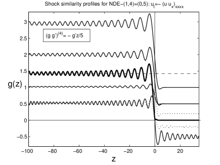
Figure 5. Various shock similarity profiles $g(z)$ as solutions of the problem (2.6), (2.9).

NDE–$(5,0)$. Consider next the first ODE (2.2) for the fully non-divergent NDE–$(5,0)$ (1.1). We can again describe formation of shocks (2.32); see Figure 6. The boldface profile with $C_{-}=1.4$ and $C_{+}=0$ has finite right-hand interface at $z=z_{0}\approx 5$, with a different expansion

(2.34) $$g(z)=\frac{6z_{0}}{5}\,(z_{0}-z)^{4}|\ln(z_{0}-z)|(1+o(1))\to 0^{+}\,\,\,\mbox{as}\,\,\,z\to z_{0}^{-}.$$

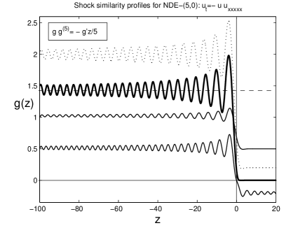
Figure 6. Various shock similarity profiles $g(z)$ as solutions of the problem (2.2), (2.9).

2.6. Shock formation for a uniformly dispersive NDE: an example

Here, as a key example to be continued, we show shocks for uniform (non-degenerate) NDEs, such as the fully divergent one,

(2.35) $$u_{t}=-((1+u^{2})u_{x})_{xxxx},$$

where the dispersion coefficient $-(1+u^{2})$ of the principal operator is an even function. Recall that, for all the previous ones (1.1)–(1.5), the dispersion coefficient is equal to $-u$ and is an odd function of $u$. Equation (2.35) is non-degenerate and represents a “uniformly dispersive” NDE. The ODE for self-similar solutions (2.1) then takes the form

(2.36) $$((1+g^{2})g^{\prime})^{(4)}=-\frac{1}{5}\,g^{\prime}z\,.$$

The mathematics of such equations is similar to that in Section 2.4. In Figure 7, we present a few shock similarity profiles for (2.36). Note that both shocks $S_{\pm}(x)$ are admissible, since for the ODE (2.36) (and for the NDE (2.35)), we have, instead of symmetry (2.8),

(2.37) $$-g(z)\quad\mbox{is also a solution}.$$

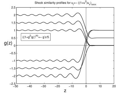
Figure 7. Various shock similarity profiles $g(z)$ satisfying the ODE (2.36).

3. (II) Riemann Problem $S_{+}$: similarity rarefaction waves

Using the reflection symmetry of all the NDEs (1.1)–(1.5),

(3.1) $$\left\{\begin{matrix}u\mapsto-u,\vskip 3.0pt plus 1.0pt minus 1.0pt\\ t\mapsto-t,\,\,\end{matrix}\right.$$

we conclude that these admit global similarity solutions defined for all $t>0$,

(3.2) $$u_{+}(x,t)=g(z),\,\,\,\mbox{with}\,\,z=x/t^{\frac{1}{5}}.$$

Then $g(z)$ solves the ODEs (2.2)–(2.6) with the opposite terms

(3.3) $$...=\frac{1}{5}\,g^{\prime}z$$

on the right-hand side. The conditions (2.7) also take the opposite form

(3.4) $$f(\pm\infty)=\pm 1.$$

Thus, these profiles are obtained from the blow-up ones in (2.1) by reflection, i.e.,

(3.5) if $$g(z) g(-z)$$ is a shock profile in (2.1), then is a rarefaction one in (3.2).

These are sufficiently regular similarity solutions of NDEs that have the necessary initial data: by Proposition 2.2(ii), in $L^{1}_{\rm loc}$,

(3.6) $$u_{+}(x,t)\to S_{+}(x)\quad\mbox{as}\quad t\to 0^{+}.$$

Other profiles $g(-z)$ from shock wave similarity patterns generate further rarefaction solutions including those with finite left-hand interfaces.

4. (III) Riemann Problem $S_{-}$: towards $\delta$-entropy test

4.1. Uniform NDEs

In this section, for definiteness, we consider the fully non-divergent NDE (1.1),

(4.1) $$u_{t}={\bf A}(u)\equiv-uu_{xxxxx}\quad\mbox{in}\quad\mathbb{R}\times(0,T),\quad u(x,0)=u_{0}(x)\in C_{0}^{\infty}(\mathbb{R}).$$

In order to concentrate on shocks and to avoid difficulties with finite interfaces or transversal zeros at which $u=0$ (these are weak discontinuities via non-uniformity of the PDE), we deal with strictly positive solutions satisfying

(4.2) $$\frac{1}{C}\leq u\leq C,\quad\mbox{where \,\, $C>1$ \,\, is a constant.}$$

Remark: uniformly non-degenerate NDEs. Alternatively, in order to avoid the assumptions like (4.2), we can consider the uniform equations such as (cf. (2.35))

(4.3) $$u_{t}=-(1+u^{2})u_{xxxxx},$$

for which no finite interfaces are available. Of course, (4.3) admits analogous blow-up similarity formation of shocks by (2.1). In Figure 8, we show a few profiles satisfying

(4.4) $$(1+g^{2})g^{(5)}=-\frac{1}{5}\,g^{\prime}z,\quad z\in\mathbb{R}.$$

Recall that, for (4.4), (2.37) holds, so both $S_{\pm}(x)$ are admissible and entropy (see below).

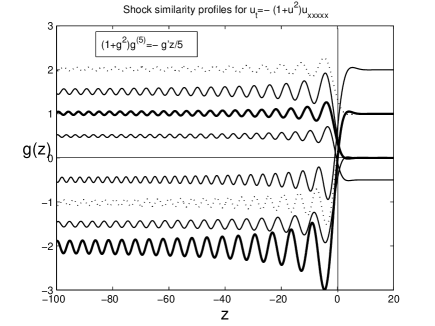
Figure 8. Various shock similarity profiles $g(z)$ satisfying the ODE (4.4).

4.2. On uniqueness, continuous dependence, and a priori bounds for smooth solutions

Actually, in our $\delta$-entropy construction, we will need just a local semigroup of smooth solutions that is continuous is $L^{1}_{\rm loc}$. The fact that such results are true for fifth-order (or other odd-order NDEs) is easy to illustrated as follows. One can see that, since (4.1) is a dispersive equation, which contains no dissipative terms, the uniqueness follows as for parabolic equations such as

$$u_{t}=-uu_{xxxx}\quad\mbox{or}\quad u_{t}=uu_{xxxxxx}\quad\big{(}\mbox{in the class}\,\,\,\big{\{}\frac{1}{C}\leq u\leq C\big{\}}\big{)}.$$

Thus, we assume that $u(x,t)$ solves (4.1) with initial data $u_{0}(x)\in H^{10}(\mathbb{R})$, satisfies (4.2), and is sufficiently smooth, $u\in L^{\infty}([0,T],H^{10}(\mathbb{R}))$, $u_{t}\in L^{\infty}([0,T],H^{5}(\mathbb{R}))$, etc. Assuming that $v(x,t)$ is the second smooth solution, we subtract equations to obtain for the difference $w=u-v$ the PDE

(4.5) $$w_{t}=-uw_{xxxxx}-v_{xxxxx}w.$$

We next divide by $u\geq\frac{1}{C}>0$ and multiply by $w$ in $L^{2}$, so integrating by parts that vanishes the dispersive term $w_{xxxxx}$ yields

(4.6) $$\int\frac{ww_{t}}{u}\equiv\frac{1}{2}\,\frac{\mathrm{d}}{{\mathrm{d}}t}\int\frac{w^{2}}{u}+\frac{1}{2}\,\int\frac{u_{t}}{u^{2}}\,w^{2}=-\int\frac{v_{xxxxx}}{u}\,w^{2}.$$

Therefore, using (4.2) and the assumed regularity yields

(4.7) $$\frac{1}{2}\,\frac{\mathrm{d}}{{\mathrm{d}}t}\int\frac{w^{2}}{u}=\int\big{(}-\frac{1}{2}\,\frac{u_{t}}{u^{2}}-\frac{v_{xxxxx}}{u}\big{)}\,w^{2}\leq C_{1}\int\frac{w^{2}}{u},$$

where the derivatives $u_{t}(\cdot,t)$ and $v_{xxxxx}(\cdot,t)$ are from $L^{\infty}([0,T])$. By Gronwall’s inequality, (4.7) yields $w(t)\equiv 0$. Obviously, these estimates can be translated to the continuous dependence result in $L^{2}$ and hence in $L^{1}_{\rm loc}$.

Other a priori bounds on solutions can be also derived along the lines of computations in [8, §§ 2, 3] that lead to rather technical manipulations. The principal fact is the same as seen from (4.7): differentiating $\alpha$ times in $x$ equation (4.1) and setting $v=D_{x}^{\alpha}u$ yields the equations with the same principal part as in (4.5):

(4.8) $$v_{t}=-uv_{xxxxx}+...\,.$$

Multiplying this by $\zeta\frac{v}{u}$, with $\zeta$ being a cut-off function, and using various interpolation inequalities makes it possible to derive necessary a priori bounds and hence to observe the corresponding smoothing phenomenon for exponentially decaying initial data.

4.3. On local semigroup of smooth solutions of uniform NDEs and linear operator theory

We recall that local $C^{\infty}$-smoothing phenomena are known for third-order linear and fully nonlinear dispersive PDEs; see [7, 8, 27, 33] and earlier references therein. We claim that, having obtained a priori bounds, a smooth local solution can be constructed by the iteration techniques as in [8, § 3] by using a standard scheme of iteration of the equivalent integral equation for spatial derivatives. We present further comments concerning other approaches to local existence, where we return to integral equations.

We then need a detailed spectral theory of fifth-order operators such as

(4.9) $$\textstyle{{\bf P}_{5}=a(x)D_{x}^{5}+b(x)D_{x}^{4}+...\,,\quad x\in(-L,L)\quad\big{(}a(x)\geq\frac{1}{C}>0\big{)},}$$

with bounded coefficients. This theory can be found in, e.g., Naimark’s book [35, Ch. 2]. For regular boundary conditions (e.g., for periodic ones that are regular for any order, which suits us well), operators (4.9) admit a discrete spectrum $\{\lambda_{k}\}$, where the eigenvalues $\lambda_{k}$ are all simple for all large $k$.

It is crucial for further use of eigenfunction expansion techniques that the complete in $L^{2}$ subset of eigenfunctions $\{\psi_{k}\}$ creates a Riesz basis, i.e., for any $f\in L^{2}$,

(4.10) $$\sum|\langle f,\psi_{k}\rangle|^{2}<\infty,\quad\mbox{where}\quad\langle f,\psi_{k}\rangle=\int f\,\overline{\psi}_{k},$$

and, for any $\{c_{k}\}\in l^{2}$ $\big{(}$i.e., $\sum|c_{k}|^{2}<\infty\big{)}$, there exists a function $f\in L^{2}$ such that

(4.11) $$\langle f,\psi_{k}\rangle=c_{k}.$$

Then there exists a unique set of “adjoint” generalized eigenfunctions $\{\psi_{k}^{*}\}$ (attributed to the“adjoint” operator ${\bf P}_{5}^{*}$) being also a Riesz basis that is bi-orthonormal to $\{\psi_{k}\}$:

(4.12) $$\langle\psi_{k},\psi_{l}^{*}\rangle=\delta_{kl}\quad\mbox{(Kronecker's delta)}.$$

Hence, for any $f\in L^{2}$, in the sense of the mean convergence,

(4.13) $$f=\sum c_{k}\psi_{k},\quad\mbox{with}\quad c_{k}=\langle f,\psi_{k}^{*}\rangle.$$

See further details in [35, § 5].

The eigenvalues of (4.9) have the asymptotics

(4.14) $$\lambda_{k}\sim(\pm 2\pi k{\rm i})^{5}\quad\mbox{for all \,\, $k\gg 1$}.$$

In particular, it is known that ${\bf P}_{5}$ has compact resolvent, which makes it possible to use it in the integral representation of the NDEs; cf. [8, § 3], where integral equations are used to construct a unique smooth solution of third-order NDEs.

On the other hand, this means that ${\bf P}_{5}-aI$ for any $a\gg 1$ is not a sectorial operator, which makes suspicious using advanced theory of analytic semigroups [9, 15, 34], as is natural for even-order parabolic flows; see further discussion below. Analytic smoothing effects for higher-order dispersive equations were studied in [51]. Concerning unique continuation and continuous dependence properties for dispersive equations, see [12] and references therein, and also [52] for various estimates.

4.4. Hermitian spectral theory and analytic semigroups

Let us continue to discuss related spectral issues for odd-order operators. For the linear dispersion equation with constant coefficients (2.13), the Cauchy problem with integrable data $u_{0}(x)$ admits the unique solution

(4.15) $$u(x,t)=b(x-\cdot,t)*u_{0}(\cdot),$$

where $b(x,t)$ is the fundamental solution (2.14). Analyticity of solutions in $t$ (and $x$) can be associated with the rescaled operator

(4.16) $$\mbox{${\bf B}_{5}=-D_{z}^{5}+\frac{1}{5}\,zD_{z}+\frac{1}{5}\,I\quad\mbox{in}\quad L^{2}_{\rho}(\mathbb{R}),$}\quad\mbox{where}\,\,\,\rho(z)=\left\{\begin{matrix}{\mathrm{e}}^{a|z|^{5/4}},\,\,\,z<0,\\ {\mathrm{e}}^{-az^{5/4}},\,\,z>0,\end{matrix}\right.$$

and $a>0$ is a sufficiently small constant. Here, ${\bf B}_{5}$ in (4.16) is the operator in (2.15) that generates the rescaled kernel $F$ of the fundamental solution in (2.14).

Next, using in (2.13) the same rescaling as in (2.14), we set

(4.17) $$u(x,t)=t^{-\frac{1}{5}}v(y,\tau),\quad y=x/t^{\frac{1}{5}},\quad\tau=\ln t,$$

to get the rescaled PDE with the operator (4.16),

(4.18) $$v_{\tau}={\bf B}_{5}v.$$

Next, on Taylor expansion of the kernel in (4.15) yields

(4.19) $$v(y,\tau)=\int F(y-z{\mathrm{e}}^{-\tau/5})\,u_{0}(z)\,{\mathrm{d}}z=\sum\limits_{(k)}\frac{(-1)^{k}}{\sqrt{k!}}\,F^{(k)}(y){\mathrm{e}}^{-\frac{k}{5}\,\tau}\frac{1}{\sqrt{k!}}\,\int z^{k}u_{0}(z)\,{\mathrm{d}}z,$$

where the series converges uniformly on compact subsets, defining an analytic solution, and also in the mean in $L^{2}_{\rho}$. According to the eigenfunctions expansion (4.19) of the semigroup, there is a proper definition of the operator (4.16) with a real spectrum and eigenfunctions (see details in [17, § 9], [20, § 8.2])

$$\sigma({\bf B}_{5})=\big{\{}-\frac{k}{5},\,k=0,1,2,...\big{\}}\quad\mbox{and}\quad\psi_{k}(y)=\frac{(-1)^{k}}{\sqrt{k!}}\,F^{(k)}(y),\,\,\,k\geq 0.$$

The basis of the “adjoint” operator (cf. (2.12)), in a space with an indefinite metric,

$${\bf B}_{5}^{*}=-D^{5}_{y}-\frac{1}{5}\,yD_{y}\quad\mbox{in}\quad L^{2}_{\rho^{*}}(\mathbb{R}),\quad\rho^{*}(z)={\mathrm{e}}^{-a|z|^{5/4}}\,\,\mbox{in}\,\,\mathbb{R},$$

has the same point spectrum and eigenfunctions $\{\psi_{k}^{*}\}$, which are generalized Hermite polynomials. Cf. a full “parabolic” version of such a Hermitian spectral theory in [13, 17]. This implies that ${\bf B}_{5}-aI$ is sectorial for $a\geq 0$ ($\lambda_{0}=0$ is simple), and this justifies the fact that (4.15) is an analytic (in $t$) flow. Let us mention again that analytic smoothing effects are well known for higher-order dispersive equations with operators of principal type, [51].

Actually, this also suggests to treat (4.1), (4.2) by a classic approach as in Da Prato–Grisvard [9] by linearizing about a sufficiently smooth $u_{0}=u(t_{0})$, $t_{0}\geq 0$, by setting $u(t)=u_{0}+v(t)$ giving the linearized equation

(4.20) $$v_{t}={\bf A}^{\prime}(u_{0})v+{\bf A}(u_{0})+g(v),\quad t>t_{0};\quad v(t_{0})=0,$$

where $g(v)$ is a quadratic perturbation. Using the good semigroup ${\mathrm{e}}^{{\bf A}^{\prime}(u_{0})t}$, this makes it possible to study local regularity properties of the corresponding integral equation

(4.21) $$v(t)=\int\limits_{t_{0}}^{t}{\mathrm{e}}^{{\bf A}^{\prime}(u_{0})(t-s)}({\bf A}(u_{0})+g(v(s)))\,{\mathrm{d}}s.$$

Note that this smoothing approach demands a fast exponential decay of solutions $v(x,t)$ as $x\to\infty$, since one needs that $v(\cdot,t)\in L^{2}_{\rho}$; cf. [33], where $C^{\infty}$-smoothing for third-order NDEs was also established under the exponential decay. Equation (4.21) can be used to guarantee local existence of smooth solutions of a wide class of odd-order NDEs.

Thus, we state the following conclusion to be used later on:

(4.22) $$\begin{matrix}\mbox{any sufficiently smooth solution $u(x,t)$ of (\ref{ss1}), (\ref{ss2}) at $t=t_{0}$,}\vskip 3.0pt plus 1.0pt minus 1.0pt\\ \mbox{can be uniquely extended to some interval $t\in(t_{0},t_{0}+\nu)$, $\nu>0$.}\end{matrix}$$

4.5. Smooth deformations and $\delta$-entropy test for solutions with shocks

The situation dramatically changes if we want to treat solutions with shocks. Namely, it is known that even for the NDE–3 (1.30), the similarity formation mechanism of shocks immediately shows nonunique extensions of solutions after a typical “gradient” catastrophe [21]. Therefore, we do not have a chance to get, in such an easy (or any) manner, a uniqueness/entropy result for more complicated NDEs such as (1.5) by using the $\delta$-deformation (evolutionary smoothing) approach. However, we will continue using these ideas, turned out to be fruitful, in order to develop a much weaker “$\delta$-entropy test” for distinguishing some simple shock and rarefaction waves.

Thus, given a small $\delta>0$ and a sufficiently small bounded continuous (and, possibly, compactly supported) solution $u(x,t)$ of the Cauchy problem (4.1), satisfying (4.2), we construct its smooth $\delta$-deformation, aiming get smoothing in a small neighbourhood of bounded shocks, as follows. Note that we deal here with simple shock configurations (mainly, with 1-shock structures), and do not aim to cover more general shock geometry, which can be very complicated; especially since we do not know all types of simple single-point moving shocks.

(i) We perform a smooth $\delta$-deformation of initial data $u_{0}(x)$ by introducing a suitable $C^{1}$ function $u_{0\delta}(x)$ such that

(4.23) $$\int|u_{0}-u_{0\delta}|<\delta.$$

If $u_{0}$ is already sufficiently smooth, this step must be abandoned (now and always later on). By $u_{1\delta}(x,t)$, we denote the unique local smooth solution of the Cauchy problem with data $u_{0\delta}$, so that, by (4.22), the continuous function $u_{1\delta}(x,t)$ is defined on the maximal interval $t\in[t_{0},t_{1}(\delta))$, where we denote $t_{0}=0$ and $t_{1}(\delta)=\Delta_{1\delta}$. At this step, we are able to eliminate non-evolution (evolutionary unstable) initially posed shocks, which then create corresponding smooth rarefaction waves.

(ii) At $t=\Delta_{1\delta}$, a shock-type discontinuity (or possibly infinitely many shocks) is supposed to occur, since otherwise we extend the continuous solution by (4.22), so we perform another suitable $\delta$-deformation of the “data” $u_{1\delta}(x,\Delta_{1\delta})$ to get a unique continuous solution $u_{2\delta}(x,t)$ on the maximal interval $t\in[t_{1}(\delta),t_{2}(\delta))$, with $t_{2}(\delta)=\Delta_{1\delta}+\Delta_{2\delta}$, etc. Here and in what follows, we always mean a “$\delta$-smoothing” performed in a small neighbourhood of occurring singularities only as discontinuous shocks.

$\dots$

We continue in this manner with suitable choices of each $\delta$-deformations of “data” at the moments $t=t_{j}(\delta)$, when $u_{j\delta}(x,t)$ has a shock, there exists a $t_{k}(\delta)>1$ for some finite $k=k(\delta)$, where $k(\delta)\to+\infty$ as $\delta\to 0$. It is easy to see that, for bounded solutions, $k(\delta)$ is always finite. A contradiction is obtained by assuming that $t_{j}(\delta)\to\bar{t}<1$ as $j\to\infty$ for arbitrarily small $\delta>0$ meaning a kind of “complete blow-up” that was excluded by assumption of smallness of the data.

This gives a global $\delta$-deformation in $\mathbb{R}\times[0,1]$ of the solution $u(x,t)$, which is the discontinuous orbit denoted by

(4.24) $$u^{\delta}(x,t)=\{u_{j\delta}(x,t)\,\,\,\mbox{for}\,\,\,t\in[t_{j-1}(\delta),t_{j}(\delta)),\quad j=1,2,...,k(\delta)\}.$$

One can see that this $\delta$-deformation construction aims at checking a kind of evolution stability of possible shock wave singularities and therefore, to exclude those that are not entropy and evolutionarily generate smooth rarefaction waves.

Finally, by an arbitrary smooth $\delta$-deformation, we will mean the function (4.24) constructed by any sufficiently refined finite partition $\{t_{j}(\delta)\}$ of $[0,1]$, without reaching a shock of $S_{-}$-type at some or all intermediate points $t=t_{j}^{-}(\delta)$.

We next say that, given a solution $u(x,t)$, it is stable relative smooth deformations, or simply $\delta$-stable ($\delta$eformation-stable), if for any $\varepsilon>0$, there exists $\delta=\delta(\varepsilon)>0$ such that, for any finite $\delta$-deformation of $u$ given by (4.24),

(4.25) $$\iint|u-u^{\delta}|<\varepsilon.$$

Recall that (4.24) is an $\delta$-orbit, and, in general, is not and cannot be aimed to represent a fixed solution in the limit $\delta\to 0$; see below.

4.6. On $\delta$-entropy solutions

Having checked that the local smooth solvability problem above is well-posed, we now present the corresponding definition that will be applied to particular weak solutions. Recall that the metric of convergence, $L^{1}_{\rm loc}$ under present consideration, for (1.30) was justified by a similarity analysis presented in Proposition 2.2. For other types of shocks and/or NDEs, the metric may be different.

Thus, under the given hypotheses, a function $u(x,t)$ is called a $\delta$-entropy solution of the Cauchy problem $(\ref{ss1})$, if there exists a sequence of its smooth $\delta$-deformations $\{u^{\delta_{k}},\,k=1,2,...\}$, where $\delta_{k}\to 0$, which converges in $L^{1}_{\rm loc}$ to $u$ as $k\to\infty$.

This is slightly weaker (but equivalent) to the condition of $\delta$-stability.

Remark: $\delta$-entropy solution is unique for 1D conservation law. Consider, as a typical example, (1.7) for general measurable $L^{1}$-data. The classical Oleinik–Kruzhkov’s entropy theory for (1.7) defines the unique semigroup of contractions in $L^{1}$ (see [50]), i.e., for an arbitrary pair of entropy solutions $u(\cdot,t)$ and $v(\cdot,t)$, in the sense of distributions,

(4.26) $$\frac{{\mathrm{d}}}{{\mathrm{d}}t}\,\|u(t)-v(t)\|_{L^{1}}\leq 0\quad\mbox{for a.a. $t\geq 0$}.$$

Consider now the above $\delta$-deformation construction of an orbit $\{u_{\delta}\}$ in the case, when the entropy solution $u(x,t)$ is continuous a.e. for all $t\geq 0$, i.e., shocks have zero measure. It means that $u_{\delta}(x,t)$ for $t\geq 0$ is smooth and essentially differs from $u(x,t)$ on a set of arbitrarily small measure $\sim\delta\to 0$. Therefore, under these (possibly, non-constructive) assumptions, (4.26) implies that any smooth $\delta$-deformations in $L^{1}$ inevitably lead to the unique entropy solution of (1.7) as $\delta\to 0$. In other words,

(4.27) for Euler’s equation (1.7), classic entropy solutions $$= \delta$$ -entropy ones.

Of course, this is just the trivial consequence of the $L^{1}$-contractivity (4.26), which, in its turn, is induced by the Maximum Principle. It is also worth mentioning that, somehow, (4.26) reflects the fact that the conservation laws such as (1.7) admit the direct algebraic solution via characteristics. Indeed, the characteristic method guarantees the unique solvability in the regularity domain, while the “shocks cut off” can be performed at necessary points by the corresponding Rankine–Hugoniot relations. Thus, the entropy conditions just describe the correct evolution from initially posed singularities (evolutionary, such “rarefaction waves” cannot appear by characteristics).

Therefore, the absence of the Maximum Principle and absence of any characteristic-based approaches for higher-order NDEs recall that a result such as (4.27) cannot be expected in principle here. The situation is even more terrible: we will show that any uniqueness/entropy results for such NDEs fail always and anyway.

4.7. $\delta$-entropy test and nonexistent uniqueness

Since, for obvious reasons, the $\delta$-deformation construction gets rid of non-evolutionary shocks (leading to non-singular rarefaction waves), a first consequence of the construction is that it defines the $\delta$-entropy test for solutions, which allows one, at least, to distinguish the true simple isolated shocks from smooth rarefaction waves.

In Section 5, we show that it is completely unrealistic to expect from this construction something essentially stronger in the direction of uniqueness and/or entropy-like selection of proper solutions. Though these expectations correspond well to previous classical PDE entropy-like theories, these are excessive for higher-order models, where such a universal property is not achievable at all any more. Even proving convergence for a fixed special $\delta$-deformation is not easy at all. Thus, for particular cases, we will use the above notions with convergence along a subsequence of $\delta$’s to classify and distinguish shocks and rarefaction waves of simple geometric configurations:

4.8. First easy conclusions of $\delta$-entropy test

As a first application, we have:

Proposition 4.1.

Shocks of the type $S_{-}(x)$ are $\delta$-entropy for $(\ref{ss1})$.

The result follows from the properties of similarity solutions (2.1), with $-t\mapsto T_{t}$, which, by varying the blow-up time $T\mapsto T+\delta$, can be used as their local smooth $\delta$-deformations at any point $t\geq 0$.

Proposition 4.2.

Shocks of the type $S_{+}(x)$ are not $\delta$-entropy for $(\ref{ss1})$.

Indeed, taking initial data $S_{+}(x)$ and constructing its smooth $\delta$-deformation via the self-similar solution (3.2) with shifting $t\mapsto t+\delta$, we obtain the global $\delta$-deformation $\{u^{\delta}=u_{+}(x,t+\delta)\}$, which goes away from $S_{+}$.

Thus, the idea of smooth $\delta$-deformations allows us to distinguish basic $\delta$-entropy and non-entropy shocks without any use of mathematical manipulations associated with standard entropy inequalities, which, indeed, are illusive for higher-order NDEs; cf. [21]. We believe that successful applications of the $\delta$-entropy test can be extended to any configuration with a finite number of isolated shocks. However, it is completely illusive to think that such a simple procedure could be applied to general solutions, especially since the uniqueness after singularity formation cannot be achieved in principle, as we show next.

In other words, the $\delta$-entropy test allows us to prohibit formation of non $\delta$-deformation stable shocks of type $S_{+}$ and proposes a smooth rarefaction wave instead. However, this approach cannot detect a unique shock of the opposite geometry $S_{-}$, since such a formation is principally nonunique.

5. (IV) Nonuniqueness after shock formation

Here we mainly follow the ideas from [21] applied there to the NDE–3 (1.30), so we will omit some technical data and present more convincing analytic and numerical results concerning the nonuniqueness. For the hard 5D dynamical systems under consideration, numerics becomes more and more essential and unavoidable for understanding the nature of such nonunique extensions of solutions. Without loss of generality, we always deal with the NDE–5 (1.5) of the fully divergent form.

5.1. Main strategy towards nonunique continuation: pessimistic conclusions

We begin with the study of new shock patterns, which are induced by other (cf. (2.1)) similarity solutions of (1.5):

(5.1) $$u_{-}(x,t)=(-t)^{\alpha}f(y),\quad y=\frac{x}{(-t)^{\beta}},\quad\beta=\frac{1+\alpha}{5},\quad\mbox{where $\alpha\in\big{(}0,\frac{1}{4}\big{)}$ and}$$

(5.2) $$\left\{\begin{matrix}-(ff^{\prime})^{(4)}-\beta f^{\prime}y+\alpha f=0\quad\mbox{in}\quad\mathbb{R}_{-},\quad f(0)=f^{\prime\prime}(0)=f^{(4)}(0)=0,\vskip 3.0pt plus 1.0pt minus 1.0pt\\ f(y)=C_{0}|y|^{\frac{\alpha}{\beta}}(1+o(1))\quad\mbox{as}\quad y\to-\infty,\quad C_{0}>0.\qquad\qquad\qquad\quad\,\,\,\end{matrix}\right.$$

In this section, in order to match the key results in [21], in (2.1) and later on, we change the variables $\{g,z\}\mapsto\{f,y\}$. In the next Section 6, we return to the original notation. The anti-symmetry conditions in (5.2) allow us to extend the solution to the positive semi-axis $\{y>0\}$ by the reflection $-f(-y)$ to get a global pattern.

Obviously, the solutions (2.1), which are suitable for Riemann problems, correspond to the simple case $\alpha=0$ in (5.1). It is easy to see that, for positive $\alpha$, the asymptotics in (5.2) ensures getting first gradient blow-up at $x=0$ as $t\to 0^{-}$, as a weak discontinuity, where the final time profile remains locally bounded and continuous:

(5.3) $$u_{-}(x,0^{-})=\left\{\begin{matrix}C_{0}|x|^{\frac{\alpha}{\beta}}\,\,\,\,\quad\mbox{for}\quad x<0,\vskip 3.0pt plus 1.0pt minus 1.0pt\\ -C_{0}|x|^{\frac{\alpha}{\beta}}\quad\mbox{for}\quad x>0,\end{matrix}\right.$$

where $C_{0}>0$ is an arbitrary constant. Note that the standard “gradient catastrophe”, $u_{x}(0,0^{-})=-\infty$, then occurs in the range, which we will deal within,

(5.4) $$\frac{\alpha}{\beta}<1\quad\mbox{provided that}\quad\alpha<\frac{1}{4}.$$

Thus, the wave braking (or “overturning”) begins at $t=0$, and next we show that it is performed again in a self-similar manner and is described by similarity solutions

(5.5) $$u_{+}(x,t)=t^{\alpha}F(y),\quad y=\frac{x}{t^{\beta}},\quad\beta=\frac{1+\alpha}{5},\quad\mbox{where}$$

(5.6) $$\left\{\begin{matrix}-(FF^{\prime})^{(4)}+\beta F^{\prime}y-\alpha F=0\quad\mbox{in}\quad\mathbb{R}_{-},\qquad\qquad\qquad\qquad\quad\,\,\vskip 3.0pt plus 1.0pt minus 1.0pt\\ F(0)=F_{0}>0,\,\,\,F(y)=C_{0}|y|^{\frac{\alpha}{\beta}}(1+o(1))\quad\mbox{as}\quad y\to-\infty,\end{matrix}\right.$$

where the constant $C_{0}>0$ is fixed by blow-up data (5.3). The asymptotic behaviour as $y\to-\infty$ in (5.6) guarantees the continuity of the global discontinuous pattern (with $F(-y)\equiv-F(y)$) at the singularity blow-up instant $t=0$, so that

(5.7) $$u_{-}(x,0^{-})=u_{+}(x,0^{+})\quad\mbox{in}\quad\mathbb{R}.$$

Then any suitable couple $\{f,F\}$ defines a global solution $u_{\pm}(x,t)$, which is continuous at $t=0$, and then it is called an extension pair. It was shown in [21] that, for the typical NDEs–3, the pair is not uniquely determined and there exist infinitely many shock-type extensions of the solution after blow-up at $t=0$. We are going to describe a similar nonuniqueness phenomenon for the NDEs–5 such as (1.5).

It is worth mentioning that, for conservation laws such as (1.7), such an extension pair $\{f,F\}$ is always unique; see similarity analysis in [21, § 4]. Of course, this is not surprising due to existing Oleinik–Kruzhkov’s classic uniqueness-entropy theory [37, 31]. Note again that any sufficient multiplicity of extension pairs $\{f,F\}$, obtained via small micro-scale blow-up analysis of the PDEs, would always lead to a principle nonuniqueness, so this approach could be referred to as a “uniqueness test”.

A first immediate consequence of our similarity blow-up/extension analysis is as follows:

(5.8) in the CP, formation of shocks for the NDE (1.5) can lead to nonuniqueness.

The second conclusion is more subtle and is based on the fact that, for some initial data at $t=0$ (i.e., created by single point gradient blow-up as $t\to 0^{-}$), the whole admitted solution set for $t>0$ does not contain any “minimal”, “maximal”, “extremal” in any reasonable sense, or any isolated points, which might play a role of a unique “entropy” one chosen by introducing a hypothetical entropy inequalities, conditions, or otherwise. If this is true for the whole set of such weak solutions of (1.5) with initial data (5.3), then, for the Cauchy problem,

(5.9) there exists no general “entropy mechanisms” to choose a unique solution.

Actually, overall, (5.8) and (5.9) show that the problem of uniqueness of weak solutions for the NDEs such as (1.5) cannot be solved in principal.

On the other hand, in a FBP setting by adding an extra suitable condition on shock lines, the problem might be well-posed with a unique solution, though proofs can be very difficult. We refer again to a more detailed discussion of these issues for the NDE–3 (1.30) in [21]. Though we must admit that, for the NDE–5 (1.5), which induces 5D dynamical systems for the similarity profiles (and hence 5D phase spaces), those nonuniqueness and non-entropy conclusions are more difficult and not that clear as for the NDEs–3, so some of their aspects do unavoidably remain questionable and even open.

Hence, the nonuniqueness in the CP is a non-removable issue of PDE theory for higher-order degenerate nonlinear odd-order equations (and possibly not only for those). The nonuniqueness of solutions of (1.5) has some pure dimensional natural features, and, more precisely, is associated with the dimensions of “good” and “bad” asymptotic bundles of orbits in the 5D phase space of the ODE (5.6).

5.2. Infinite shock similarity solutions for $\alpha<0$

Let us first note that the blow-up solutions (5.1) represent an effective way to describe other types of singularities with infinite shocks. Namely, assuming that

(5.10) $$\alpha<0\quad\mbox{and}\quad\frac{\alpha}{\beta}<0,$$

we again obtain the same “data” (5.3) but now $u_{-}(0,0^{-})=\infty$. We do not study in any detail such interesting new singularity phenomena and present Figure 9 showing that such infinite shock similarity profiles do exist. For comparison, we indicate the standard $S_{-}$-type profile for $\alpha=0$, which coincides with that in Figure 3(d).

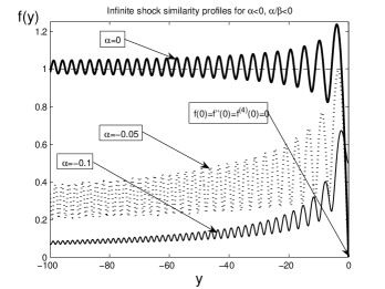
Figure 9. Infinite shock similarity profiles as solutions of (5.2) for $\alpha<0$: $\alpha=-0.05$ and $\alpha=-0.1$.

For the NDE–3 such as (1.30), the infinite shock similarity solutions in the range (5.10) were studied in [23, § 4] in sufficient detail.

5.3. Gradient blow-up similarity solutions

Consider the blow-up ODE problem (5.2), which is a difficult one, with a 5D phase space. Note that, by invariant scaling (2.22), it can be reduced to a 4th-order ODE with a also even more complicated nonlinear operator composed from too many polynomial terms, so we do not rely on that and work in the original phase space. Therefore, some more delicate issues on, say, uniqueness of certain orbits, become very difficult or even remain open, though some more robust properties can be detected rigorously. We will also use numerical methods for illustrating and even justifying some of our conclusions. As before, for the fifth-order equations such as (5.2), this and further numerical constructions are performed by the MatLab with the standard ode45 solver therein.

Let us describe the necessary properties of orbits $\{f(y)$} we are interested in. Firstly, it follows from the conditions in (5.2) that, for $y\approx 0^{-}$,

(5.11) the set of proper orbits is 2D parameterized by $$f_{1}=f^{\prime}(0)<0 f_{3}=f^{\prime\prime\prime}(0)$$ and .

Secondly and on the other hand, the necessary behaviour at infinity is as follows:

(5.12) $$f(y)=C_{0}|y|^{\frac{5\alpha}{1+\alpha}}(1+o(1))\quad\mbox{as}\quad y\to-\infty\quad\big{(}\frac{5\alpha}{1+\alpha}=\frac{\alpha}{\beta}\big{)},$$

where $C_{0}>0$ is an arbitrary constant by scaling (2.22). It is key to derive the whole 4D bundle of solutions satisfying (5.12). This is done by the linearization as $y\to-\infty$:

(5.13) $$\begin{split}&f(y)=f_{0}(y)+Y(y),\quad\mbox{where}\quad f_{0}(y)=C_{0}(-y)^{\frac{\alpha}{\beta}}\vskip 3.0pt plus 1.0pt minus 1.0pt\\ \quad\Longrightarrow\quad&\mbox{$-C_{0}((-y)^{\frac{\alpha}{\beta}}Y)^{(5)}+\beta Y^{\prime}(-y)+\alpha Y+\frac{1}{2}\,(f_{0}^{2}(y))^{(5)}+...=0.$}\end{split}$$

By WKBJ-type asymptotic techniques in ODE theory, solutions of (5.13) have a standard exponential form with the characteristic equation:

(5.14) $$Y(y)\sim{\mathrm{e}}^{a(-y)^{\gamma}},\,\,\,\gamma=1+\frac{1}{4}\,\big{(}1-\frac{\alpha}{\beta}\big{)}>1\quad\Longrightarrow\quad C_{0}(\gamma a)^{4}=\beta,$$

which has three roots with non-positive real parts, ${\rm Re}\,a_{k}\leq 0$, where $a_{1}<0$ is real and conjugate $a_{2,3}\in{\rm i}\,\mathbb{R}$. Hence, we conclude that:

(5.15) as $$y\to-\infty C_{0}$$, the bundle (5.12) is four-dimensional (including ).

The behaviour corresponding the bundle (5.15) gives the desired asymptotics. Indeed, by (5.12), we have the gradient blow-up behaviour at a single point: for any fixed $x<0$, as $t\to 0^{-}$, where $y=x/(-t)^{\beta}\to-\infty$, uniformly on compact subsets,

(5.16) $$u_{-}(x,t)=(-t)^{\alpha}f(y)=(-t)^{\alpha}C_{0}\big{|}\frac{x}{(-t)^{\beta}}\big{|}^{\frac{\alpha}{\beta}}(1+o(1))\to C_{0}|x|^{\frac{5\alpha}{1+\alpha}}.$$

Let us explain some other crucial properties of the phase space, now meaning “bad bundles” of orbits. First, these are the fast growing solutions according to the explicit solution

(5.17) $$f_{\rm*}(y)=-\frac{y^{5}}{15120}>0\quad\mbox{for}\quad y\ll-1.$$

Analogously to (5.13), we compute the whole bundle about (5.17):

(5.18) $$f(y)=f_{*}(y)+Y(y)\quad\Longrightarrow\quad\mbox{$\frac{1}{15120}\,(y^{5}Y)^{(5)}-\beta Y^{\prime}y+\alpha Y+...=0.$}$$

This Euler equation has the following solutions with the characteristic polynomial:

(5.19) $$Y(y)=y^{m}\quad\Longrightarrow\quad h_{\alpha}(m)\equiv\frac{(m+1)(m+2)(m+3)(m+4)(m+5)}{15120}-\beta m+\alpha=0.$$

One root $m=-5$ is obvious that gives the solution (5.17). It turns our that this algebraic equation has precisely five negative real roots for $\alpha$ from the range (5.4), as Figure 10 shows. Actually, (b) explains that the graphs are rather slightly dependent on $\alpha$. Thus:

(5.20) the bundle about (5.17) is five-dimensional.

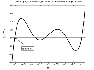
(a) $\alpha=\frac{1}{9}$

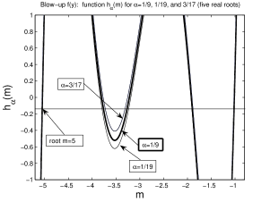
(b) various $\alpha$

Figure 10. The polynomial $h_{\alpha}(m)$ in (5.19) for various $\alpha\in\big{(}0,\frac{1}{4}\big{)}$: five negative roots.

Second, there exists a bundle of positive solutions vanishing at some finite $y\to y_{0}^{+}<0$ with the behaviour (this bundle occurs from both sides, as $y\to y_{0}^{\pm}$ to be also used)

(5.21) $$f_{1}(y)=A\sqrt{|y-y_{0}|}\,(1+o(1)),\quad A>0,$$

is 4D, which also can be shown by linearization about (5.21). Indeed, the linearized operator contains the leading term

(5.22) $$-A^{2}(\sqrt{|y-y_{0}|}\,\,Y)^{(5)}+...=0\quad\Longrightarrow\quad Y(y)\sim|y-y_{0}|^{\frac{3}{2}},\,\,\,|y-y_{0}|^{\frac{5}{2}},\,\,\,|y-y_{0}|^{\frac{7}{2}},$$

which together with the parameter $y_{0}<0$ yields

(5.23) the bundle about (5.21) is four-dimensional.

Thus, (5.11), (5.15), (5.20), and (5.23) prescribe key aspects of the 5D phase space we are dealing with. To get a global orbit $\{f(y),\,y\in\mathbb{R}_{-}\}$ as a connection of the proper bundles (5.11) and (5.15), it is natural to follow the strategy of “shooting from below” by avoiding the bundle (5.21), (5.23), i.e., using the parameters $f_{1,3}$ in (5.11), to obtain

(5.24) $$y_{0}=-\infty.$$

It is not difficult to see that this profile $f(y)$ will belong to the bundle (5.15). The proof of such a 2D shooting strategy can be done by standard arguments. By scaling (2.22), we always can reduce the problem to a 1D shooting (recall that $f_{0}=f_{2}=f_{4}=0$ already):

(5.25) $$f_{1}\equiv f^{\prime}(0)=-1\quad\mbox{and}\quad f_{3}\equiv f^{\prime\prime\prime}(0)\,\,\,\mbox{is a parameter.}$$

By the above asymptotic analysis of the 5D phase space, it follows that:

(I) for $f_{3}\ll-1$ the orbit belongs to the bundle about (5.17), and

(II) for $f_{3}\gg 1$, the orbit vanishes at finite $y_{0}$ along (5.21).

Hence, by continuous dependence, we obtain a solution $f(y)$ by the min-max principle (plus some usual technical details that can be omitted). Before stating the result, for convenience, in Figure 11, obtained by the ode45 solver, we explain how we are going to justify existence of a proper blow-up shock profile $f(y)$; cf. Figure 4.

Thus, we fix the above speculations as follows:

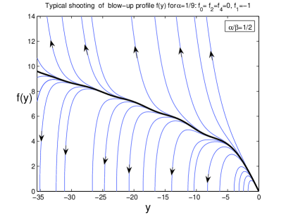
Figure 11. The shooting strategy of a blow-up similarity profile $f(y)$ for $\alpha=\frac{1}{9}$, with data $f(0)=f^{\prime\prime}(0)=f^{(4)}(0)=0$ and $f^{\prime}(0)=1$; the shooting parameter is $f^{\prime\prime\prime}(0)=0.0718040128557...$ .

Proposition 5.1.

(i) In the range $(\ref{Ran1})$, the problem $(\ref{s2a})$ admits a shock profile $f(y)$.

We have the following expectation: (ii) $f(y)$ is unique up to scaling $(\ref{2.8})$ and is positive for $y<0$. This remains an open problem that was confirmed numerically. In [21], for the NDE–3 (1.30), the phase space is 3D and a full proof is available.

In fact, this is a rather typical result for higher-order dynamical systems. E.g., we refer to a similar and not less complicated study of a 4th-order ODE [25], where existence and uniqueness of a positive solution of the radial bi-harmonic equation with source:

(5.26) $$\Delta^{2}_{r}u=u^{p}\quad\mbox{for}\quad r=|x|>0,\quad u(0)=1,\quad u^{\prime}(0)=u^{\prime\prime\prime}(0)=0,\quad u(\infty)=0,$$

was proved in the supercritical Sobolev range $p>p_{\rm Sob}=\frac{N+4}{N-4}$, $N>4$. Here, analogously, there exists a single shooting parameter being the second derivative at the origin $u_{2}=u^{\prime\prime}(0)$; the value $u_{0}=u(0)=1$ is fixed by a scaling symmetry. Proving uniqueness of such a solution in [25] is not easy and leads to essential technicalities, which the attentive reader can consult in case of necessity. Fortunately, we are not interested in any uniqueness of such kind. Instead of the global behaviour such as (5.17), the equation (5.26) admits the blow-up one governed by the principal operator $u^{(4)}+...=u^{p}\quad(u\to+\infty).$ The solutions vanishing at finite point otherwise can be treated as in the family (I).

More numerics by bvp4c. We next use more advanced and enhanced numerical methods towards existence (and uniqueness-positivity, see (ii)) of $f(y)$. Figure 12 shows blow-up profiles, with $f(0)=0$, constructed by a different method (via the solver bvp4c) for convenient values $\alpha=\frac{1}{9}$, $\frac{1}{19}$, and $\frac{3}{17}$. Note the clear oscillatory behaviour of such patterns that is induces by complex roots of the characteristic equation (5.14).

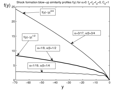
Figure 12. The odd blow-up similarity profiles $f(y)$ in $\mathbb{R}_{-}$ with $\alpha=\frac{1}{9}$, $\frac{1}{19}$, and $\frac{3}{17}$.

Collapse of shocks: “backward nonuniqueness”. This new phenomenon is presented in Figure 13, which shows the shooting from $y=0^{-}$ for

(5.27) $$\alpha=\frac{1}{9}\quad\Longrightarrow\quad\frac{\alpha}{\beta}=\frac{1}{2}.$$

This again illustrates the actual strategy in proving Proposition 5.1. However, though the phase space looks similar, note that here, as an illustration of another important evolution phenomenon, we solve the problem with $f(0)\neq 0$, so that there exists a non-zero jump of $u_{-}(x,t)$ at $x=0$ denoted by $[\cdot]$:

(5.28) $$f(0)=f_{0}=10\quad\Longrightarrow\quad[u_{-}(0,t)]=2f_{0}(-t)^{\alpha}\to 0\quad\mbox{as}\quad t\to 0^{-}.$$

Therefore, this similarity solution describes collapse of a shock wave as $t\to 0^{-}$.

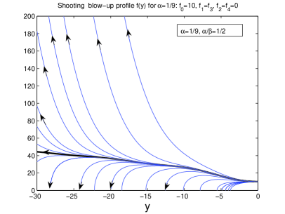
Figure 13. Shooting the blow-up profile $f(y)$ for $\alpha=\frac{1}{9}$: $f(0)=10$, $f^{\prime\prime}(0)=f^{(4)}(0)=0$ and the shooting parameter is $f^{\prime}(0)=f^{\prime\prime\prime}(0)$.

More numerical results of such types are presented in Figures 14 and 15, where we use other boundary conditions at $y=0$. Note that, being extended for $y>0$ in the anti-symmetric way, by $-f(-y)$, this will give a proper shock wave solution with the nil speed of propagation (see the R–H condition (5.42) below).

In a whole, since all these blow-up profiles satisfy the necessary behaviour as $y\to-\infty$ as indicated in (5.2), these create as $t\to 0^{-}$ the same initial data (5.3). This confirms the following phenomenon of “backward nonuniqueness”: initial data $(\ref{s3a})$ with gradient blow-up at $x=0$ can be created by an infinite number $($in fact, by a 2D subset parameterized, say, by $\{f_{0},f_{1}\})$ of various self-similar solutions $(\ref{s1a})$.

Indeed, such a nonuniqueness is directly associated with the fact that, due to (5.15), the proper asymptotic bundle as $y\to-\infty$ is 3D (for a fixed $C_{0}>0$, we have to subtract the dimension via the scaling invariance (2.22)). Therefore, roughly speaking, shooting from $y=0^{-}$ with 5 parameters $f_{0}=f(0)$, … , $f_{4}=f^{(4)}(0)$ allows a 2D ($2=5-3$) subset of solutions $f(y)$ with shocks at $y=0$. A full justification of such a conclusion requires a more careful analysis of the phase space including geometry of two “bad” bundles, which we do not perform here concentrating on other more important solutions and true nonuniqueness phenomena.

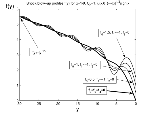
Figure 14. Blow-up profiles $f(y)$ for $\alpha=\frac{1}{9}$, with $f^{\prime}(0)=-1$, $f^{\prime\prime}(0)=0$; $f(0)\in[0,1.5]$ being a parameter.

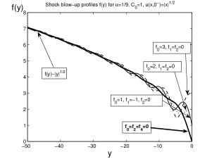
(a) $f^{\prime}(0)=f^{\prime\prime}(0)=0$

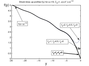
(b) $f^{\prime\prime}(0)=\frac{1}{2}$, $f^{(4)}(0)=0$

Figure 15. Blow-up profiles $f(y)$ for $\alpha=\frac{1}{9}$, for $f^{\prime}(0)=f^{\prime\prime}(0)=0$ (a) and $f^{\prime\prime}(0)=\frac{1}{2}$, $f^{(4)}(0)=0$ (b); $f(0)$ is a parameter.

Stationary solutions with a “weak shock”. The ODE in (5.2) and hence the PDE (1.5) admit a number of simple continuous “stationary” solutions. E.g., consider

(5.29) $$\alpha=\frac{1}{9},\,\,\frac{\alpha}{\beta}=\frac{1}{2}:\quad\hat{f}(y)=\sqrt{|y|}\,\,{\rm sign}\,y\quad\mbox{and}\quad\hat{u}(x,t)\equiv\pm\sqrt{|x|}\,\,{\rm sign}\,x.$$

Note that these are not weak solutions of the stationary equation

(5.30) $$\frac{1}{2}\,(u^{2})_{xxxxx}=0\quad\mbox{in}\quad{\mathcal{D}}^{\prime}.$$

The classic stationary solution of (5.30) $\hat{u}(x,t)=\pm x^{2}$ is smoother at $x=0$.

We will show that such “weak stationary shocks” as in (5.29) also lead to nonuniqueness.

Remark: an exact solution for a critical $\alpha$. One can see that the quadratic operator ${\bf B}(f)=(ff^{\prime})^{(4)}$ in (5.2) admits the following polynomial invariant subspace:

$$W_{6}={\rm Span}\{1,y,y^{2},y^{3},y^{4},y^{5}\}\quad\Longrightarrow\quad{\bf B}(W_{6})\subseteq W_{6}.$$

Restricting the ODE (5.2) to $W_{6}$ yields an algebraic system, which admits an exact solution for the following value of the critical $\alpha_{\rm c}$:

(5.31) $$\alpha=\alpha_{\rm c}=\frac{17}{84}=0.202381...\quad\Longrightarrow\quad\exists\,\,f(y)=Cy-\frac{4!}{9!}\,y^{5},\,\,\,C\in\mathbb{R}.$$

Since $\alpha_{\rm c}>0$, it does not deliver a “saw”-type blow-up profile (having infinite number of positive humps) as it used to be for the NDE–3 (1.30) for $\alpha_{\rm c}=-\frac{1}{10}$; see [23, § 4].

5.4. Nonuniqueness of similarity extensions beyond blow-up

As in [21] for the NDEs–3, a discontinuous shock wave extension of blow-up similarity solutions (5.1), (5.2) is assumed to be done by using the global ones (5.5), (5.6). Actually, this leads to watching a whole 5D family of solutions parameterized by their Cauchy values at the origin:

(5.32) $$F(0)=F_{0}>0,\,\,\,F^{\prime}(0)=F_{1}<0,\,\,\,F^{\prime\prime}(0)=F_{2},\,\,\,F^{\prime\prime\prime}(0)=F_{3},\,\,\,F^{(4)}(0)=F_{4}.$$

Thus, unlike (5.11), the proper bundle in (5.32) is 5D. Note that at $y=-\infty$, the solution must have the form

(5.33) $$F(y)=C_{0}|y|^{\frac{5\alpha}{1+\alpha}}(1+o(1))\quad\mbox{as}\quad y\to-\infty\quad(C_{0}>0).$$

As above, the 5D phase space for the ODE in (5.6) has two stable “bad” bundles:

(I) Positive solutions with “singular extinction” in finite $y$, where $F(y)\to 0$ as $y\to y_{0}^{+}<0$. This is an unavoidable singularity following from the degeneracy of the equations with the principal term $FF^{(5)}$ leading to the singular potential $\sim\frac{1}{F}$. As in (5.22), this bundle is 4D, and

(II) Negative solutions with the fast growth (cf. (5.17)):

(5.34) $$F_{*}(y)=\frac{y^{5}}{15120}\,(1+o(1))\to-\infty\quad\mbox{as}\quad y\to-\infty.$$

The characteristic polynomial is the same as in (5.19), so that the bundle is 5D; cf. (5.20).

Both sets of such solutions are open by the standard continuous dependence of solutions of ODEs on parameters. The whole bundle of solutions satisfying (5.12) is obtained by linearization as $y\to-\infty$ in (5.6):

(5.35) $$\begin{split}&f(y)=F_{0}(y)+Y(y),\quad\mbox{where}\quad F_{0}(y)=C_{0}(-y)^{\frac{\alpha}{\beta}}\vskip 3.0pt plus 1.0pt minus 1.0pt\\ \quad\Longrightarrow\quad&\mbox{$-C_{0}((-y)^{\frac{\alpha}{\beta}}Y)^{(5)}-\beta Y^{\prime}(-y)-\alpha Y+\frac{1}{2}\,(F_{0}^{2}(y))^{(5)}+...=0.$}\end{split}$$

The WKBJ method now leads to a different characteristic equation:

(5.36) $$Y(y)\sim{\mathrm{e}}^{a(-y)^{\gamma}},\,\,\,\gamma=1+\frac{1}{4}\,\big{(}1-\frac{\alpha}{\beta}\big{)}>1\quad\Longrightarrow\quad C_{0}(\gamma a)^{4}=-\beta,$$

so that there exist just two complex conjugate roots with Re$\,\leq 0$, and hence, unlike (5.15),

(5.37) the bundle (5.12) of global orbits $$\{F(y)\}$$ is three-dimensional.

However, the geometry of the whole phase space and the structure of key asymptotic bundles change dramatically in comparison with the blow-up cases, so that the standard shooting of positive global profiles $F(y)$ by the ode45 solver yields no encouraging results. We refer to Figure 16, which illustrates typical negative results of a standard shooting. Figure 17 looks better and presents shooting a kind of “separatrix”, which however does not belong to the necessary family as in (5.6). Actually, this means that a 1D shooting is not possible, and, as we will see, there occurs a more complicated 2D one, i.e., using two parameters.

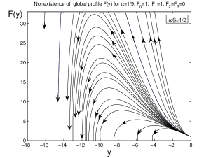
(a) $F_{1}=-1,\,F_{2}=F_{3}=0$

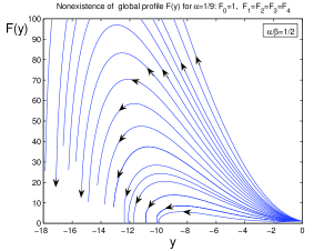
(b) $F_{1}=F_{2}=F_{3}=F_{4}$

Figure 16. Unsuccessful examples of 1D shooting of $F(y)$ of (5.6) from $y=0^{-}$.

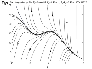
Figure 17. Unsuccessful 1D shooting of $F(y)$ satisfying (5.6) from $y=0^{-}$, with conditions $F(0)=1$, $F^{\prime}(0)=-1$, $F^{\prime\prime}(0)=F^{(4)}(0)=0$, and $F^{\prime\prime\prime}(0)=-0.2000223777...$ being a parameter.

Therefore, we now use the bvp4c solver, and this gives the following results for the case (5.27), with $C_{0}=1$, as usual. Namely, we show that there are two parameters, say,

(5.38) $$F_{0}=F(0)\quad\mbox{and}\quad F_{1}=F^{\prime}(0),$$

such that, for their arbitrary values from some connected subset in $\mathbb{R}^{2}$, including all points with $F_{0}>0$ and $F_{1}\leq 0$, the problem (5.6) admits a solution. This is confirmed in Figure 18 for the case $F^{\prime}(0)=0$ and in Figure 19 for the cases $F^{\prime}(0)=+1$ (a) and $F^{\prime}(0)=-1$ (b). Obviously, all these profiles are different and exhibit fast and “non-oscillatory” convergence as $y\to-\infty$ to the “good” bundle as in (5.6) with $C_{0}=1$.

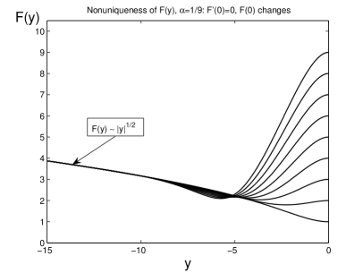
Figure 18. Global profiles $F(y)$ of (5.6) for $\alpha=\frac{1}{9}$, $C_{0}=1$, $F^{\prime}(0)=0$; $F(0)\in[1,9]$ being a parameter.

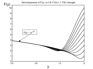
(a) $F^{\prime}(0)=+1$

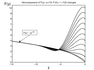
(b) $F^{\prime}(0)=-1$

Figure 19. Global profiles $F(y)$ of (5.6) for $\alpha=\frac{1}{9}$, $C_{0}=1$ and $F^{\prime}(0)=+1$ (a), $F^{\prime}(0)=-1$ (b); $F(0)\in[0,10]$ being a parameter.

Finally, carefully analyzing the dimensions of all the “bad” and “good” asymptotic bundles indicated in (i) and (ii) above, plus (5.37), unlike the result for blow-up profiles in Proposition 5.1, we arrive at even stronger nonuniqueness:

Proposition 5.2.

In the range $(\ref{Ran1})$ and any fixed $C_{0}>0$, the problem $(\ref{s2Na})$ admits a $2$D family of solutions, which can be parameterized by $F_{0}$ and $F_{1}$.

Recall again that, for any hope of uniqueness, the extension pair $\{f,F\}$ must be unique (or at least their subset should contain some “minimal” and/or isolated points as proper candidates for unique entropy solutions) for any fixed constant $C_{0}>0$, which defines the “initial data” (5.3) at the blow-up time $t=0^{-}$. This actually happens for the Euler equation (1.7); see [21, § 4], where the similarity analysis is indeed easier and is reduced to algebraic manipulations, but not that straightforward anyway even for such a “first-order NDE”.

5.5. “Initial nonuniqueness”

A new “nonuniqueness” phenomenon is achieved for the values of parameters

(5.39) $$F(0)=F_{0}<0\quad\mbox{and}\quad F^{\prime}(0)=F_{1}\geq 0.$$

Figure 20(a), (b) shows such shock profiles leading to the nonuniqueness, obtained by a standard 1D shooting via the ode45 solver. Here, two similarity profiles $F(y)$ are obtained via distinct types of shooting: relative to the parameter $F^{\prime}(0)=F^{\prime\prime\prime}(0)$ in (a), and relative $F_{2}(0)$ in (b).

The proof of existence of such profiles $F$ is based on the same geometric arguments as that of Proposition 2.3 (with the evident change of the geometry of the phase space). These two different profiles posed into the similarity solutions (5.5) show a nonunique way to get solutions with initial data ($C_{0}=1$ by scaling) at $t=0^{+}$:

(5.40) $$u_{0}(x)=|x|^{\frac{\alpha}{\beta}}{\rm sign}\,x\quad\mbox{in}\quad\mathbb{R},$$

which already have a gradient blow-up singularity at $x=0$. This is another potential type of nonuniqueness in the Cauchy problem for (1.5), showing the nonunique way of formation of shocks from weak discontinuities, including the stationary ones as in (5.29).

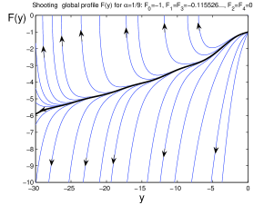
(a) $F^{\prime}(0)=F^{\prime\prime\prime}(0)=-0.115526...$

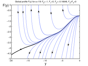
(b) $F^{\prime}(0)=0,\,\,F^{\prime\prime}(0)=-0.16648...$

Figure 20. Shooting a proper solution $F(y)$ of (5.6) for $\alpha=\frac{1}{9}$ with data $F(0)=-1$, $F_{4}=0$, and $F^{\prime}(0)=F^{\prime\prime\prime}(0)=-0.115526...$ (shooting parameter), $F_{2}=0$ (a), and $F(0)=-1$, $F^{\prime}(0)=0$, $F_{2}=-0.16648...\,$ (shooting parameter), $F_{3}=F_{4}=0$ (b).

However, bearing in mind Proposition 4.2 saying that the shocks of $S_{+}$-type are not $\delta$-entropy (i.e., not stable relative small smooth deformations), one can expect that the shocks as in (5.39) are also unstable. Indeed, smooth extensions of weak pointwise shocks (5.40) via rarefaction self-similar waves given by (5.6) are $\delta$-entropy. In Figure 21, we show such a global rarefaction profile $F(y)$ for $\alpha=\frac{1}{9}$, which describes smooth collapse of the “weak equilibrium” (5.29). One can see that such rarefaction profiles satisfy $F(y)\equiv-f(y)$, where $f$ are the corresponding blow-up ones, as shown in Figure 12 for various $\alpha$.

Overall, it seems that the $\delta$-entropy test rules out such an “initial nonuniqueness” with data of type $S_{+}$ as in (5.40), where a unique smooth rarefaction extension is available. On the other hand, for other classes of data of $S_{-}$-shape (according to Proposition 4.1), such a nonuniqueness can take place; see Section 5.4.

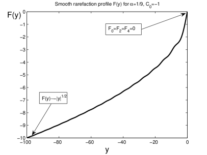
Figure 21. Global rarefaction profile $F(y)$ of (5.6) for $\alpha=\frac{1}{9}$, $C_{0}=-1$; $F(0)=F^{\prime\prime}(0)=F^{(4)}(0)=0$.

5.6. More on nonuniqueness and well-posedness of FBPs

The nonuniqueness (5.8) in the Cauchy problem (1.5), (5.3) is as follows: any $F(y)$ yields the self-similar continuation (5.5), with the behaviour of the jump at $x=0$ (profiles $F(y)$ as in Figure 20)

(5.41) $$-[u_{+}(x,t)]\big{|}_{x=0}\equiv-\big{(}u_{+}(0^{+},t)-u_{+}(0^{-},t))=2F_{0}t^{\alpha}<0\quad\mbox{for}\quad t>0.$$

In the similarity ODE representation, this nonuniqueness has a pure geometric-dimensional origin associated with the dimension and mutual geometry of the good and bad asymptotic bundles of the 5D phase spaces of both blow-up and global equations. Since these shocks are stationary, the corresponding Rankine–Hugoniot (R–H) condition on the speed $\lambda$ of the shock propagation:

(5.42) $$\lambda=\frac{[(uu_{x})_{xxx}]}{[u]}\big{|}_{x=0}\equiv\frac{[(u^{2})_{xxxx}]}{2[u]}\big{|}_{x=0}=\frac{[(f^{2})^{(4)}]}{2[f]}\big{|}_{y=0}=0$$

is valid by anti-symmetry. As usual, (5.42) is obtained by integration of the equation (1.30) in a small neighbourhood of the shock. The R–H condition does not assume any novelty and is a corollary of integrating the PDE about the line of discontinuity.

Moreover, the R–H condition (5.42) also indicates another origin of nonuniqueness: a symmetry breaking. Indeed, the solution for $t>0$ is not obliged to be an odd function of $x$, so the self-similar solution (5.5) for $x<0$ and $x>0$ can be defined using ten different parameters $\{F_{0}^{\pm},...,F_{4}^{\pm}\}$, and the only extra condition one needs is the R–H one:

(5.43) $$[(FF^{\prime})^{\prime\prime\prime}](0)=0,\quad\mbox{i.e.,}\quad F_{0}^{-}F_{4}^{-}+4F_{1}^{-}F_{3}^{-}+3(F_{2}^{-})^{2}=F_{0}^{+}F_{4}^{+}+4F_{1}^{+}F_{3}^{+}+3(F_{2}^{+})^{2}.$$

This algebraic equations with ten unknowns admit many other solutions rather than the obvious anti-symmetric one:

$$F_{0}^{-}=-F_{0}^{+},\quad F_{1}^{-}=F_{1}^{+},\quad F_{2}^{-}=-F_{2}^{+},\quad F_{3}^{-}=F_{3}^{+},\,\,\,\mbox{and}\,\,\,F_{4}^{-}=-F_{4}^{+}.$$

Finally, we note that the uniqueness can be restored by posing specially designed conditions on moving shocks, which, overall guarantee the unique solvability of the algebraic equation in (5.43) and hence the unique continuation of the solution beyond blow-up. This construction is analytically similar to that for the NDEs–3 (1.30) in [21].

6. Shocks for an NDE obeying the Cauchy–Kovalevskaya theorem

In this short section, we touch on the problem of formation of shocks for NDEs that are higher-order in time. Instead of studying the PDEs such as (cf. [18, 23])

(6.1) $$u_{tt}=-(uu_{x})_{xxxx},\quad u_{ttt}=-(uu_{x})_{xxxx},\quad\mbox{etc.},$$

we consider the fifth-order in time NDE (1.11), which exhibits certain simple and, at the same time, exceptional properties. Writing it for $W=(u,v,w,g,h)^{T}$ as

(6.2) $$\left\{\begin{matrix}u_{t}=v_{x},\,\,\,\,\,\,\\ v_{t}=w_{x},\,\,\,\,\,\\ w_{t}=g_{x},\,\,\,\,\,\\ g_{t}=h_{x},\,\,\,\,\,\\ h_{t}=uu_{x},\end{matrix}\right.\quad\mbox{or}\quad W_{t}=AW_{x},\quad\mbox{with the matrix}\quad A=\left[\begin{matrix}0\,\,\,1\,\,\,0\,\,\,0\,\,\,0\\ 0\,\,\,0\,\,\,1\,\,\,0\,\,\,0\\ 0\,\,\,0\,\,\,0\,\,\,1\,\,\,0\\ 0\,\,\,0\,\,\,0\,\,\,0\,\,\,1\\ u\,\,\,0\,\,\,0\,\,\,0\,\,\,0\end{matrix}\right],$$

(1.11) becomes a first-order system with the characteristic equation for eigenvalues

$$-\lambda^{5}+u=0.$$

Hence, for any $u\not=0$, there exist complex roots, so that advanced results on hyperbolic systems [1, 10] cannot be applied.

6.1. Evolution formation of shocks

For (1.11), the blow-up similarity solution is

(6.3) $$u_{-}(x,t)=g(z),\quad z=x/(-t),\quad\mbox{where}$$

(6.4) $$\begin{matrix}(gg^{\prime})^{(4)}=(z^{5}g^{\prime})^{(4)}\equiv 120g^{\prime}z+240g^{\prime\prime}z^{2}+120g^{\prime\prime\prime}z^{3}\vskip 3.0pt plus 1.0pt minus 1.0pt\vskip 3.0pt plus 1.0pt minus 1.0pt\vskip 3.0pt plus 1.0pt minus 1.0pt\\ +20g^{(4)}z^{4}+g^{(5)}z^{5}\quad\mbox{in}\quad\mathbb{R},\quad f(\mp\infty)=\pm 1.\end{matrix}$$

Integrating (6.4) four times yields

(6.5) $$gg^{\prime}=z^{5}g^{\prime}+Az+Bz^{3},\quad\mbox{with constants}\quad A=(g^{\prime}(0))^{2}>0,\,\,B=\frac{2}{3}\,g^{\prime}(0)g^{\prime\prime\prime}(0),$$

so that the necessary similarity profile $g(z)$ solves the first-order ODE

(6.6) $$\frac{{\mathrm{d}}g}{{\mathrm{d}}z}=\frac{Az+Bz^{3}}{g-z^{5}}.$$

By the phase-plane analysis of (6.6) with $A>0$ and $B=0$, we easily get the following:

Proposition 6.1.

The problem $(\ref{2.2tt})$ admits a solution $g(z)$ satisfying the anti-symmetry conditions $(\ref{2.4})$ that is positive for $z<0$, monotone decreasing, and is real analytic.

Actually, involving the second parameter $B>0$ yields that there exist infinitely many shock similarity profiles. The boldface profile $g(z)$ in Figure 22 (by (6.3), it gives $S_{-}(x)$ as $t\to 0^{-}$) is non-oscillatory about $\pm 1$, with the following algebraic rate of convergence to the equilibrium as $z\to-\infty$:

$$g(z)=\left\{\begin{matrix}1+\frac{A}{3z^{5}}+...\,\,\,\mbox{for}\,\,\,B=0,\vskip 3.0pt plus 1.0pt minus 1.0pt\\ 1+\frac{B}{z}+...\,\,\,\,\,\,\mbox{for}\,\,\,B>0.\end{matrix}\right.$$

Note that the fundamental solutions of the corresponding linear PDE

(6.7) $$u_{ttttt}=u_{xxxxx}$$

is also not oscillatory as $x\to\pm\infty$. This has the form

$$b(x,t)=t^{3}F(y),\quad y=x/t,\quad\mbox{so that}\,\,\,b(x,0)=...=b_{ttt}(x,0)=0,\,\,\,b_{tttt}(x,0)=\delta(x).$$

The linear equation (6.7) exhibits some features of finite propagation via TWs, since

$$u(x,t)=f(x-\lambda t)\quad\Longrightarrow\quad-\lambda^{5}f^{(5)}=f^{(5)},\,\,\,\,\mbox{i.e.,}\,\,\,\lambda=-1,$$

since the profile $f(y)$ disappears from the ODE. This is similar to some canonical equations of mathematical physics such as

$$u_{t}=u_{x}\,\,(\mbox{dispersion, $\lambda=-1$})\quad\mbox{and}\quad u_{tt}=u_{xx}\,\,(\mbox{wave equation, $\lambda=\pm 1$}).$$

The blow-up solution (6.3) gives in the limit $t\to 0^{-}$ the shock $S_{-}(x)$, and (1.8) holds.

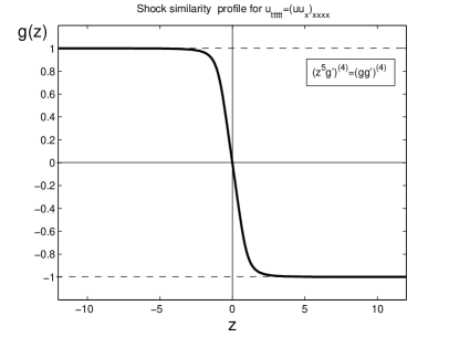
Figure 22. The shock similarity profile satisfying (6.4).

Since (1.11) has the same symmetry (3.1) as (1.30), similarity solutions (6.3), with $-t\mapsto t$ and $g(z)\mapsto g(-z)$ according to (3.5), also give the rarefaction waves for $S_{+}(x)$ as well as other types of collapse of initial non-entropy discontinuities.

6.2. Analytic $\delta$-deformations by Cauchy–Kovalevskaya theorem

The great advantage of the equation (1.11) is that it is in the normal form, so it obeys the Cauchy–Kovalevskaya theorem [53, p. 387]. Hence, for any analytic initial data $u(x,0)$, $u_{t}(x,0)$, $u_{tt}(x,0)$, $u_{ttt}(x,0)$, and $u_{tttt}(x,0)$, there exists a unique local in time analytic solution $u(x,t)$. Thus, (1.11) generates a local semigroup of analytic solutions, and this makes it easier to deal with smooth $\delta$-deformations that are chosen to be analytic. This defines a special analytic $\delta$-entropy test for shock/rarefaction waves. On the other hand, such nonlinear PDEs can admit other (say, weak) solutions that are not analytic. Actually, Proposition 6.1 shows that the shock $S_{-}(x)$ is a $\delta$-entropy solution of (1.11), which is obtained by finite-time blow-up as $t\to 0^{-}$ from the analytic similarity solution (6.3).

6.3. On formation of single-point shocks and extension nonuniqueness

Similar to the analysis in Section 5, for the model (1.11) (and (6.1)), these assume studying extension similarity pairs $\{f,F\}$ induced by the easy derived analogies of the blow-up (5.2) and global (5.6), with

$$\beta=\frac{5+\alpha}{5},$$

5D dynamical systems. These are very difficult, so that checking three types (standard, backward, and initial) of possible nonuniqueness and non-entropy of such flows with strong and weak shocks becomes a hard open problem, though some auxiliary analytic steps towards nonuniqueness are doable. Overall, in view of complicated multi-dimensional phase spaces involved, we do not have any reason for having a unique continuation after singularity. In other words, for such higher-order NDEs, uniqueness can occur accidentally only for very special phase spaces, and hence, at least, is not robust (in a natural ODE–PDE sense) anyway.

7. (V) Problem “Oscillatory Smooth Compactons” of fifth-order NDEs

We begin with an easier explicit example of nonnegative compactons for a third-order NDE.

7.1. Third-order NDEs: $\delta$-entropy compactons

Compactons as compactly supported TW solutions of the $K(2,2)$ equation (1.22) were introduced in 1993, [47], as

(7.1) $$u_{\rm c}(x,t)=f_{\rm c}(y),\,\,\,y=x+t\quad\Longrightarrow\quad f_{\rm c}:\quad f=(f^{2})^{\prime\prime}+f^{2}.$$

Integrating yields the following explicit compacton profile:

(7.2) $$f_{\rm c}(y)=\left\{\begin{matrix}\frac{4}{3}\cos^{2}\big{(}\frac{y}{4}\big{)}\quad\mbox{for}\quad|y|\leq 2\pi,\\ \qquad\,\,\,0\qquad\,\mbox{for}\quad|y|\geq 2\pi.\end{matrix}\right.$$

The corresponding compacton (7.1), (7.2) is G-admissible in the sense of Gel’fand (1959) [26, §§ 2, 8], and is a $\delta$-entropy solution [18, § 4], i.e., can be constructed by smooth (and moreover analytic) approximation via strictly positive solutions of the full third-order ODE for $f_{\rm c}(y)$ ,

$$f^{\prime}=(f^{2})^{\prime\prime\prime}+(f^{2})^{\prime}.$$

Since the PDE is not involved unlike Section 4.5, the $\delta$-entropy notion coincides with the G-admissability.

It is curious that the same compactly supported blow-up patterns occur in the combustion problem for the related reaction-diffusion parabolic equation

(7.3) $$u_{t}=(u^{2})_{xx}+u^{2}.$$

Then the standing-wave blow-up (as $t\to T^{-}$) solution of S-regime leads to the same ODE:

(7.4) $$u_{\rm S}(x,t)=(T-t)^{-1}f(x)\quad\Longrightarrow\quad f=(f^{2})^{\prime\prime}+f^{2}.$$

This yields the Zmitrenko–Kurdyumov blow-up localized solution, which has been known since 1975; see more historical details in [24, § 4.2].

7.2. Examples of $C^{3}$-smooth nonnegative compacton for higher-order NDEs

Such an example was given in [11, p. 4734]. Following [24, p. 189], we construct this explicit solution as follows. The operator ${\bf F}_{5}(u)$ of the quintic NDE

(7.5) $$u_{t}={\bf F}_{5}(u)\equiv(u^{2})_{xxxxx}+25(u^{2})_{xxx}+144(u^{2})_{x}$$

is shown to preserve the 5D invariant subspace

(7.6) $$W_{5}={\rm Span}\{1,\cos x,\sin x,\cos 2x,\sin 2x\},$$

i.e., ${\bf F}_{5}(W_{5})\subseteq W_{5}$. Therefore, (7.5) restricted to the invariant subspace $W_{5}$ is a 5D dynamical system for the expansion coefficients of the solution

$$u(x,t)=C_{1}(t)+C_{2}(t)\cos x+C_{3}(t)\sin x+C_{4}(t)\cos 2x+C_{5}(t)\sin 2x\in W_{5}.$$

Solving this yields the explicit compacton TW

(7.7) $$u_{\rm c}(x,t)=f_{\rm c}(x+t),\quad\mbox{where}\quad f_{\rm c}(y)=\left\{\begin{matrix}\frac{1}{105}\,\cos^{4}\bigl{(}\frac{y}{2}\bigr{)}\,\,\,\mbox{for}\,\,\,|y|\leq\pi,\vskip 3.0pt plus 1.0pt minus 1.0pt\\ \qquad\quad 0\qquad\mbox{for}\,\,\,|y|\geq\pi.\end{matrix}\right.$$

This $C^{3}_{x}$ solution can be attributed to the Cauchy problem for (7.5) since smooth solutions are not oscillatory near interfaces; see a discussion around [24, p. 184].

The above invariant subspace analysis applies also to the 7th-order PDE

(7.8) $$u_{t}={\bf F}_{7}(u)\equiv D_{x}^{7}(u^{2})+\beta D_{x}^{5}(u^{2})+\gamma(u^{2})_{xxx}+\nu(u^{2})_{x}.$$

Here ${\bf F}_{7}$ admits $W_{5}$ if

$$\mbox{ $\beta=25$, \,\,$\gamma=144$,\,\, and $\nu=0$}.$$

Moreover [24, p. 190], the only operator ${\bf F}_{7}$ in (7.8) preserving the 7D subspace

(7.9) $$W_{7}={\mathcal{L}}\{1,\cos x,\sin x,\cos 2x,\sin 2x,\cos 3x,\sin 3x\}$$

is in the following NDE–7:

(7.10) $$u_{t}={\bf F}_{7}(u)\equiv D_{x}^{7}(u^{2})+77D_{x}^{5}(u^{2})+1876(u^{2})_{xxx}+14400(u^{2})_{x}.$$

This makes it possible to reduce (7.10) on $W_{7}$ to a complicated dynamical system.

7.3. Why nonnegative compactons for fifth-order NDEs are not robust: a saddle-saddle homoclinic

Recall that, as usual in dynamical system theory, by robustness of trajectories we mean that these are stable with respect to small perturbations of the parameters entering the NDE or the corresponding ODEs. In other words, the dynamical systems (ODEs) admitting such non-negative “heteroclinic” saddle-like orbits $0\to 0$ are not structurally stable in a natural sense. This reminds the classic Andronov–Pontriagin–Peixoto theorem, where one of the four conditions for the structural stability of dynamical systems in $\mathbb{R}^{2}$ reads as follows [38, p. 301]:

(7.11) “(ii) there are no trajectories connecting saddle points… .”

Actually, nonnegative compactons, such as (7.7), are special homoclinics of the origin, and we will show that the nature of their non-robustness is in the fact that these represent a stable-unstable manifold of the origin consisting of a single orbit. Therefore, in consistency with (7.11), the origin is indeed a saddle in $\mathbb{R}^{4}$ in the plane $\{f,f^{\prime},f^{\prime\prime},f^{\prime\prime\prime}\}$, obtained after integration once; see below.

In order to illustrate the lack of such a robustness in view of a sole heteroclinic involved, consider the NDE (7.5), for which, substituting the TW solution, on integration, we obtain the following ODE:

(7.12) $$u_{\rm c}(x,t)=f_{\rm c}(x+t)\quad\Longrightarrow\quad f_{\rm c}:\quad 2f=(f^{2})^{(4)}+...\,,$$

where we omit the lower-order terms as $f\to 0$. Looking for the compacton profile $f\geq 0$, we set $f^{2}=F$ to get

(7.13) $$F^{(4)}=2\sqrt{F}+...\quad\mbox{for}\quad y>0,\quad F^{\prime}(0)=F^{\prime\prime\prime}(0)=0.$$

As usual, we look for a symmetric $F(y)$ by putting two symmetry conditions at the origin.

Let $y=y_{0}>0$ be the interface point of $F(y)$. Then, looking for the expansion as $y\to y_{0}^{-}$ in the form

(7.14) $$F(y)=\frac{1}{840^{2}}\,(y_{0}-y)^{8}+\varepsilon(y),\quad\mbox{with}\quad\varepsilon(y)=o((y_{0}-y)^{8}),$$

we obtain Euler’s equation for the perturbation $\varepsilon(y)$,

(7.15) $$\frac{1}{840}(y_{0}-y)^{4}\varepsilon^{(4)}-\varepsilon=0.$$

Hence, $\varepsilon(y)=(y_{0}-y)^{m}$, with the characteristic equation

(7.16) $$m(m-1)(m-2)(m-3)-840=0\,\Longrightarrow\,m_{1}=-4,\,\,\,m_{2,3}=\frac{3\pm{\rm i}\sqrt{111}}{2},\quad m_{4}=7.$$

Hence, ${\rm Re}\,m_{i}<8$, and, in other words, (7.15) does not admit any nontrivial solution satisfying the condition in (7.14); see further comments in [24, p. 142]. In fact, it is easy to see that (7.15) with $\varepsilon=0$ is the unique positive smooth solution of $F^{(4)}=2\sqrt{F}$. Thus,

(7.17) $$\mbox{the asymptotic bundle of solutions (\ref{gg3}) is 1D},$$

where the only parameter is the position of the interface $y_{0}>0$.

Obviously, as a typical property, this 1D bundle is not sufficient to satisfy (by shooting) two conditions at the origin in (7.13), so such TW profiles $F(y)\geq 0$ are nonexistent for almost all NDEs like that. In other words, the condition of positivity of the solution,

(7.18) to look for a nontrivial solution $$F\geq 0$$ for the ODE in (7.13)

creates a free-boundary “obstacle” problem that, in general, is inconsistent. Skipping the obstacle condition (7.18) will return such ODEs (or elliptic equations), with a special extension, into the consistent variety, as we will illustrate below.

Thus, nonnegative TW compactons are not generic (robust) solutions of $(2m+1)$th-order quadratic NDEs with $m=2$, and also for larger $m$’s, where some kind of (7.17), as a “dimensional defect” (the bundle dimension is smaller than the number of conditions at $y=0$ to shoot), remains valid.

7.4. Nonnegative compactons are robust for third-order NDEs only

The third-order case $m=1$, i.e., NDEs such as (1.22), is the only one where propagation of perturbations via nonnegative TW compactons is structurally stable, i.e., with respect to small perturbation of the parameters (and nonlinearities) of equations. Mathematically speaking, then the 1D bundle in (7.17) perfectly matches with the single symmetry condition at the origin,

$$F^{\prime\prime}=2\sqrt{F}+...\quad\mbox{and}\quad F^{\prime}(0)=0.$$

7.5. Compactons of changing sign are robust and $\delta$-entropy for the NDEs–5

As a typical example, we consider the perturbed version (1.12) of the NDE–(1,4) (1.5). As we have mentioned, this is is written for solutions of changing sign, since nonnegative compactons do not exist in general. Looking for the TW compacton (7.12) yields the ODE

(7.19) $$f=-\frac{1}{2}\,(|f|f)^{(4)}+\frac{1}{2}\,|f|f\quad\Longrightarrow\quad F^{(4)}=F-2|F|^{-\frac{1}{2}}F\,\,\,\mbox{for}\,\,\,F=|f|f.$$

Such ODEs with non-Lipschitz nonlinearities are known to admit countable sets of compactly supported solutions, which are studied by a combination of Lusternik–Schnirel’man and Pohozaev’s fibering theory; see [22].

In Figure 23, we present the first TW compacton patterns (the boldface line) and the second one that is essentially non-monotone. These look like standard compacton profiles but careful analysis of the behaviour near the finite interface at $y=y_{0}$ shows that $F(y)$ changes sign infinitely many times according to the asymptotics

(7.20) $$F(y)=(y_{0}-y)^{8}[\varphi(s+s_{0})+o(1)],\,\,\,s=\ln(y_{0}-y)\quad\mbox{as}\quad y\to y_{0}^{-}.$$

Here, the oscillatory component $\varphi(s)$ is a periodic solution of a certain nonlinear ODE and $s_{0}$ is an arbitrary phase shift; see [24, § 4.3] and [22, § 4] for further details. Thus, unlike (7.17),

(7.21) $$\mbox{the asymptotic bundle of solutions (\ref{z4}) is 2D (parameters are $y_{0}$ and $s_{0}$)},$$

and exhibits some features of a “nonlinear focus” (not a saddle as above) on some manifold. Hence, this is enough to match also two symmetry boundary conditions given in (7.13). Such a robust solvability is confirmed by variational techniques that apply to rather arbitrary equations such as in (7.19) with similar singular non-Lipschitz nonlinearities.

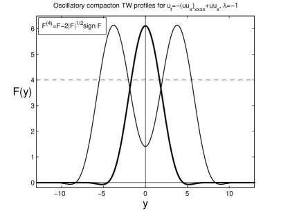
Figure 23. First two compacton TW profiles $F(y)$ satisfying the ODE in (7.19).

Let us also note that such oscillatory compactons are also $\delta$-entropy in the sense that can be approximated by analytic TW solutions of the same ODE but having finite number of zeros (i.e., admit smooth analytic $\delta$-deformations); see [18, § 8.3] for a related NDE–5.

Regardless the existence of such sufficiently smooth compacton solutions, it is worth recalling again that, for the NDE (1.12), as well as (2.35) and (4.3), both containing monotone nonlinearities, the generic behaviour, for other initial data, can include formation of shocks in finite time, with the local similarity mechanism as in Section 2 and in Section 5.1, representing more generic single point shock pattern formations.

8. Final conclusions

The fifth-order nonlinear dispersion equations (1.1)–(1.5) (NDEs–5), which are associated with a number of important applications, are considered. The main achieved properties of such 1D degenerate nonlinear PDEs are as follows:

(i) Section 2: these NDEs admit blow-up self-similar formation from smooth solutions of shock waves of a specific oscillatory structure, which correspond to initial data $S_{-}(x)=-{\rm sign}\,x$, i.e., the same as for the first-order conservation law (1.30);

(ii) Section 3: as customary, self-similar rarefaction waves, which get smooth for any $t>0$, are created by the reversed data $S_{+}(x)={\rm sign}\,x$;

(iii) Unlike the classical theory of first-order conservation laws developed in the 1950s–60s, the entropy-type techniques are no longer applied for distinguishing general proper (unique) solutions. A $\delta$-deformation test via smoothing the solutions is developed in Section 4, which is able to separate shocks and rarefaction waves for particular classes of initial data $\sim S_{\pm}(x)$ with a simple geometry of initial shocks;

(iv) Section 5: by studying more general self-similar solutions of NDEs, it was shown that uniqueness of the solutions after formation of a shock is principally impossible. Namely, there exist single point gradient blow-up similarity solutions, which admit an infinite number of self-similar extensions beyond. This 2D set of shock wave extensions after singularity does not have any distinguished solutions (say, maximal, minimal, isolated, etc.). This also suggests that any entropy-like mechanisms for a unique continuation do not exist either. However, using a proper free-boundary setting, i.e., posing special conditions on shocks, can restore uniqueness; and

(v) Section 7: nonnegative compacton solutions for some NDEs–5 are shown to be non-robust (not “structurally stable”), i.e., these disappear after a.a. arbitrarily small perturbations of the parameters (nonlinearities) of the equations. However, oscillatory compactons of changing sign near finite interface are shown to exist and to be robust.

Acknowledgements. The authors would like to thank the anonymous Referee from the European Journal of Applied Mathematics for an extremely useful discussion concerning $\delta$-deformation issues for shock/rarefaction waves.

References

- [1] A. Bressan, Hyperbolic Systems of Conservation Laws. The One Dimensional Cauchy Problem, Oxford Univ. Press, Oxford, 2000.
- [2] H. Cai, Dispersive smoothing effects for KdV type equations, J. Differ. Equat., 136 (1997), 191–221.
- [3] D. Christodoulou,The Euler equations of compressible fluid flow, Bull. Amer. Math. Soc., 44 (2007), 581–602.
- [4] P.A. Clarkson, A.S. Fokas, and M. Ablowitz, Hodograph transformastions of linearizable partial differential equations, SIAM J. Appl. Math., 49 (1989), 1188–1209.
- [5] G.M. Coclite and K.H. Karlsen, On the well-posedness of the Degasperis–Procesi equation, J. Funct. Anal., 233 (2006), 60–91.
- [6] O. Costin and S. Tanveer, Complex singularity analysis for a nonlinear PDE, Commun. Part. Differ. Equat., 31 (2006), 593–637.
- [7] W. Craig and J. Goodman, Linear dispersive equations of Airy type, J. Differ. Equat., 87 (1990), 38–61.
- [8] W. Craig, T. Kappeler, and W. Strauss, Gain of regularity for equations of KdV type, Ann. Inst. H. Poincare, 9 (1992), 147–186.
- [9] G. Da Prato and P. Grisvard, Equation d’évolutions abstraites de type parabolique, Ann. Mat. Pura Appl., IV(120) (1979), 329–396.
- [10] C. Dafermos, Hyperbolic Conservation Laws in Continuum Physics, Springer-Verlag, Berlin, 1999.
- [11] B. Dey, Compacton solutions for a class of two parameter generalized odd-order Korteweg–de Vries equations, Phys. Rev. E, 57 (1998), 4733–4738.
- [12] L.L. Dawson, Uniqueness properties of higher order dispersive equations, J. Differ. Equat., 236 (2007), 199–236.
- [13] Yu.V. Egorov, V.A. Galaktionov, V.A. Kondratiev, and S.I. Pohozaev, Asymptotic behaviour of global solutions to higher-order semilinear parabolic equations in the supercritical range, Adv. Differ. Equat., 9 (2004), 1009–1038.
- [14] J. Escher, Y. Liu, and Z. Yin Shock waves and blow-up phenomena for the periodic Degasperis–Procesi equation, Indiana Univ. Math. J., 56 (2007), 87–117.
- [15] J. Escher and G. Prokert, Analyticity of solutions to nonlinear parabolic equations on manifolds and an application to Stokes flow, J. Math. Fluid Mech., 8 (2006), 1–35.
- [16] A.V. Faminskii, On the mixed problem for quasilinear equations of the third order, J. Math. Sci., 110 (2002), 2476–2507.
- [17] V.A. Galaktionov, Sturmian nodal set analysis for higher-order parabolic equations and applications, Adv. Differ. Equat., 12 (2007), 669–720.
- [18] V.A. Galaktionov, Nonlinear dispersive equations: smooth deformations, compactons, and extensions to higher orders, Comput. Math. Math. Phys., 48 (2008), 1823–1856 (arXiv:0902.0275).
- [19] V.A. Galaktionov, Shocks waves and compactons for fifth-order nonlinear dispersion equations, arXiv:0902.1632.
- [20] V.A. Galaktionov, On regularity of a boundary point in higher-order parabolic equations: towards Petrovskii-type criterion by blow-up approach, NoDEA, 16 (2009), 597–655 (arXiv:0901.3986).
- [21] V.A. Galaktionov, On single point gradient blow-up and nonuniqueness for a third-order nonlinear dispersion equation, submitted; see arXiv.org.
- [22] V.A. Galaktionov, E. Mitidieri, and S.I. Pohozaev, Variational approach to complicated similarity solutions of higher-order nonlinear evolution equations of parabolic, hyperbolic, and nonlinear dispersion types, In: Sobolev Spaces in Mathematics. II, Appl. Anal. and Part. Differ. Equat., Series: Int. Math. Ser., Vol. 9, V. Maz’ya Ed., Springer, New York, 2009 (an earlier preprint in: arXiv:0902.1425).
- [23] V.A. Galaktionov and S.I. Pohozaev, Third-order nonlinear dispersive equations: shocks, rarefaction, and blow-up waves, Comput. Math. Math. Phys., 48 (2008), 1784–1810 (arXiv:0902.0253).
- [24] V.A. Galaktionov and S.R. Svirshchevskii, Exact Solutions and Invariant Subspaces of Nonlinear Partial Differential Equations in Mechanics and Physics, ChapmanHall/CRC, Boca Raton, Florida, 2007.
- [25] F. Gazzola and H.-C. Grunau, Radial entire solutions for supercritical biharmonic equations, Math. Ann., 334 (2006), 905–936.
- [26] I.M. Gel’fand, Some problems in the theory of quasilinear equations, Uspekhi Mat. Nauk., 14 (1959), 87–158; Amer. Math. Soc. Transl. (2), 29 (1963), 295–381.
- [27] T. Hoshiro, Mouree’s method and smoothing properties of dispersive equations, Comm. Math. Phys., 202 (1999), 255–265.
- [28] J.M. Hyman and P. Rosenau, Pulsating multiplet solutions of quintic wave equations, Phys. D, 123 (1998), 502–512.
- [29] M. Inc, New compacton and solitary pattern solutions of the nonlinear modified dispersive Klein–Gordon equations, Chaos, Solitons and Fractals, 33 (2007), 1275–1284.
- [30] S. Kawamoto, An exact transformation from the Harry Dym equation to the modified KdV equation, J. Phys. Soc. Japan, 54 (1985), 2055–2056.
- [31] S.N. Kruzhkov, First-order quasilinear equations in several independent variables, Math. USSR Sbornik, 10 (1970), 217–243.
- [32] H. Landmark, Formation and dynamiocs of shock waves in the Degasperis–Procesi equation, J. Nonl. Sci., 17 (2007), 169–198.
- [33] J.L. Levandosky, Smoothing properties of nonlinear dispersive equations in two spatial dimensions, J. Differ. Equat., 175 (2001), 275–372.
- [34] A. Lunardi, Analytic Semigroups and Optimal Regularity in Parabolic Problems, Birkhäuser, Basel/Berlin, 1995.
- [35] M.A. Naimark, Linear Differential Operators, Part I, Ungar Publ. Comp., New York, 1968.
- [36] O.A. Oleinik, Discontinuous solutions of non-linear differential equations, Uspehi Mat. Nauk., 12 (1957), 3–73; Amer. Math. Soc. Transl. (2), 26 (1963), 95–172.
- [37] O.A. Oleinik, Uniqueness and stability of the generalized solution of the Cauchy problem for a quasi-linear equation, Uspehi Mat. Nauk., 14 (1959), 165–170; Amer. Math. Soc. Transl. (2), 33 (1963), 285–290.
- [38] L. Perko, Differential Equations and Dynamical Systems, Springer-Verlag, New York, 1991.
- [39] D. Poisson, Mémoire sur la théorie du son, J. Polytech. (14 éme cahier) 7 (1808), 319–392.
- [40] Y. Pomeau, M. Le Berre, P. Guyenne, and S. Grilli, Wave-breaking and generic singularities of nonlinear hyperbolic equations, Nonlinearity, 21 (2008), T61–T79.
- [41] A.V. Porubov and M.G. Velarde, Strain kinks in an elastic rod embedded in a viscoelastic medium, Wave Motion, 35 (2002), 189–204.
- [42] B. Riemann,Über die Fortpfanzung ebener Luftwellen von endlicher Schwingungswete, Abhandlungen der Gesellshaft der Wissenshaften zu Göttingen, Meathematisch-physikalishe Klasse, 8 (1858-59), 43.
- [43] P. Rosenau, Nonlinear dispertion and compact structures, Phys. Rev. Lett., 73 (1994), 1737–1741.
- [44] P. Rosenau, On solitons, compactons, and Lagrange maps, Phys. Lett. A, 211 (1996), 265–275.
- [45] P. Rosenau, On a class of nonlinear dispersive-dissipative interactions, Phys. D, 123 (1998), 525–546.
- [46] P. Rosenau, Compact and noncompact dispersive patterns, Phys. Lett. A, 275 (2000), 193–203.
- [47] P. Rosenau and J.M. Hyman, Compactons: solitons with finite wavelength, Phys. Rev. Lett., 70 (1993), 564–567.
- [48] P. Rosenau and S. Kamin, Thermal waves in an absorbing and convecting medium, Phys. D, 8 (1983), 273–283.
- [49] P. Rosenau and D. Levy, Compactons in a class of nonlinearly quintic equations, Phys. Lett. A, 252 (1999), 297–306.
- [50] J. Smoller, Shock Waves and Reaction-Diffusion Equations, Springer-Verlag, New York, 1983.
- [51] H. Takuwa, Microlocal analytic smoothing effects for operators of real principal type, Osaka J. Math., 43 (2006), 13–62.
- [52] T. Tao, Multilinear weighted convolution of functions, and applications to nonlinear dispersive equations, Amer. J. Math., 6 (2000), 839–908.
- [53] M.E. Taylor, Partial Differential Equations III. Nonlinear Equations, Springer-Verlag, New York, 1996.
- [54] Z. Yan, Constructing exact solutions for two-dimensional nonlinear dispersion Boussinesq equation II. Solitary pattern solutions, Chaos, Solitons and Fractals, 18 (2003), 869–880.
- [55] R.-X. Yao and Z.-B. Li, Conservation laws and new exact solutions for the generalized seventh order KdV equation, Chaos, Solitons and Fractals, 20 (2004), 259–266.