Dynamo Onset as a First-Order Transition: Lessons from a Shell Model for Magnetohydrodynamics

Abstract

We carry out systematic and high-resolution studies of dynamo action in a shell model for magnetohydrodynamic (MHD) turbulence over wide ranges of the magnetic Prandtl number $Pr_{\rm M}$ and the magnetic Reynolds number $Re_{\rm M}$. Our study suggests that it is natural to think of dynamo onset as a nonequilibrium, first-order phase transition between two different turbulent, but statistically steady, states. The ratio of the magnetic and kinetic energies is a convenient order parameter for this transition. By using this order parameter, we obtain the stability diagram (or nonequilibrium phase diagram) for dynamo formation in our MHD shell model in the $(Pr^{-1}_{\rm M},Re_{\rm M})$ plane. The dynamo boundary, which separates dynamo and no-dynamo regions, appears to have a fractal character. We obtain hysteretic behavior of the order parameter across this boundary and suggestions of nucleation-type phenomena.

I Introduction

The elucidation of dynamo action is a problem of central importance in nonlinear dynamics because it has implications for a variety of physical systems. Dynamo instabilities, which amplify weak magnetic fields in a turbulent conducting fluid, are believed to be the principal mechanism for the generation of magnetic fields in celestial bodies and in the interstellar medium arnab ; rudiger ; goedbloed ; biskamp ; mkvrev ; njpspecial ; schekochihin , and in liquid-metal systems roberts ; fauve ; riga ; karl ; lathrop ; pinton studied in laboratories. In these situations the kinematic viscosity $\nu$ and the magnetic diffusivity $\eta$ can differ by several orders of magnitude, so the magnetic Prandtl number $Pr_{\rm M}\equiv\nu/\eta$ can either be very small or very large; e.g., $Pr_{\rm M}\simeq 10^{-2}$ at the base of the Sun’s convection zone, $Pr_{\rm M}\simeq 10^{-5}$ in the liquid-sodium system, and $Pr_{\rm M}\simeq 10^{14}$ in the interstellar medium. This Prandtl number is related to the Reynolds number $Re=UL/\nu$ and the magnetic Reynolds number $Re_{\rm M}=UL/\eta$ that characterize the conducting fluid; here $L$ and $U$ are typical length and velocity scales in the flow; clearly $Pr_{\rm M}=Re_{\rm M}/Re$.

Two dissipative scales play an important role here; they are the Kolmogorov scale $\ell_{d}$ [$\sim\nu^{3/4}$ at the level of Kolmogorov 1941 (K41) phenomenology K41 ] and the magnetic-resistive scale $\ell_{d}^{M}$ [$\sim\eta^{3/4}$ in K41]. For large Prandtl numbers, i.e., $Pr_{\rm M}\gg 1$, $\ell_{d}^{M}\ll\ell_{d}$ so the magnetic field grows predominantly in the dissipation range of the fluid till it is strong enough to affect the dynamics of the fluid through the Lorentz force. This behavior is a characteristic of a small-scale turbulent dynamo, in which dynamo action is driven by a smooth, dissipative-scale velocity field. In the initial stage of growth, called the kinematic stage of the dynamo, the magnetic field is not large enough to act back on the velocity field. Dynamo action can be obtained for values of $Re_{\rm M}$ that are large enough to overcome Joule dissipation; and the dynamo-threshold value $Re_{\rm Mb}$ decreases as $Pr_{\rm M}$ increases boldyrev ; ponty . $Pr_{\rm M}\simeq 10^{-5}$ in liquid-metal flows riga ; pinton ; kenjeres so they lie in the small-Prandtl-number region, $Pr_{\rm M}\ll 1$, for which the growth of the magnetic energy occurs initially in the inertial scales of fluid turbulence, because $\ell_{d}\ll\ell_{d}^{M}$; here the velocity field is not smooth and the local strain rate is not uniform: At the K41 level the turnover velocity of an eddy of size $\ell$ is $v(\ell)\sim\ell^{1/3}$, so the rate of shearing $(v(\ell)/\ell)\sim\ell^{-2/3}$.

Direct numerical simulations (DNS) are playing an increasingly important role in developing an understanding of such dynamo action. Most DNS studies of MHD turbulence frisch ; chou ; ponty ; minnini have been restricted, because of computational constraints, either to low resolutions or to the case $Pr_{\rm M}=1$; small-scale dynamos, with $Pr_{\rm M}\gg 1$ have also been studied via DNS schekochihin . However, given the large range spanned by $Pr_{\rm M}$ in the physical settings mentioned above, some recent DNS studies of the MHD equations have started to explore the $Pr_{\rm M}$ dependence of dynamo action; the range of $Pr_{\rm M}$ covered by such pure DNS studies ponty ; brandenburgdns is quite modest ($10^{-2}\lesssim Pr_{\rm M}\lesssim 10$). To explore the dynamo boundary in the $(Pr^{-1}_{\rm M},Re_{\rm M})$ plane over a large range of $Pr_{\rm M}$, one recent study ponty has used a combination of numerical methods, some of which require small-scale models like large-eddy simulations (LES) or lagrangian-averaged MHD (LAMHD), and others, like a pseudospectral DNS, in which the only approximations are the finite number of collocation points and the finite step used in time marching; yet another DNS study iskakov has introduced hyperviscosity of order $8$ to study the low $Pr_{\rm M}$ regime; by using this combination of methods these studies has been able to cover the range $10^{-2}\lesssim Pr_{\rm M}\lesssim 10^{3}$ and to obtain the boundary between dynamo and no-dynamo regions but with fairly large error bars.

We have carried out extensive, high-resolution, numerical studies that have been designed to explore in detail the boundary between the dynamo and no-dynamo regimes in the $(Pr^{-1}_{\rm M},Re_{\rm M})$ plane in a shell model for three-dimensional MHD basu ; frick ; brandenburgshell ; giuliani . This shell model allows us to explore a much larger range of $Pr_{\rm M}$ than is possible if we use the MHD equations. Although our study uses a simple shell model, it has the virtue that it can explore the boundary between dynamo and no-dynamo regions in great detail without resorting to the modelling of small spatial scales. Shell-model studies of dynamo action have also been attempted in Refs. frick ; plunian ; mkvshell ; benzi but these have concentrated on aspects of the dynamo problem that are different from those we consider here.

Our study suggests that it is natural to think of the boundary between dynamo and no-dynamo regimes in the $(Pr^{-1}_{\rm M},Re_{\rm M})$ plane as a first-order phase boundary that is the locus of first-order, nonequilibrium phase transitions from one nonequilibrium statistical steady state (NESS) to another. The first NESS is a turbulent, but statistically steady, conducting fluid in which the magnetic energy is negligibly small compared to the kinetic energy; the second NESS is also a statistically steady turbulent state but one in which the magnetic energy is comparable to the kinetic energy. Indeed, the ratio of the magnetic and fluid energies $E_{b}/E_{u}$ turns out to be a convenient order parameter for this nonequilibrium phase transition since it vanishes in the no-dynamo phase and assumes a finite, nonzero value in the dynamo state. The other, intriguing result of our study is that the boundary between these phases is very intricate and might well have a fractal character; this provides an appealing explanation for the large error bars in earlier attempts to determine this boundary ponty ; plunian . The analogy with first-order transitions that we have outlined above is not superficial. As in any first-order transition we find that our order parameter shows hysteretic behavior mrao as we scan through the dynamo boundary by changing the forcing term at a nonzero rate. We also find some evidence of nucleation-type phenomena: the closer we are to the dynamo boundary, the longer it takes for a significant magnetic field to nucleate and thus lead to dynamo action. We compare our results with earlier studies such as Ref. pontyetal07 , which have suggested that dynamo action occurs because of a subcritical bifurcation.

The remaining part of this paper is organised as follows: In Sec. II we describe the shell model for MHD basu ; frick ; brandenburgshell and the numerical method we employ. Sec. III is devoted to our results and Sec. IV contains a concluding discussion.

II Models and Numerical Methods

To study dynamo action it is natural to use the equations of magnetohydrodynamics(MHD). In three dimensions the MHD equations are

$$\frac{\partial\vec{u}}{\partial t}+(\vec{u}\cdot\nabla)\vec{u} = \nu\nabla^{2}\vec{u}-\nabla\bar{p}+\frac{1}{4\pi}(\vec{b}\cdot\nabla)\vec{b}+\vec{f},$$ (1)

$$\frac{\partial\vec{b}}{\partial t} = \nabla\times(\vec{u}\times\vec{b})+\eta\nabla^{2}\vec{b},$$ (2)

where $\nu$ and $\eta$ are the kinematic viscosity and the magnetic diffusivity, respectively, the effective pressure $\bar{p}=p+(b^{2}/8\pi)$, and $p$ is the pressure. For low-Mach-number flows, to which we restrict ourselves, we use the incompressibility condition $\nabla\cdot\vec{u}(\vec{x},t)=0$; and $\nabla\cdot\vec{b}(\vec{x},t)=0$.

As we have mentioned above, a DNS of the MHD equations poses a significant computational challenge, even on the most powerful computers available today, if we want to cover a large part of the $(Pr^{-1}_{\rm M},Re_{\rm M})$ plane and to locate the dynamo boundary accurately. Therefore one study ponty has used a combination of LES, LAMHD, and DNS to obtain this boundary. We employ a complementary strategy: we use a simple shell model for MHD basu ; frick ; brandenburgshell that allows us to carry out very extensive numerical simulations to probe the nature of the dynamo boundary without using LES or LAMHD.

Shell models comprise a set of ordinary differential equations with nonlinear coupling terms that mimic the advection terms in and respect the shell-model analogs of the conservation laws of the parent hydrodynamic equations in the inviscid, unforced limit bohr ; goy . For the case of MHD each shell $n$ is characterized by a complex velocity $u_{n}$ and a complex magnetic field $b_{n}$ in a logarithmically discretized Fourier space with wave vectors $k_{n}$; furthermore, there is a direct coupling only between velocities and magnetic fields in nearest and next-nearest neighbor shells. The MHD shell model equations basu ; frick are

$$\frac{du_{n}}{dt}= - \nu k_{n}^{2}u_{n}+i[A_{n}(u_{n+1}u_{n+2}-b_{n+1}b_{n+2})$$ (3)

$$+ B_{n}(u_{n-1}u_{n+1}-b_{n-1}b_{n+1})$$

$$+ C_{n}(u_{n-2}u_{n-1}-b_{n-2}b_{n-1})]^{\ast}+f_{n}^{u},$$

$$\frac{db_{n}}{dt}= - \eta k_{n}^{2}b_{n}+i[D_{n}(u_{n+1}b_{n+2}-b_{n+1}u_{n+2})$$ (4)

$$+ E_{n}(u_{n-1}b_{n+1}-b_{n-1}u_{n+1})$$

$$+ F_{n}(u_{n-2}b_{n-1}-b_{n-2}u_{n-1})]^{\ast}+f_{n}^{b},$$

where $\ast$ denotes complex conjugation, $1\leq n\leq N$, with $N$ the total number of shells, the wave numbers $k_{n}=k_{0}2^{n}$, with $k_{0}=2^{-4}$, and $f_{n}^{u}$ and $f_{n}^{b}$ the forcing terms in the equations for $u_{n}$ and $b_{n}$, respectively. In our studies of dynamo action, we set $f_{n}^{b}=0$. The parameters $A_{n},\,B_{n},\ldots,\,F_{n}$, are obtained by demanding that these equations conserve all the shell-model analogs of the invariants of 3DMHD, in the inviscid, unforced case, and reduce to the well-known Gledzer-Ohkitani-Yamada (GOY) shell model bohr ; goy for fluid turbulence if $b_{n}=0$, $\forall~{}n$. In particular, to ensure the conservation of shell-model analogs of the total energy $E_{T}=E_{u}+E_{b}\equiv(1/2)\sum_{n}(|u_{n}|^{2}+|b_{n}|^{2})$, cross helicity $H_{C}\equiv(1/2)\sum_{n}(u_{n}b_{n}^{*}+u_{n}^{*}b_{n})$, and magnetic helicity $H_{M}\equiv\sum_{n}(-1)^{n}|b_{n}|^{2}/k_{n}$, in the unforced and inviscid case, and to obtain the GOY-model limit for the fluid, we choose

$$A_{n} = k_{n};\;\;B_{n}=-k_{n-1}/2;\;\;C_{n}=-k_{n-2}/2;$$

$$D_{n} = k_{n}/6;\;\;E_{n}=k_{n-1}/3;\;\;F_{n}=-2k_{n-2}/3.$$ (5)

The only adjustable parameters are the forcing terms and $\nu$ and $\eta$. The ratio $\nu/\eta$ yields the magnetic Prandtl number $Pr_{\rm M}$. Grashof numbers yield nondimensionalized forces prasad but, for easy comparison with earlier studies schekochihin ; ponty ; minnini ; brandenburgdns ; plunian ; benzi , we use the fluid and magnetic integral-scale fluid and magnetic Reynolds numbers whose shell-model analogs are, respectively, $Re=u_{\rm rms}\ell_{\rm I}/\nu$, where $\ell_{\rm I}=\sum(u_{n}^{2}/k_{n}^{2})/\sum(u_{n}^{2}/k_{n})$ and $u_{\rm rms}=\sqrt{\sum(u_{n}^{2}/k_{n})/\ell_{\rm 0}}$, $\ell_{\rm 0}=2\pi/k_{1}$ and $Re_{\rm M}=Pr_{\rm M}Re$.

We use the following boundary conditions:

$$A_{N-1} = A_{N}=B_{1}=B_{N}=C_{1}=C_{2}=0\;;$$

$$D_{N-1} = D_{N}=E_{1}=E_{N}=F_{1}=F_{2}=0.$$ (6)

We set $N=30$ and use a fifth-order, Adams-Bashforth scheme for solving the shell-model equations, i.e., for an equation of the type

$$\frac{dq}{dt}=-\alpha q+f(t),$$ (7)

we use

$$q(t+\delta t) = e^{-2\alpha\delta t}q(t-\delta t)+\frac{1-e^{-2\alpha\delta t}}{24\alpha}$$ (8)

$$\times [55f(t)-59f(t-\delta t)$$

$$+ 37f(t-2\delta t)-9f(t-3\delta t)],$$

where $\delta t$ is the time step. We have found that this numerical scheme works well for the integration of Eqs.(3) and (4) so long as $N\lesssim 35$ and $Re\lesssim 10^{9}$. In all our calculations we use $\delta t=10^{-4}$. Characteristic time scales include the time scale for diffusion $\tau_{\eta}=\ell_{\rm 0}^{2}/\eta$ and the large-eddy-turnover time $\tau_{L}=\ell_{\rm 0}/u_{\rm rms}$, where $\ell_{\rm 0}\equiv 2\pi/k_{1}$ is the box-size length scale and $u_{\rm rms}$ is the root-mean-square velocity.

The initial conditions we use are as follows: We first obtain a statistically steady state for the GOY-shell-model equations, which are obtained from Eq.(3) by setting all $b_{n}=0$; the forcing terms are chosen to be $f_{n}^{u}=f_{0}(1+i)\delta_{n,1}$, with $f_{0}=5.0\times 10^{-3}$ in all our runs, except ones in which we study hysteretic behavior, and $f_{n}^{b}=0$. We choose the GOY-model shell velocities at time $t=0$ to be $u_{n}=k_{n}^{-1/3}\exp(i\varphi_{n})$, with $\varphi_{n}$ a random phase distributed uniformly on the interval $[0,2\pi)$. To make sure we have a statistically steady state we evolve the shell velocities $u_{n}$ till $t=5\times 10^{5}$. This yields the shell-model energy spectrum $E_{u}(k_{n})\equiv|u_{n}|^{2}/k_{n}$ that has the K41 form $\sim k_{n}^{-5/3}$ if we ignore intermittency corrections. We now introduce a small seed magnetic which is such that $E_{b}\simeq 10^{-28}$ and then follow the temporal evolution of $u_{n}$ and $b_{n}$ that is given by Eqs.(3) and (4).

III Results

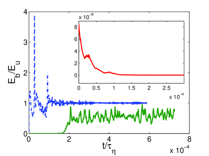
Figure 1: (Color online) Representative plots of the dynamo order parameter $E_{b}/E_{u}$ versus time $t/\tau_{\eta}$, with $\tau_{\eta}$ the magnetic-diffusion time, in the dynamo region (blue, dashed curve), near the dynamo boundary (green, full line), and in the no-dynamo regime (red, full line in the inset).

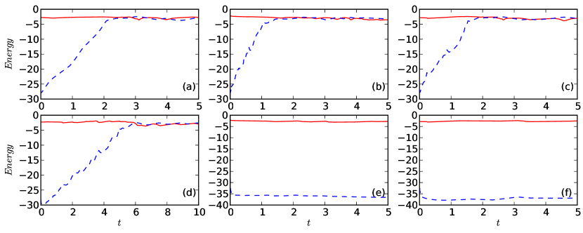
Figure 2: (Color online) Semi-log (base 10) plots of the kinetic (red full curve) and magnetic (blue dashed curve) energies versus time for (a) $Pr_{\rm M}=10^{2}$, (b) $Pr_{\rm M}=1$, (c) $Pr_{\rm M}=10^{-1}$, (d) $Pr_{\rm M}=10^{-2}$, (e) $Pr_{\rm M}=10^{-3}$, (f) $Pr_{\rm M}=10^{-6}$. The values of $\nu$ are (a) $10^{-5}$, (b) $10^{-5}$, (c) $10^{-6}$, (d) $10^{-7}$, (e) $10^{-4}$, and (f) $10^{-7}$; and the magnetic-diffusion time $\tau_{\eta}=\ell_{\rm 0}^{2}/\eta\simeq 2.52\times 10^{10},~{}2.52\times 10^{8},~{}2.52\times 10^{8},~{}2.52\times 10^{4}$ and $2.52\times 10^{4}$, respectively. Dynamo action occurs in (a)-(d) but not in (e) and (f).

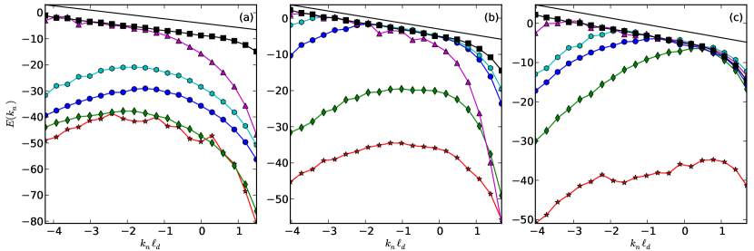
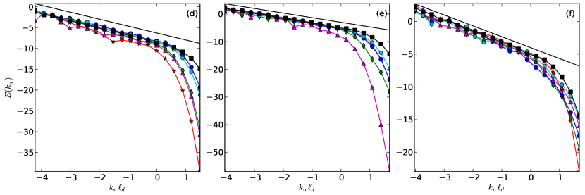
Figure 3: (Color online) Log-log (base 10) plots showing the time evolution of the magnetic-energy spectrum $E_{b}(k_{n})$ for representative parameter values at which dynamo action occurs: (a) $Pr_{\rm M}=10^{-2},\,\nu=10^{-7}$; (b) $Pr_{\rm M}=1,\,\nu=10^{-5}$, (c) $Pr_{\rm M}=10^{2},\,\nu=10^{-5}$; analogous plots for kinetic-energy spectra are shown in (d), (e), and (f), respectively. The curves with red stars, green diamonds, blue hexagons, cyan circles, and magenta triangles, are obtained, respectively, at $t=1,~{}5,~{}10,~{}15,$ and $100$; the dissipation scale $\ell_{d}\simeq 7.422\times 10^{-4}$ in (b), (c), (e), and (f); $\ell_{d}\simeq 4.779\times 10^{-4}$ in (a) and (d). Curves with black squares indicate velocity spectra before the seed magnetic field is introduced; the full black line shows a $k^{-5/3}$ spectrum for comparison.

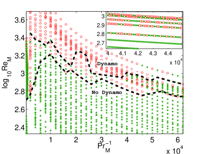
Figure 4: (Color online) The dynamo stability diagram in the $(Pr^{-1}_{\rm M},Re_{\rm M})$ plane: red circles indicate dynamo action; green stars are used if no dynamo occurs. The boundary between the two regions shows an intricate, interleaved pattern of fine, dynamo and no-dynamo regimes (see inset for a detailed view). We have drawn two black, dashed lines; the region above the upper one of these lines is predominantly in the dynamo regime; the area below the lower one of these lines is principally in the no-dynamo regime.

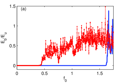
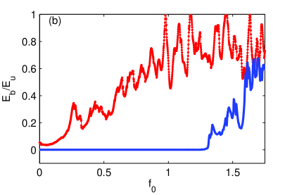
Figure 5: (Color online) Plots of the dynamo order parameter $E_{b}/E_{u}$ versus the forcing amplitude $f_{0}$ illustrating hysteretic behavior as $f_{0}$ is cycled across the dynamo boundary; here $Pr_{\rm M}=10^{-4}$ and $\nu=10^{-5}$. As $f_{0}$ increases, $E_{b}/E_{u}$ follows the blue, full line; if we now decrease $f_{0}$, then $E_{b}/E_{u}$ follows the red dotted line, and not the blue one, i.e., we have a hysteresis loop. We increase $f_{0}$ in steps of $1.0\times 10^{-3}$ from an initial value of $1.0\times 10^{-3}$; we keep $f_{0}$ constant for a time duration $10$ in (a) and $1$ in (b); the red, dotted-line segments of the hysteresis loops are obtained by decreasing $f_{0}$ at the same rates as for the blue, full-line segments.

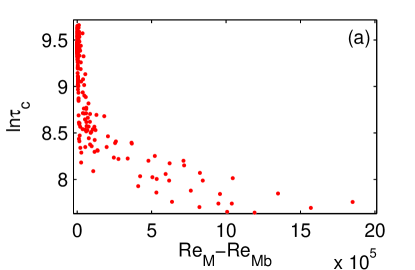
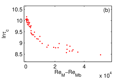
Figure 6: (Color online) Representative plots of $\ln\tau_{c}$ versus $Re_{\rm M}-Re_{\rm Mb}$ for parameter values at which dynamo action occurs; here $\tau_{c}$ is in units of the time step $\delta t$ and $Re_{\rm Mb}$ is the estimated position of the dynamo boundary: (a) $Pr_{\rm M}=1$ and (b) $Pr_{\rm M}=5\times 10^{-4}$. Note that the time $\tau_{c}$ required for dynamo action increases rapidly as we approach the dynamo boundary (the plot here is motivated by Eq. (27) in Ref. oxtoby ).

Given the numerical scheme that we have described in the previous Section, we obtain the time series for $u_{n}$ and $b_{n}$ from the MHD-shell-model equations. An analysis of these time series shows two types of nonequilibrium statistical steady states (NESS). We refer to the first as the no-dynamo state and to the second as the dynamo state. These states have been found in several earlier studies such as Refs. schekochihin ; ponty ; frisch ; chou ; minnini ; brandenburgdns ; plunian . Our main goal is to explore in detail the phase boundary between these two states. This can be done most easily by the introduction of a dynamo order parameter a natural candidate for which is the ratio $E_{b}/E_{u}$, where the fluid and magnetic energies are, respectively, $E_{u}=\frac{1}{2}\sum_{n}|u_{n}|^{2}$ and $E_{b}=\frac{1}{2}\sum_{n}|b_{n}|^{2}$. Representative plots of this order parameter are given as functions of time $t$ in Fig. 1: The blue, dashed curve shows the evolution of $E_{b}/E_{u}$ in the dynamo regime; note that here the dynamo order parameter rises rapidly, fluctuates significantly for $t/\tau_{\eta}\lesssim 2\times 10^{-4}$, and finally reaches a statistical steady state with equipartition, i.e., $E_{b}/E_{u}\simeq 1$. The red, full curve in the inset of Fig. 1 shows how $E_{b}/E_{u}$ vanishes rapidly in the no-dynamo state. The behavior of the dynamo order parameter is more complicated than these two simple possibilities in the vicinity of the phase boundary between dynamo and no-dynamo states as shown by the green, full curve in Fig. 1; $E_{b}/E_{u}$ rises much more slowly from zero than in the dynamo regime and then it fluctuates significantly for a long time; the difficulty of pinpointing the dynamo boundary is a consequence of these fluctuations.

The time series for the dynamo order parameter are obtained from those for $E_{u}$ and $E_{b}$; representative plots for these are shown, via red and blue-dashed curves, in Figs. 2(a), (b), (c), (d), (e), and (f) for a very large range of magnetic Prandtl numbers, namely, $Pr_{\rm M}=10^{2},~{}1,~{}10^{-1},~{}10^{-2},~{}10^{-3},$ and $10^{-6}$, respectively. The values of $\nu$ are (a) $10^{-5}$, (b) $10^{-5}$, (c) $10^{-6}$, (d) $10^{-7}$, (e) $10^{-4}$, and (f) $10^{-7}$; and the corresponding values of the diffusion time scale $\tau_{\eta}=\ell_{\rm 0}^{2}/\eta\simeq 2.52\times 10^{10},~{}2.52\times 10^{8},~{}2.52\times 10^{8},~{}2.52\times 10^{4}$ and $2.52\times 10^{4}$, respectively. Clearly dynamo action occurs in Figs. 2(a)-(d) but not Figs. 2(e) and (f). By obtaining many such plots we can identify the dynamo boundary in the $(Pr^{-1}_{\rm M},Re_{\rm M})$ plane as we discuss later.

In the dynamo regime the shell-model kinetic and magnetic energy spectra defined, respectively, by $E_{u}(k_{n})\equiv|u_{n}|^{2}/k_{n}$ and $E_{b}(k_{n})\equiv|b_{n}|^{2}/k_{n}$ evolve as shown in Fig. 3. In particular, in Figs. 3(a), (b), and (c) for $Pr_{\rm M}=10^{-2},~{}1,$ and $10^{2}$, respectively, we show the evolution of $E_{b}(k_{n})$ with time: the curves with red stars, green diamonds, blue hexagons, cyan circles, and magenta triangles, are obtained, respectively, for $t=1,~{}5,~{}10,~{}15,$ and $100$; the analogs of these plots for $E_{u}(k_{n})$ are given in Figs. 3(d), (e), and (f). Note that the initial growth of $E_{b}(k_{n})$ occurs principally at large values of $k_{n}$ if $Pr_{\rm M}$ is large, i.e., we have a small-scale dynamo; this growth of $E_{b}(k_{n})$ moves to low values of $k_{n}$ as $Pr_{\rm M}$ decreases; earlier studies chou ; plunian have observed similar trends but not over the large range of $Pr_{\rm M}$ we cover. As $E_{b}(k_{n})$ grows, the velocity spectra are also affected but much less than their magnetic counterparts as can be seen by comparing Figs. 3(d), (e), and (f) with Figs. 3(a), (b), and (c), respectively. In all these plots the curves with black squares indicate $E_{u}(k_{n})$ from the initial steady state for the GOY shell model; and the black lines with no symbols show the K41 $k_{n}^{-5/3}$ spectrum for comparison. From this line we see that the NESS that is obtained, once dynamo action has occurred, is such that both velocity and magnetic-field energy spectra display a substantial inertial range with K41 scaling; these inertial ranges are not large enough, at least near the dynamo boundary in our runs, for a reliable estimation of multiscaling corrections to the $-5/3$ exponent. If $Pr_{\rm M}\simeq 1$ then the scaling ranges in velocity and magnetic-field spectra are comparable; as $Pr_{\rm M}$ decreases (increases), the scaling range for the magnetic spectrum decreases (increases) relative to its counterpart in the velocity spectrum; these trends are clearly visible in the representative plots in Fig. 3.

We return now to the identification of the dynamo boundary. A close scrutiny of the plots in Fig. 2 shows that the initial growth of $E_{b}$ is not monotonic. It is important, therefore, to set a threshold value of the magnetic energy $E_{b}^{c}$: For a given pair of values for $Pr_{\rm M}$ and $Re_{\rm M}$, if $E_{b}(t)>E_{b}^{c}$ for $t>\tau_{c}$, where $\tau_{c}$ is the time at which the threshold value is crossed, we conclude that dynamo action occurs; if not, then there is no dynamo formation. By examining the growth of $E_{b}(t)$ we can, therefore, map out the dynamo boundary in the $(Pr^{-1}_{\rm M},Re_{\rm M})$ plane. The crossing time $\tau_{c}$ depends on $Pr_{\rm M}$ and $Re_{\rm M}$. Note that, if $\tau_{c}(Pr_{\rm M},Re_{\rm M})>t_{\rm max}$, the length of time for which we integrate Eqs.(3) and (4), we would conclude, incorrectly, that no dynamo action occurs for this of values of $Pr_{\rm M}$ and $Re_{\rm M}$. In other words the dynamo boundary depends on $t_{\rm max}$; we have checked this explicitly in several cases.

An important questions arises now: Is there a well-defined dynamo boundary in the $(Pr^{-1}_{\rm M},Re_{\rm M})$ plane as $t_{\rm max}\rightarrow\infty$? Earlier studies schekochihin ; ponty ; minnini have began to answer this question. They find that, if $t_{\rm max}\simeq\tau_{\eta}$, then a well-defined dynamo boundary is obtained. However, since they work with the MHD equations the error bars on this boundary are large and the range of values of $Pr_{\rm M}$ and $Re_{\rm M}$ rather limited.

The simplicity of our model allows us to carry out a systematic study of the dynamo boundary. We find that, at least in our shell model for MHD, we can obtain an asymptotic dynamo boundary (see Fig. 4) if we choose $E_{b}^{c}=0.9E_{u}$, i.e., we conclude that dynamo action has occurred if $E_{b}(t)$ exceeds $0.9E_{u}$; furthermore, if $E_{b}(t)$ falls below $10^{-35}$ we say that dynamo action will never be achieved. We continue the temporal evolution of Eqs.(3) and (4) till one of these criteria is satisfied. For all values of $Pr_{\rm M}$ and $Re_{\rm M}$ that we have used we find that this $t_{\rm max}$, the run time required to decide whether or not dynamo action occurs, is several orders of magnitude lower than $\tau_{\eta}$. We have also checked for several representative pairs of values for $Pr_{\rm M}$ and $Re_{\rm M}$ that runs of length $t_{\rm max}\simeq\tau_{\eta}$ do not change our conclusions about such dynamo action.

The dynamo boundary that we obtain is shown in the stability diagram of Fig. 4. Red circles indicate parameter values at which we obtain dynamo action whereas green stars are used for values at which no dynamo occurs. The most important result that follows from this stability diagram is that the boundary between dynamo and no-dynamo regimes is very complicated. It seems to be of fractal-type, with an intricate pattern of fine, dynamo regions interleaved with no-dynamo regimes. This is especially apparent in the inset of Fig. 4, which shows a detailed view of the stability diagram in the vicinity of the dynamo boundary. Earlier studies seem to have missed this fractal-type of boundary because they have not been able to examine the transition in as much detail as we have for our shell model. However, fractal-type boundaries between different dynamical regimes have been suggested in other extended dynamical systems; recent examples include the transition to turbulence in pipe flow bruno and different forms of spiral-wave dynamics in mathematical models for cardiac tissue shajahan . In Fig. 4 we have drawn two black, dashed lines; the region above the upper one of these lines is predominantly in the dynamo regime; the area below the lower one of these lines is predominantly in the no-dynamo regime. These two lines give an approximate indication of the error bars we might expect in the determination of the dynamo boundary in a study that cannot scan through points in the $(Pr_{\rm M}^{-1},Re_{\rm M})$ plane as finely as we have.

From Fig. 1 we see that the order parameter $E_{b}/E_{u}$ jumps from a very small value in the no dynamo region to a value $\simeq 1$ in the dynamo state. It is natural, therefore, to think of the dynamo boundary as a nonequilibrium, first-order boundary. In an equilibrium, first-order transition the order parameter shows hysteretic behavior if we scan through a first-order boundary by, say, changing, at a finite rate, the field that is conjugate to the order parameter mrao . It is natural to ask if we see such hysteretic behavior at the dynamo boundary. Indeed, we do, as we show in Fig. 5 where we cross the dynamo boundary by changing the amplitude $f_{0}$ of the forcing term in Eq.(3). Figure 5 shows representative plots of the dynamo order parameter $E_{b}/E_{u}$ versus $f_{0}$; these illustrate the hysteretic behavior that occurs when $f_{0}$ is cycled at a finite, nonzero rate across the dynamo boundary; here $Pr_{\rm M}=10^{-4}$ and $\nu=10^{-5}$. As $f_{0}$ increases, $E_{b}/E_{u}$ follows the blue, full line: it increases and then saturates; fluctuations are superimposed on these mean trends. If we now decrease $f_{0}$, then $E_{b}/E_{u}$ follows the red dotted line, and not the blue one, i.e., we have a hysteresis loop. The faster the rate at which we change $f_{0}$ the wider is the hysteresis loop as is known from studies of hysteresis in spin systems mrao . Here we increase $f_{0}$ in steps of $1.0\times 10^{-3}$ from an initial value of $1.0\times 10^{-3}$; we keep $f_{0}$ constant for a time period $10$ in Fig. 5(a) and $1$ in Fig. 5(b); the red, dotted-line segments of the hysteresis loops are obtained by decreasing $f_{0}$ at the same rates as for the blue, full-line segments; the loop in the former case is narrower than in the latter.

Given the analogy with first-order transitions that we have outlined above, it is natural to ask if nucleation-type phenomena oxtoby are also associated with dynamo formation. It would be interesting to check this in a DNS of the MHD equations. At the level of our shell model, the best we can do is to try to see if, for a given $Pr_{\rm M}$, when we obtain a dynamo, the time required for dynamo action $\tau_{c}$ diverges as we approach the dynamo boundary. Our data are consistent with an increase of $\tau_{c}$ as we approach this boundary from the dynamo side as shown by the representative plots in Fig. 6. However, it is hard to fit a precise form to the behavior of $\tau_{c}$ near the dynamo boundary partly because of the complicated nature of this boundary which makes it difficult to estimate the position $Re_{\rm Mb}$ reliably (the plot in Fig. 6 is motivated by the form of Eq. (27) in Ref. oxtoby ).

IV Conclusions

We have presented a detailed study of dynamo action in a shell model of turbulence basu ; frick ; brandenburgshell . Our study has been designed to explore the nature of the boundary between dynamo and no-dynamo regimes in the $(Pr^{-1}_{\rm M},Re_{\rm M})$ plane over a much wider range of $Pr_{\rm M}$ than has been attempted in earlier numerical studies. The dynamo boundary emerges as a first-order nonequilibrium phase boundary between one turbulent, nonequilibrium statistical steady state (NESS) and another footnote . This point of view is implicit in earlier work, e.g., in studies of the Kazantsev dynamo kazantsev or in studies that view dynamo generation as a subcritical bifurcation busse77 ; pontyetal07 ; kuangetal08 . One of these studies pontyetal07 has remarked that when dynamo action “ … is obtained in a fully turbulent system, where fluctuations are of the same order of magnitude as the mean flow … the traditional concept of amplitude equation may be ill-defined and one may have to generalize the notion of “subcritical transition” for turbulent flows …”. We believe that the natural generalization is the nonequilibrium, first-order transition we suggest above. We have explored the explicit consequences of such a view in far greater detail than has been attempted hitherto. In particular, the ratio $E_{b}/E_{u}$ is a convenient order parameter for this nonequilibrium phase transition; it shows hysteresis across the dynamo boundary like order parameters at any first-order transition; and nucleation-type phenomena also seem to be associated with dynamo formation. Last, and perhaps most interesting, we find that the dynamo boundary seems to have a fractal character; this provides a natural explanation for the large error bars in earlier attempts to determine this boundary schekochihin ; ponty ; plunian . Furthermore, this fractal-type boundary might well be the root cause of magnetic-field reversals discussed, e.g., in Refs. benzi ; pintonreversal .

It is important to check, of course, that our shell-model results carry over to the MHD equations. This requires large-scale DNS that might well be beyond present-day computing capabilities if we want to explore issues like the possible fractal nature of the dynamo boundary. However, analogs of the hysteretic behavior we mention above have been obtained in DNS studies of the MHD equations busse77 ; pontyetal07 ; kuangetal08 ; hysteresis has also been seen in a numerical simulation that includes turbulent convection sim+bus09 . In some of these studies hysteretic behavior is obtained by changing the viscosity of the magnetic Prandtl number. We have obtained hysteresis by changing the forcing; this change of forcing might be easier to effect in experiments than a change of the viscosity or magnetic diffusivity.

To the best of our knowledge, earlier studies have not noted the increase in the dynamo-formation time $\tau_{c}$ as the dynamo boundary is approached from the dynamo side. We have suggested that this is akin to the increase in the time required to form a critical nucleus as we approach a first-order boundary oxtoby . It would be interesting to see if such an increase of $\tau_{c}$ can be obtained in DNS studies of dynamo formation with the MHD equations. It is worth noting here that some DNS studies ponty have suggested that simulation times comparable to the diffusion time scale $\tau_{\eta}$ are required to confirm dynamo formation; by contrast our shell-model study yields dynamo action on a much shorter time $\tau_{c}$, which increases as we approach the dynamo boundary. Perhaps the large simulation times required for dynamo action in full MHD simulation might have arisen because these simulations have been carried out in the vicinity of the dynamo boundary.

To settle completely whether the dynamo boundary is of fractal-type, very long simulations might be required to make sure that the apparent fractal nature is not an artifact of long-lived metastable states. To make sure that our calculations do not suffer from such an artifact, we have carried out very long runs for representative points in the region of the dynamo boundary in Fig. 4; we have found that these long runs do not change our results. Furthermore, it is useful to check whether, instead of one dynamo boundary, there is a sequence of transitions, with more and more complicated temporal behaviors for the order parameter, as has been seen in the turbulence-induced melting of a nonequilibrium vortex crystal crystalmelt . We have not found any conclusive evidence for this but, in the vicinity of the dynamo boundary, the order parameter can oscillate for fairly long times (see, e.g., the green full curve in Fig. 1). To decide conclusively whether these oscillations characterize a new nonequilibrium oscillating state, different from the simple dynamo and no-dynamo NESSs we have mentioned, requires extensive numerical studies that lie beyond the scope of this paper.

In equilibrium statistical mechanics different ensembles are equivalent; in particular, we may determine a first-order phase boundary by using either the canonical or the grand-canonical ensemble. However, such an equivalence of ensembles does not apply to transitions between different nonequilibrium statistical steady states (NESSs); examples may be found in driven diffusive systems acharyya or in the turbulence-induced melting of a nonequilibrium vortex crystal crystalmelt . Given that the dynamo boundary separates two turbulent NESSs, we might expect that this boundary might depend on precisely how the system is forced. Evidence for this exists already: For example, the dynamo boundary depends on whether a stochastic external force is used schekochihin or whether a Taylor-Green force is used ponty ; furthermore, this boundary is different if the fluid is helical brandenburgdns , as in most astrophysical dynamos.

We hope our study of dynamo formation in a shell model for MHD will stimulate both DNS and experimental studies designed to explore the first-order nature of the dynamo transition.

- (1) A. R. Choudhuri, The Physics of Fluids and Plasmas: An Introduction for Astrophysicists (Cambridge University Press, Cambridge, UK, 1998).
- (2) G. Rüdiger and R. Hollerbach, The Magnetic Universe: Geophysical and Astrophysical Dynamo Theory (Wieley, Weinheim, 2004).
- (3) H. Goedbloed and S. Poedts, Principles of Magnetohydrodynamics With Applications to Laboratory and Astrophysical Plasmas (Cambridge University Press, Cambridge, UK, 2004).
- (4) D. Biskamp, Magnetohydrodynamic Turbulence (Cambridge University Press, Cambridge, UK, 2003).
- (5) M.K. Verma, Phys. Rep. 401, 229 (2004).
- (6) Focus on Magnetohydrodynamics and the Dynamo Problem, New J. Phys. 9, (2007).
- (7) A.A. Schekochihin et al., New J. Phys. 4, 84 (2002); Phys. Rev. Lett. 92, 054502 (2004); New J. Phys. 9, 300 (2007); A.A. Schekochihin, S.C. Cowley, and S.F. Taylor, Astrophys. J. 612, 276 (2004).
- (8) P. H. Roberts and G. A. Glatzmaier, Rev. Mod. Phys. 72, 1081 (2000).
- (9) F. Pétrélis and S. Fauve, Europhys. Lett. 22, 273 (2001); 76, 602 (2006); S. Fauve and F. Pétrélis, in Peyresq Lectures on Nonlinear Phenomena, edited by J.-A. Sepulchre (World Scientific, Singapore, 2003), Vol. 2, pp. 1–64; S. Fauve, F. Pétrélis, C.R. Physique 8, 87 (2007).
- (10) A. Gailitis et al., Phys. Rev. Lett. 84, 4365 (2000); Phys. Rev. Lett. 86, 3024 (2001); Rev. Mod. Phys. 74, 973 (2002); Surv. Geophys. 24, 247 (2003); Phys. Plasmas 11, 2838 (2004).
- (11) R. Stieglitz and U. Müller, Phys. Fluids 13, 561 (2001); U. Müller, R. Stieglitz, and S. Horanyi, J. Fluid Mech. 498, 31 (2004); U. Müller and R. Stieglitz, Nonlin. Proc. Geophys. 9, 165 (2002).
- (12) N.L. Peffley, A.B. Cawthorne, and D.P. Lathrop, Phys. Rev. E 61, 1063 (2000); W.L. Shew and D.P. Lathrop, Phys. Earth Planet. Inter. 153, 136 (2005).
- (13) M. Bourgoin et al., Phys. Fluids 14, 3046 (2002); 16, 2529 (2004); L. Marié et al., Magnetohydrodynamics 38, 163 (2002); R. Monchaux et al., Phys. Rev. Lett. 98, 044502 (2007).
- (14) A. Kolmogorov, Dokl. Akad. Nauk. SSSR, 31, 538 (1941); Proc. R. Soc. London, Ser. A 434, 15 (1991).
- (15) S. Boldyrev and F. Cattaneo, Phys. Rev. Lett. 92, 144501 (2004).
- (16) Y. Ponty, H. Politano, and J.-F. Pinton, Phys. Rev. Lett. 92, 144503 (2004); Y. Ponty et al., Phys. Rev. Lett. 94, 164502 (2005); New J. Phys. 9, 296 (2007).
- (17) S. Kenjere and K. Hanjalić, Phys. Rev. Lett. 98, 104501 (2007); New J. Phys. 9, 306 (2007).
- (18) M. Meneguzzi, U. Frisch, and A. Pouquet, Phys. Rev. Lett. 47, 1060 (1981); J. Léorat, A. Pouquet, and U. Frisch, J. Fluid Mech. 104, 419 (1981).
- (19) H. Chou, Astrophys. J., 556, 1038 (2001).
- (20) P.D. Minnini, D.C. Montgomery, and A. Pouquet, Phys. Fluids 17, 035112 (2005); P.D. Mininni et al., Astrophys. J. 626, 853 (2005); P. Mininni, A. Alexakis, and A. Pouquet, Phys. Rev. E 72, 046302 (2005); P.D. Mininni and A. Pouquet, Phys. Rev. Lett. 99, 254502 (2007).
- (21) A. Brandenburg, Astrophys. J., 697, 1206(2009).
- (22) A.B. Iskakov et al., Phys. Rev. Lett. 98, 208501 (2007).
- (23) A. Basu, A. Sain, S. Dhar, and R. Pandit, Phys. Rev. Lett. 81, 2687 (1998); C. Kalelkar and R. Pandit, Phys. Rev. E 69, 046304 (2004).
- (24) P. Frick and D. Sokoloff, Phys. Rev. E 57, 4155 (1998); S.A. Lozhkin, D.D. Sokolov, and P.G. Frick, Astron. Rep. 43, 753 (1999).
- (25) A. Brandenburg, K. Enqvist, and P. Olesen, Phys. Rev. D 54, 1291 (1996).
- (26) P. Giuliani and V. Carbone, Europhys. Lett. 533(5), 527 (1998).
- (27) J. Leorat, P. Lallemand, J.L. Guermond, and F. Plunian, in Dynamo and Dynamics: A Mathematical Challenge, edited by P. Chossat et al. (Kluwer Academic, Dordrecht, 2001), p. 25-33; R. Stepanov and F. Plunian, J. Turbulence, 7, N 39 (2006).
- (28) M.K. Verma et al., Phys. Rev. E 78, 036409 (2008).
- (29) R. Benzi and J.-F. Pinton, eprint arXiv 0906.0427 (2009).
- (30) M. Rao, H.R. Krishnamurthy, and R. Pandit, J. Phys. Condens. Matter 1, 9061 (1989); Phys. Rev. B 42, 856 (1990).
- (31) Y. Ponty et al, Phys. Rev. Lett., 99, 224501 (2007).
- (32) T. Bohr, M.H. Jensen, G. Paladin, and A. Vulpiani, Dynamical Systems Approach to Turbulence (Cambridge University, Cambridge, UK, 1998).
- (33) E. Gledzer, Sov. Phys. Dokl. 18, 216 (1973); K. Ohkitani and M. Yamada, Prog. Theor. Phys. 81, 329 (1989);
- (34) P. Perlekar and R. Pandit, New J. Phys. 11, 073003 (2009).
- (35) T.M. Schneider, B. Eckhardt, and J.A. Yorke, Phys. Rev. Lett. 99, 034502 (2007).
- (36) T.K. Shajahan, S. Sinha, and R. Pandit, Phys. Rev. E 75, 011929 (2007); T.K. Shajahan, A.R. Nayak, and R. Pandit, PLoS ONE 4(3), e4738 (2009).
- (37) D.W. Oxtoby, J. Phys. Condens. Matter 4, 7627 (1992).
- (38) We use the expression first-order transition as in equilibrium statistical mechanics since the order parameter (the first derivative of a free energy) jumps at the transition. Since there is no free energy for the NESSs we consider, one can, just as well, refer to this as a discontinuos transition.
- (39) For example, see the following: A.P. Kazantsev, Soviet Phys.-JETP 26, 1031 (1968); D. Vincenzi, J. Stat. Phys. 106, 1073 (2002); A.A. Schekochihin et al. Phys. Rev. Lett. 92, 084504 (2004).
- (40) F.J. Busse., J. Geophys., 43, 441 (1977).
- (41) W. Kuang, W. Jiang, and T. Wang Geophys. Res. Lett., 35, L14204 (2008).
- (42) M. Bourgoin, R. Volk, N. Plihon, P. Augier and J.-F. Pinton, New J. Phys. 8, 329 (2006).
- (43) R.D. Simitev and F.H. Busse, Europhysics Lett. 85, 19001 (2009).
- (44) P. Perlekar and R. Pandit, submitted for publication, eprint arxiv 0910.3096.
- (45) M. Acharyya, A. Basu, R. Pandit and S. Ramaswamy, Phys. Rev. E 61, 1139 (2000).