Spatial pattern formation and polarization dynamics of a nonequilibrium spinor polariton condensate

Abstract

Quasiparticles in semiconductors — such as microcavity polaritons — can form condensates in which the steady-state density profile is set by the balance of pumping and decay. By taking account of the polarization degree of freedom for a polariton condensate, and considering the effects of an applied magnetic field, we theoretically discuss the interplay between polarization dynamics, and the spatial structure of the pumped decaying condensate. If spatial structure is neglected, this dynamics has attractors that are linearly polarized condensates (fixed points), and desynchronized solutions (limit cycles), with a range of bistability. Considering spatial fluctuations about the fixed point, the collective spin modes can either be diffusive, linearly dispersing, or gapped. Including spatial structure, interactions between the spin components can influence the dynamics of vortices; produce stable complexes of vortices and rarefaction pulses with both co- and counter-rotating polarizations; and increase the range of possible limit cycles for the polarization dynamics, with different attractors displaying different spatial structures.

I Introduction

The experimental realization of quantum condensation of quasiparticles with finite lifetimes has opened the possibility to study situations where the steady states of the condensate are not just controlled by energetics, but involve also consideration of pumping and decay, leading to steady states with quasiparticle currents. The exploration of the possible behavior exhibited in these systems is driven particularly by recent experimental progress in microcavity polaritonsKasprzak et al. (2006); Balili et al. (2007); Lagoudakis et al. (2008); Utsunomiya et al. (2008); Amo et al. (2009a, b) and magnonsDemokritov et al. (2006); Demidov et al. (2008); Chumak et al. (2009); Dzyapko et al. (2009) (as well as more exotic realizations in heliumVolovik (2008)). Microcavity polaritons are the quasiparticles that result from strong coupling between photons confined in planar semiconductor microcavities and excitons confined in quantum wells. The photons are confined by Bragg reflectors to a two-dimensional cavity, and for small in-plane momentum have an effectively quadratic dispersion, with a mass of the order of $10^{-5}$ – $10^{-4}$ of the free electron mass. From strong coupling between these photon states and exciton states in quantum wells, new normal modes arise: polaritons. These are hybrid light–matter particles, which have both a light effective mass, as well as sufficient interactions to allow a quasi-equilibrium particle distribution to be established. However, the distribution is only quasi-equilibrium, since the photon component is not perfectly confined, so polaritons have a finite lifetime, and to maintain a steady state population, continuous pumping is required. Even when the energy distribution of polaritons looks reasonably thermal, this does not mean effects of finite lifetime may be neglected, as one may have thermalized energy distributions on top of steady state flows driven by the pumping and decay.

Experimentally, it is observed that above a threshold pumping strength, an accumulation of low energy polaritons is accompanied by: a significant increase in temporal coherence, spatial coherence that extends over the entire cloud of polaritonsKasprzak et al. (2006); Balili et al. (2007), the appearance of quantized vorticesLagoudakis et al. (2008), suggestions of changes to the excitation spectrumUtsunomiya et al. (2008), and a robustness of polariton propagation to disorderAmo et al. (2009a, b). Of these, the observation of spontaneous vorticesLagoudakis et al. (2008) in polariton condensates provides a strong hint that the steady states of the system are affected by the flow of particles. For a more general introduction to microcavity polaritons, their condensation, and the physical systems studied there exist several reviews or books, e.g., Refs. Ciuti et al., 2003; Keeling et al., 2007; Kavokin et al., 2007.

The aim of this article is to investigate the rich varieties of behavior that come from combining spatial profiles driven by particle flow with the dynamics due to the spin degree of freedom that microcavity polaritons also possess. The effects of this spin degree of freedom have been previously considered in equilibrium: due to the weak attractive interaction between opposite spin polarizations, a condensate is expected to be linearly polarizedLaussy et al. (2006); Shelykh et al. (2006), i.e., to have an equal density of left- and right-circularly polarized components. Applying a magnetic field can then lead to a phase transition, as the density of one circular polarization increases, and the other decreases, leading through an elliptically polarized phase to a single circularly polarized condensateRubo et al. (2006); Keeling (2008). In the absence of further symmetry breaking, the linear or elliptically polarized phase has two gapless modes, corresponding to two broken symmetries: the overall polariton phase, and the direction of linear polarization (i.e., orientation of elliptical polarization). The transition to a circular polarized state is thus a phase transition, as such a phase has only a single broken symmetry, and a single gapless mode.

Assuming no other symmetry breaking terms, the linearly polarized condensate can have independent vortices of the left- and right-circularly polarized componentsRubo (2007); such polarization-dependent phase winding has recently been observedLagoudakis et al. (2009). These two vortices are not completely independent. Even in the absence of any further symmetry breaking, there is a short-range density-density interaction between vortices of opposite polarizationsRubo (2007); Keeling (2008), however such a term does not depend on the circulations of the two vortices. If one also takes account of TE-TM splitting of the electromagnetic modesPanzarini et al. (1999), this leads to a term that splits linear polarization states according to whether the polarization is parallel or perpendicular to the polariton momentum; as such, this provides a circulation dependent interaction between vortices of the two polarizationsToledo Solano and Rubo (2009). In addition, real materials are expected to possess a small splitting between linear polarization states due to asymmetry of the quantum-well interfaces in non-centro-symmetric crystalsAleiner and Ivchenko (1992); such a splitting can also be controlled by applying electrostatic fieldsMalpuech et al. (2006) or stressSnoke . Such terms will again induce interactions between vortices of the left- and right-circular polarization, and if strong enough, will lead to a pinning of the polarization of a polariton condensate, as has been observed in experiment Amo et al. (2005); Klopotowski et al. (2006); Kasprzak et al. (2006, 2007).

Considering the splitting of linear polarizations as a phase-locking term between the two circular polarization components, and combining this with a magnetic field that favors one or other circular polarization, one has a Josephson problemLeggett (2001), where the energy favoring linear polarization is a Josephson coupling, and the magnetic field leads to a bias between the two fields. Shelykh et al. (2008) have considered the interplay between these spinor Josephson oscillations, and Josephson coupling between two different spatial modes of a trapped polariton condensate, showing that complex behavior can arise in this four-mode system without pumping and decay. A similar problem has also been studied in the context of spinor condensates of cold atoms in double well potentialsSatija et al. (2009); Juliá-Díaz et al. (2009). If one does include pumping and decay then even the two-mode system (i.e., just the dynamics of the spin component) can show a rich variety of behavior Wouters (2008); Eastham (2008). Due to dissipation, the dynamics settles on an attractor, which may either correspond to a phase-locked (i.e., linearly polarized) state, or may correspond to a limit cycle, in which the phase difference between the two polarization components continually increases, with the cyclic nature arising from $2\pi$ periodicity in the phase difference. There also exist parameter ranges where there is bistability, so that which attractor the system settles on depends on the initial conditions. In this article, we will both review this two-mode dynamics, and then extend to the case of including many spatial modes in addition to the spin dynamics.

To describe multiple spatial modes in a trapped, pumped, decaying condensate, a mean-field approach to this problem leads to a complex Gross–Pitaevskii equationKeeling and Berloff (2008); Wouters et al. (2008). It is also possible to include fluctuations beyond mean-field theory within such a formalism by quantum stochastic approachesWouters and Savona (2009). As well as describing the spatial structure of nonequilibrium condensates, the complex Gross–Pitaevskii equation has also been applied in a wide range of areas, see for example Refs. Aranson and Kramer, 2002; Staliunas and Sanchez-Morcillo, 2003. One application which is very closely connected to microcavity polaritons is the dynamics of lasers propagating through strongly nonlinear materials, where combinations of cubic and quintic nonlinearities can produce a state with a preferred density, sometimes referred to as “liquid light”Michinel et al. (2002, 2006). The results in this article suggest that consideration of polarization dynamics in such materials may also provide interesting results.

By considering the spinor complex Gross–Pitaevskii equation to describe the spinor condensate in an harmonic trap, several new classes of attractors are seen to occur in addition to those present for the two-mode system. There are limit cycles describing small oscillations of the phase difference between the two components, and limit cycles with $4\pi$ periodicity of the phase difference. In addition, the different dynamical attractors correspond to different spatial profiles, in which the presence or absence of vortex lattices can be influenced by the applied magnetic fields.

As well as describing the steady state profiles, the complex Gross–Pitaevskii equation can describe the normal modes for small fluctuations about such steady states. In the absence of a spatial trap, one notable consequence of including pumping and decay is that the long-wavelength modes of a dissipative condensate are modified, to become diffusiveWouters and Carusotto (2007a); Szymańska et al. (2006, 2007); similar results are seen both for incoherent pumped condensates, and for optical parametric oscillation, where scattering of pumped polaritons into signal and idler states is modified by bosonic enhancement due to the population of the signalWouters and Carusotto (2006); Wouters and Carusotto (2007b). From this standpoint, another purpose of this article is to address how the combination of pumping, decay, and symmetry-breaking terms modify the spectrum of the spinor condensate. While a diffusive mode for the overall polariton density and phase always exists, the long-wavelength modes for spin modes can show a range of behaviors: diffusive, linearly dispersing, or gapped, dependent on the balance of decay and symmetry-breaking terms.

The remainder of this article is arranged as follows. In Section II we introduce the model of spinor condensates as a system of coupled Gross–Pitaevskii equations with pumping and decay terms. By neglecting the spatial variations of polarized components we discuss the bifurcation diagrams for a two-mode system in Section III. The normal modes of the homogeneous system are obtained in Section IV. In Section V we study the stability of cross-polarized vortices. The detailed study of the dynamics of the full trapped system is performed in Section VI. In Section VII we discuss how various regimes can be detected in experiments. The conclusions in Section VIII summarize our findings.

II Model for spinor polaritons

The model we consider in this article consists of the complex Gross-Pitaevksii equation (cGPE) as described in Ref. Keeling and Berloff, 2008, taking into account the two possible polarizations of polaritons, written in the basis of left- and right-circular polarized states, denoted by $\psi_{L,R}$. In addition to the terms discussed in Ref. Keeling and Berloff, 2008, three new parameters arise from considering the spin degree of freedom in an applied magnetic field. Firstly, in addition to an interaction with the total polariton density $H_{U_{0}}=(U_{0}/2)(|\psi_{L}|^{2}+|\psi_{R}|^{2})^{2}$, there is an attractive interaction between opposite spin species, $H_{U_{1}}=-2U_{1}|\psi_{L}|^{2}|\psi_{R}|^{2}$. Secondly, there is a magnetic field term $H_{\Omega_{B}}=(\Omega_{B}/2)(|\psi_{L}|^{2}-|\psi_{R}|^{2})$, and finally there is a symmetry breaking term $H_{J_{1}}=J_{1}(\psi_{L}\psi_{R}^{\dagger}+\text{H.c.})$, which may naturally ariseKasprzak et al. (2006, 2007) due to asymmetry at the quantum-well interfacesAleiner and Ivchenko (1992), or may be induced by electric fieldsMalpuech et al. (2006) or stressSnoke . Put together, these yield the coupled cGPE:

$$i\partial_{t}\psi_{L}=\left[-\frac{\hbar^{2}\nabla^{2}}{2m}+V(r)+U_{0}|\psi_{L}|^{2}+(U_{0}-2U_{1})|\psi_{R}|^{2}\right.\\ \left.+\frac{\Omega_{B}}{2}+i\left(\gamma_{\text{eff}}-\kappa-\Gamma|\psi_{L}|^{2}\right)\right]\psi_{L}+J_{1}\psi_{R},$$ (1)

with the analogous equation for $\psi_{R}$ following by replacing $\psi_{L}\leftrightarrow\psi_{R}$ and $\Omega_{B}\to-\Omega_{B}$. In this article, we will either neglect $V(r)$ (in sections III, IV), or consider a harmonic trap, $V(r)=m\omega_{0}^{2}r^{2}/2$. In either case, we will rescale energies and lengths in terms of the harmonic-oscillator energy $\hbar\omega_{0}$, and length $l$ such that $\hbar\omega_{0}=\hbar^{2}/2ml^{2}$. By additionally rescaling the density such that $U|\psi|^{2}\to\hbar\omega_{0}|\psi|^{2}$ the cGPE can be written as:

$$i\partial_{t}\psi_{L}=\bigg{[}-\nabla^{2}+v(r)+|\psi_{L}|^{2}+(1-u_{a})|\psi_{R}|^{2}+\frac{\Delta}{2}\\ +i\left(\alpha-\sigma|\psi_{L}|^{2}\right)\bigg{]}\psi_{L}+J\psi_{R}$$ (2)

with the definitions $\alpha=(\gamma_{\text{eff}}-\kappa)/\hbar\omega_{0},\sigma=\Gamma/U_{0},J=J_{1}/\hbar\omega_{0},\Delta=\Omega_{B}/\hbar\omega_{0},u_{a}=2U_{1}/U_{0}$. If considering a harmonic trap, then $v(r)=V(lr)/\hbar\omega_{0}=r^{2}$, otherwise we will take $v(r)=0$.

The dimensionless parameter $u_{a}$ describes the extent of spin anisotropy of the interaction; using the estimate in Ref. Renucci et al., 2005 we take $u_{a}=1.1$. From estimates of the polarization splitting in Refs. Klopotowski et al., 2006; Kasprzak et al., 2007, we take $J_{1}\simeq 0.1\text{--}0.2\text{meV}$. Using the estimates of trap frequency given in Ref. Keeling and Berloff, 2008, we will take $0\leq\alpha\leq 10,\sigma=0.3$, and we may write the dimensionless splitting $J\simeq 1$; in the numerical results, we will consider a variety of values of $J$ around this value.

The spatially extended, harmonically trapped system is unstable unless pumping is restricted to a finite spotKeeling and Berloff (2008). For our studies of this system, we therefore consider a circular pumping spot with a cutoff radius $r_{0}$: $\alpha\rightarrow\alpha\Theta(r_{0}-r)$. For constant pumping strength, $r_{0}$ determines whether the system forms vortices spontaneouslyKeeling and Berloff (2008).

III Review of the two-mode model

In order to provide a basis from which to understand the behavior observed in the trapped system, it is first useful to review the results that occur in the “two-mode model”, where spatial variation of each component is neglected, so the coupled complex Gross–Pitaevskii equation reduces to two equations for the variables $\psi_{L},\psi_{R}$. This model was studied by Wouters (2008), where the conditions for the existence of a steady state (i.e., synchronized) solution were found. As $\Delta$ increased, Wouters (2008) found that a synchronized solution could persist for some range of $\Delta$, with an increasing phase and density difference between the two modes, until at some critical $\Delta$ the steady state vanished. Near the critical $\Delta$, the existence of bistability was noted. This section will both summarize these previous results, as well as analyze the behavior of the desynchronized solution, showing that the dynamics is analogous to that of the damped driven pendulum, or current-biased Josephson junctionStrogatz (1994).

To discuss the dynamics, it is convenient to reparametrize using:

$$\psi_{L,R}=\sqrt{\rho_{L,R}}e^{i(\phi\pm\theta/2)},\quad R=\frac{\rho_{L}+\rho_{R}}{2},\quad z=\frac{\rho_{L}-\rho_{R}}{2},$$

and write coupled equations for $\theta,R,z$. (The global phase $\phi$ does not affect the dynamics.) In visualizing the dynamics, one may consider a Bloch vector, defined by $x=\sqrt{\rho_{L}\rho_{R}}\cos(\theta),y=\sqrt{\rho_{L}\rho_{R}}\sin(\theta),z$, in terms of the above variables. Since there is pumping and decay, the length of the Bloch vector is not conserved, hence there is a dynamical equation for $R=\sqrt{x^{2}+y^{2}+z^{2}}$. The coupled equations have the form:

$$\dot{\theta} =-\Delta-2u_{a}z+\frac{2Jz\cos(\theta)}{\sqrt{R^{2}-z^{2}}}$$ (3)

$$\dot{z} =2(\alpha-2\sigma R)z-2J\sqrt{R^{2}-z^{2}}\sin(\theta)$$ (4)

$$\dot{R} =2\sigma\left(\frac{\alpha}{\sigma}R-R^{2}-z^{2}\right).$$ (5)

Writing the equations in this form firstly allows one to understand the basic effects of pumping and decay on the dynamics, and, secondly, will be shown below to reduce to the damped driven pendulum in a relevant limit.

For a steady state, it is clear that the condition $\dot{R}=0$ defines a Bloch surface, $R(z)$. One may then study the dynamics of points that start on this surface to characterize the nature of the transition as $\Delta$ increases. As shown in Fig. 1, each starting point $z,\theta$ is attracted either to a fixed point, or to a limit cycle. The fixed point is the synchronized solution; the limit cycle is the desynchronized solution, in which the phase difference $\theta$ between the two spin components is changing — this behavior is a cycle since the dynamics are periodic under $\theta\to\theta+2\pi$. As $\Delta$ increases, there is a lower critical $\Delta_{c,\text{lower}}$ below which the all initial conditions on the Bloch surface flow to the synchronized solution, and an upper critical $\Delta_{c,\text{upper}}$ which corresponds to the previously foundWouters (2008) point beyond which synchronized solutions can no longer exist.

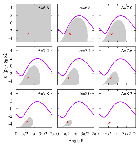
Figure 1: (Color online) Basin of attraction of fixed point and limit cycle for full two-mode Josephson problem. Each panel is for a given value of $\Delta$, as indicated, and shows a colormap according to the final state found by starting from the given initial conditions $\theta,z$. Points that flow to the fixed point are colored gray, others are white. The fixed point is marked by a red cross, and the limit cycle (when it exists) by the magenta line.

The behavior seen in Fig. 1 can be understood by noticing that the choice of parameters used puts one in the “Josephson regime” of the Josephson equationsLeggett (2001), i.e., $u_{a}R\gg J$, and that in addition the typical dynamics obey $z\ll R$. In this case, Eq. (5) simply reduces to $R=\alpha/\sigma$. Then, by eliminating $z$ from Eq. (3,4), one finds:

$$\ddot{\theta}+2\alpha\dot{\theta}=-2\alpha\Delta+4u_{a}J\frac{\alpha}{\sigma}\sin(\theta).$$ (6)

This equation describes a damped driven pendulum, or alternatively a current-biased Josephson junction. (N.B., due to our choice of sign of $J$, “gravity” for the pendulum acts to drive $\theta\to\pi$). The behavior of Eq. (6) is well known (see, e.g., Ref. Strogatz, 1994); for large damping $\alpha$ there is a simple transition at $\Delta_{c,\text{upper}}=2u_{A}J/\sigma$ between fixed points for $\Delta<\Delta_{c,\text{upper}}$ and limit cycles above. For smaller damping (explicitly, for for $\alpha<0.595\sqrt{4u_{a}J\alpha/\sigma}$), there is a range of bistability, where both limit cycles and fixed points may be foundUrabe (1955). The inset of Fig. 2 shows the bifurcation diagram determined from Eq. (3–5), and for comparison, the value $\Delta_{c,\text{upper}}$ and the critical damping that result from the approximations leading to Eq. (6).

As well as explaining the classes of behavior seen, Eq. (6) may be used to explain the critical behavior near $\Delta_{c,\text{lower}}$. For $\alpha$ sufficiently small that bistability exists, then near $\Delta_{c,\text{lower}}$, the period of the limit cycle grows like $T\propto|\ln[\Delta-\Delta_{c,\text{lower}}]|$. In the context of the current problem, this period relates to the average chemical potential difference between the two components, $\langle\dot{\theta}\rangle=\langle\mu_{L}-\mu_{R}\rangle=2\pi/T$. For large $\Delta$, one eventually reaches $\mu_{L}-\mu_{R}=\Delta$. The evolution of $\langle\mu_{L}-\mu_{R}\rangle$ is illustrated in Fig. 2, which plots the spectral weight $|\tilde{\psi}_{L}(\omega)|^{2}$, choosing initial conditions so the limit cycle is obtained for all $\Delta>\Delta_{c,\text{lower}}$.

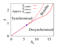
Figure 2: (Color online) Fourier transform of $\psi_{L}(t)$, showing bifurcation of frequencies as $\Delta$ is increased, and illustrating critical behavior $\omega\sim 1/\ln|\Delta-\Delta_{c}|$. Initial conditions for each $\Delta$ are chosen so that a limit cycle (i.e., desynchronized solution) is found for all $\Delta>\Delta_{c,\text{lower}}$. Inset: Regions of stability of the synchronized and desynchronized solutions found from Eq. (3–5). The dotted line marks the approximate $\Delta_{c,\text{upper}}$ appropriate in the Josephson regime, Eq. (6), and the $\ast$ marks the known bifurcation pointUrabe (1955) in that regime.

IV Normal modes in the extended homogeneous system

Before considering the interplay of spin dynamics with the spatial profile of a trapped condensate, one may first consider a simpler problem involving the interplay of spin and spatial dynamics — the finite momentum normal modes of the pumped, decaying spinor condensate. The normal modes of the spinor condensate without pumping and decay were discussed in Rubo et al. (2006); Keeling (2008). In the equilibrium case, for small $|\Delta|$, there is an elliptical condensate (i.e., a finite density of both spin components) and there are two gapless linear modes, describing excitations of the global phase, and the relative phase of the two components. When $|\Delta|$ becomes large enough to cause a transition to a circularly polarized state, only a single gapless mode survives, describing phase modes of the condensed component. On the other hand, the presence of pumping and decay is known to replace the linear dispersion of the phase modes with a diffusive behavior at small momentumSzymańska et al. (2006, 2007); Wouters and Carusotto (2007b, a). The aim of this section is to see how these two effects are combined. The result is that while the global phase mode remains diffusive, the real part of the relative phase mode can be either gapped, linearly dispersing, or diffusive according to the value of $\Delta$ chosen. In the following, we will first present numerical results for the normal-mode frequencies, and then discuss how these can be straightforwardly interpreted in the same Josephson regime as discussed above.

For the purpose of numerically calculating the normal modes, it is simplest to consider the Bogoliubov parametrization of fluctuations at some wavevector $k$ (allowing for decay) as:

$$\psi_{L,R}(t,r)=e^{-i\mu t}\psi^{0}_{L,R}+\\ e^{-i\mu t}\left(u_{L,R}e^{-i\omega t-\kappa t-i\mathbf{k}\cdot\mathbf{r}}+v_{L,R}^{\ast}e^{i\omega t-\kappa t+i\mathbf{k}\cdot\mathbf{r}}\right).$$ (7)

Substituting this into Eq. (2), and linearizing in $u,v$ yields the secular equation $\mathrm{Det}[(\omega-i\kappa)\mathbbm{1}-M]=0$, where in the basis $\chi=(u_{L},v_{L},u_{R},v_{R})^{T}$, the matrix $M$ is

$$M=\left(\begin{array}[]{cccc}A_{L}&B_{L}&C_{L}&D_{L}\\ -B_{L}^{\ast}&-A_{L}^{\ast}&-D_{L}^{\ast}&-C_{L}^{\ast}\\ A_{R}&B_{R}&C_{R}&D_{R}\\ -B_{R}^{\ast}&-A_{R}^{\ast}&-D_{R}^{\ast}&-C_{R}^{\ast}\end{array}\right).$$ (8)

Noting that for plane waves, the kinetic energy term $-\nabla^{2}\to k^{2}$, the matrix elements are:

$$A_{L} =k^{2}-J\frac{\psi_{R}^{0}}{\psi_{L}^{0}}+(1-i\sigma)|\psi_{L}^{0}|^{2}, B_{L} =(1-i\sigma)(\psi^{0}_{L})^{2}$$

$$C_{L} =J+(1-u_{a})\psi^{0}_{L}\psi_{R}^{0\ast}, D_{L} =(1-u_{a})\psi^{0}_{L}\psi^{0}_{R},$$

and similarly with $L\leftrightarrow R$. The normal modes calculated this way are shown in Figs. 3, 4. Figure 3 shows the modes at $k=0$ (lower panels) as well as the value of $\Delta$, and the densities $\rho_{L,R}$ (upper panels) corresponding to a solution with a given value of $\theta$. [This is to make use of the fact that the steady state of Eqs. (3–5) can be found explicitly for $\Delta,\rho_{L,R}$ as a function of $\theta$ (see Ref. Wouters, 2008).]

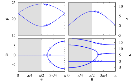
Figure 3: (Color online) Steady states, and damping of uniform fluctuations. All panels are plotted as a function of the phase difference, $\theta$, between the two circular polarization components. Top left: densities of components in steady state solution. Top right: Detuning corresponding to given solution. Bottom: Real (left) and imaginary (right) parts of frequency for small fluctuations about the steady state. The gray shaded region is unstable to small fluctuations. The crosses mark the conditions used for the finite $k$ spectra in Fig. 3. Plotted for $\alpha=6.5,\sigma=0.3,J=1.0,u_{a}=1.1$.

In Fig. 3, the range of $\theta$ is restricted to $[0,\pi]$, since the range $[\pi,2\pi]$ is equivalent to this, after swapping $L\leftrightarrow R$ and $\Delta\to-\Delta$. Within this range, only values $\theta>\theta_{c}\simeq\pi/2$ correspond to stable solutions. As only the modes at $k=0$ are shown, there is always a zero mode corresponding to global phase rotations. The other three modes divide into an overdamped mode (largest imaginary part), and a pair of modes which can be either overdamped or underdamped, as seen by the bifurcation of the real part at $\theta=1.964$. Three values of $\theta$ (corresponding to three different applied detunings $\Delta$) are chosen to illustrate the overdamped, critically damped, and underdamped cases, and the normal modes with finite $k$ are shown for these points in Fig. 4. In the overdamped case (for $\theta$ near $\pi/2$), both the relative-phase and global-phase modes are diffusive at small $k$. When underdamped, the relative-phase mode always has a nonzero real frequency. When critically damped, the real part of the relative-phase mode has a linear dispersion. We will next discuss how this behavior can be understood in the Josephson regime.

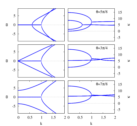
Figure 4: (Color online) Spectra of normal modes in a uniform system; showing real (left) and imaginary (right) parts of each mode separately. The three rows correspond to the three points marked by crosses in Fig. 3. In all cases the total density modes are diffusive, while the spin mode changes from diffusive (top row, $\theta$ nearest $\pi/2$), to linearly dispersive (middle row) to underdamped spin oscillations (bottom row, $\theta$ nearest $\pi$).

To understand the modes qualitatively, it is clearest to work in the basis of $R,z,\theta,\phi$. Extending Eqs. (3–5) to include spatial gradients via a Madelung transformation, one finds the equations:

$$\dot{R} =-\nabla\left(2R\nabla\phi+z\nabla\theta\right)+2\alpha R-2\sigma(R^{2}+z^{2})$$ (9)

$$\dot{z} =-\nabla\left(2z\nabla\phi+R\nabla\theta\right)+2(\alpha-2\sigma R)z$$

$$\qquad-2J\sqrt{R^{2}-z^{2}}\sin\theta$$ (10)

$$\dot{\phi} =\frac{X_{L}+X_{R}}{2}-(2-u_{a})R-\frac{JR}{\sqrt{R^{2}-z^{2}}}\cos(\theta)$$ (11)

$$\dot{\theta} =(X_{L}-X_{R})-2u_{a}z-\frac{2Jz}{\sqrt{R^{2}-z^{2}}}\cos(\theta)-\Delta,$$ (12)

where we have introduced the shorthand $X_{L,R}=(\nabla^{2}\sqrt{\rho_{L,R}})/\sqrt{\rho_{L,R}}-(\nabla\theta_{L,R})^{2}$, with $\theta_{L,R}=\phi\pm\theta/2$. When considering fluctuations about the uniform state, the gradient terms simplify, as expressions such as $(\nabla\theta)^{2}$ are necessarily second order in the fluctuations, and so may be neglected. We will make the same approximations as led to Eq. (6) (i.e., assume $J\ll u_{a}R,z\ll R$), and use the steady-state solution in this limit ($R=\alpha/\sigma,J\sin(\theta)=-\sigma z$) to simplify the equations for fluctuations. If one writes the fluctuations as $\chi=(\delta R,\delta z,\delta\phi,\delta\theta)^{T}$ then since these are real variables, the normal modes have the time dependence $\chi(t)=\chi\exp(-i\omega t-\kappa t)$, giving a secular equation:

$$\mathrm{Det}\left[(i\omega+\kappa)\mathbbm{1}+M_{0}+k^{2}M_{1}+\mathcal{O}(k^{4})\right]=0,$$ (13)

where $M_{n}$ indicates an expansion in powers of momentum, to understand the small $k$ dispersion. The first two terms are:

$$M_{0} =\left(\begin{array}[]{cccc}-2\alpha&0&0&0\\ -2\sigma z&-2\alpha&0&-2JR\cos(\theta)\\ -2+u_{a}&0&0&0\\ 0&-2u_{a}&0&0\end{array}\right)$$ (18)

$$M_{1} =\left(\begin{array}[]{cccc}0&0&2R&z\\ 0&0&2z&R\\ -1/2R&z/2R^{2}&0&0\\ z/R^{2}&-1/R&0&0\end{array}\right)$$ (23)

The nature of the $k=0$ normal modes is immediately clear: $\phi$ has no restoring force, and so has a zero frequency oscillation; $R$ has a damping rate $2\alpha$, and so describes a decaying mode; $z$ and $\theta$ are mixed, and have modes with frequencies given by:

$$(i\omega+\kappa)(i\omega+\kappa-2\alpha)-4u_{a}JR\cos(\theta)=0.$$ (24)

Noting that $\cos(\theta)$ is negative, and that the prefactor is the same as that of $\sin(\theta)$ in Eq. (6), one may write:

$$-4u_{a}JR\cos(\theta)=\Omega_{p}^{2},$$ (25)

where $\Omega_{p}(\theta)$ is a “plasma frequency” describing the restoring force as a function of angle. The normal modes are $\omega-i\kappa=-i\alpha\pm\sqrt{\Omega_{p}^{2}-\alpha^{2}}$. The transition between under- and overdamping occurs because for $\theta\simeq\pi$ the restoring force is large so $\Omega_{p}>\alpha$, while as $\theta\to\theta_{c}\simeq\pi/2$, the restoring force vanishes, and so there is an intermediate value of $\theta$ (and hence $\Delta$) at which $\Omega_{p}=\alpha$, describing the critical damping. Note that whatever the choice of parameters, an overdamped regime will always exist since $\Omega_{p}$ must always tend to zero at $\theta_{c}$. However if $\alpha$ is sufficiently large the underdamped regime may vanish. The approximate expressions for the eigenvalues $\omega-i\kappa=0,-i\alpha\pm\sqrt{\Omega_{p}(\theta)^{2}-\alpha^{2}},-2i\alpha$ match the general form seen in the bottom panel of Fig. 3, it is apparent that the full problem has some additional variation of damping rate with $\theta$, not captured by the approximations used in the above expressions.

One may now explain the linear dispersion at this critical damping as arising from degenerate perturbation theory, allowing a $k^{2}$ perturbation to give a $\propto k$ splitting. Setting $\Omega_{p}=\alpha$, and writing $\omega-i\kappa=-i\alpha+\eta$, then expanding Eq. (13) to leading order in $\eta,k$ gives:

$$0=\eta^{2}-k^{2}\left[\frac{\alpha^{2}}{2u_{a}R}+2u_{a}R\right],$$ (26)

hence describing modes $\omega-i\kappa=-i\alpha+c_{\text{eff}}k$. Note that although these modes have a linear dispersion of the real part as a function of $k$, they have a lifetime that remains finite as $k\to 0$. As such, this may provide an example where linear dispersion of a given mode in a condensed system need not imply superfluidity of the associated density. Further work is required to determine the current-current response function in this system, which will determine whether there is a difference of transverse and longitudinal response for spin currents, however superfluidity of the spin current is not expected here, since the spin orientation is locked by the Josephson term $J$. The linear dispersion arises only when the damping matches frequency of this phase-locking term, producing critical damping.

V Stability of cross-polarized vortices with pumping and decay

When an harmonic trap is introduced, the existence of steady state currents can destabilize the Thomas–Fermi like density profile, and lead to spontaneous rotating vortex latticesKeeling and Berloff (2008). Before addressing how this instability interacts with the polarization degree of freedom, we first discuss the simpler question of the dynamics and stability of individual vortices of opposite polarization. One should note first that a single vortex in a pumped decaying condensate already has a more complicated structure than the vortex without pumping and decay — the vortex becomes a spiral vortex, with both radial and azimuthal currents; see appendix A for further discussion.

Considering a spinor condensate system with vortices in both polarization components, there is an interplay between the weak attractive coupling that invites the vortices to have their cores aligned irrespective of their circulation, the Josephson coupling that discourages the alignment of vortices of opposite circulation and the detuning that stabilizes such alignment. To illustrate these possibilities we consider several examples. The notation $(\pm n,\pm m)$ refers to condensates with vortices of topological charge $\pm n$ ($\pm m$) in left (right) condensate. From Eq. (2), with $v(r)=r^{2}$, the following set of stability scenarios are found:

$J=0$:

All $(\pm 1,0)$ and $(\pm 1,\pm 1)$ vortex complexes are dynamically stable.

$J\neq 0,\Delta=0$:

Solutions $(+1,+1)$ are stable, $(\pm 1,0)$ and $(+1,-1)$ are unstable. Depending on the strength of $J$, vortices may start precessing around the center of the trap, move beyond the boundary forming either a pair of rarefaction waves with opposite velocities or a complex $(+1,+1)$, or disappear at the condensate’s edge and bringing in two aligned pairs of vortices $(+1,+1)$ and $(-1,-1)$. Fig. 5 illustrates these possibilities for $\alpha=4.4,r_{0}=3,\sigma=0.3$ and $J=0.5,1,1.5,2$.

$J\neq 0,\Delta\neq 0$:

For a given $J$, any sufficiently large $\Delta$ allows the vortex complexes $(+1,-1)$ and $(\pm 1,0)$ to stabilize. Fig. 6 shows such stabilized $(+1,-1)$ complex for $J=1,\Delta=8.$

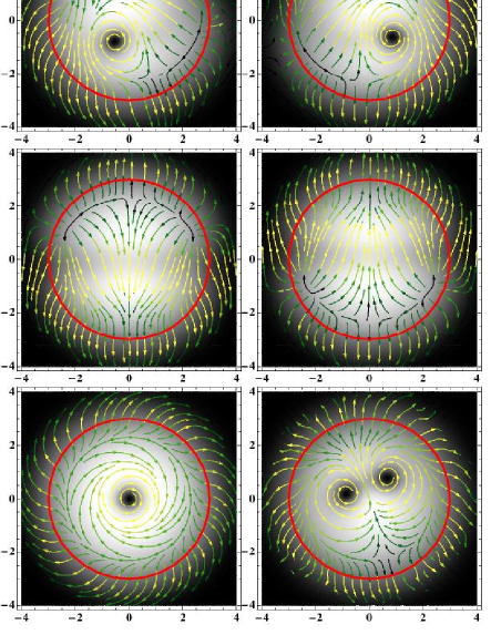
Figure 5: (Color online) The outcome of instability of the vortex state $(+1,-1)$ for $\alpha=4.4,\sigma=0.3,r_{0}=3,\Delta=0,$ and $J=0.5$ (top row), $J=1$ (second row), $J=1.5$ (left bottom) and $J=2$ (right bottom). The initial state is $\psi_{\pm}=\sqrt{\Theta(\mu_{\text{TF}}-r^{2})}(x\pm{\rm i}y)/\sqrt{r^{2}+1/(\mu_{\text{TF}}\delta)}$ where $\psi_{R}=\psi_{-},\psi_{L}=\psi_{+}$, $\mu_{\text{TF}}=3\alpha/2\sigma$ and $\delta$ is the vortex core parameter; see Appendix A. Depicted are the density plots and streamlines of $\psi_{L}$ (left panels in first and second row, bottom row) and $\psi_{R}$ (right panels in first and second row). Luminosity is proportional to the magnitude of the density for density plots and to the velocity for streamlines. The size of the pumping is shown as a circle of radius $r_{0}=3$. For $J=0.5$ the final state consists of two precessing vortices of opposite circulation. For $J=1$ the system evolves into a pair of two gray solitons. For $J=1.5$ the vortex of the negative circulation in $\psi_{R}$ leaves and a vortex of positive circulation enters the cloud. For $J=2$ both vortices leave the condensate and two pairs of vortices of opposite circulation enter. For $J=1.5$ and $J=2$ $\psi_{L}=\psi_{R}$, so only $\psi_{L}$ is shown.

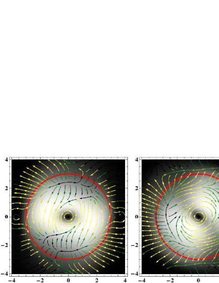
Figure 6: (Color online) Stable state of cross-polarized vortices $(+1,-1)$ for $\alpha=4.4,\sigma=0.3,r_{0}=3,\Delta=8,$ and $J=1$. Depicted are the density plots and streamlines of $\psi_{L}$ (left) and $\psi_{R}$ (right). Luminosity is proportional to the magnitude of the density for density plots, and velocity is shown by streamlines. The size of the pumping is shown as a circle of radius $r_{0}=3$.

The stationary state shown in Fig. 5 for $J=1$ is the vorticity-free, but not radially symmetric, solution of Eq. (2). These are analogous to the rarefaction solitary waves of the nonlinear Schrödinger equation discovered by Jones and Roberts Jones and Roberts (1982). In trapped 2D condensates these waves were also found Mason and Berloff (2008): they form as two vortices of opposite circulation disappear at the boundary of the condensate. In the conservative GPE these waves propagate with velocities exceeding the velocity of any vortex pair. In spinor damped/driven condensates two such solutions induce flow in opposite directions forming a stationary complex. The plots of the real and imaginary parts of $\psi_{L}$ and $\psi_{R}$ shown in the left panel of Fig. 7, and the density plots of Fig. 5 can be compared to the bottom panel of Fig. 9 and the left panel of Fig. 10 of Ref. Mason and Berloff, 2008. It also follows from simulations that $\psi_{L}(x,y)=\psi_{R}(x,-y)$, so the found stationary state satisfies a one component Ginzburg–Landau equation

$$i\partial_{t}\psi = [-\nabla^{2}+r^{2}+|\psi|^{2}\psi$$ (27)

$$+{\rm i}(\alpha\Theta(r_{0}-r)-\sigma|\psi|^{2})]\psi+J\psi(x,-y).$$

This also suggests a way to generate solitary waves in spinor condensates. The dark soliton (obtained by phase imprinting, for instance) will undergo a transverse snake instability and form two stationary pairs of vortices of opposite circulation, whereas starting with a $(+1,-1)$ complex one will obtain stationary rarefaction pulses.

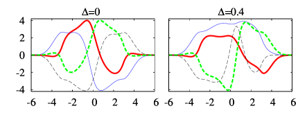
Figure 7: (Color online) Real (thick lines) and imaginary (thin lines) parts of $\psi_{L}$ (solid lines) and $\psi_{R}$ (dashed lines) of the rarefaction wave complex as a stationary solution of Eq. (2) with $v(r)=r^{2}$ for $\alpha=4.4,\sigma=0.3,J=1$ and $\Delta=0$ (left) and $\Delta=0.4$ (right) plotted along the axis of density symmetry. The functions are antisymmetric with respect to the origin $\psi_{L}(0,-y)=\psi_{R}(0,y)$ for $\Delta=0$, but not for $\Delta\neq 0$.

As $\Delta$ increases, the rarefaction waves in two components lose their antisymmetry and the density minima move away from the center as the right panel of Fig. 7 illustrates. For intermediate $\Delta$, complexes combining a rarefaction wave in one component with a precessing vortex in the other component emerge; for even larger $\Delta$ two vortices of opposite circulation move around in the condensate. Finally, for even larger $\Delta$, their cores overlap and vortices move to the center of the condensate. These possibilities are illustrated on Figs. 6 and 8. The cross-polarized vortices deform the condensate to a slightly oblate form as seen in the density plots of Fig. 6. The streamlines and the density plots indicate that the vortices coexist with rarefaction waves that rotate in the counterclockwise direction.

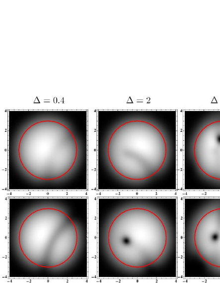
Figure 8: (Color online) Density plots $|\psi_{L}|^{2}$ (top row) and $|\psi_{R}|^{2}$ (bottom row) for the outcome of instability of cross-polarized vortices obtained by numerical integration of Eq. 2 with $v(r)=r^{2}$, $\alpha=4.4,\sigma=0.3,J=1$ and various $\Delta$. The initial state is the same as in Fig. 5. Luminosity is proportional to density. The size of the pumping is shown as a circle of radius $r_{0}=3$. For $\Delta=0.4$ two rarefaction pulses form a stationary complex. For $\Delta=2$ a vortex of negative circulation in the $R$ component is coupled to a rarefaction pulse in the $L$ component. For $\Delta=4$ the two vortices of opposite circulation do not align their cores. For $\Delta=2$ and $\Delta=4$ the complexes precess around the center with the individual vortices moving along an epitrochoid; see also Fig. 9.

The vortex trajectories with pumping, decay and a spin degree of freedom are nontrivial. For a one-component conservative GPE, a single vortex moves perpendicularly to the background density gradient due to the Magnus forceRubinstein and Pismen (1994); Kivshar et al. (1998) (the speed of the motion is however nonuniversal, and depends on the global condensate shape Mason and Berloff (2008)). For a two-component conservative GPE with vortices in both components, there is an additional advection of each vortex by the flow pattern of the other component. Including also pumping and decay, the trajectories of the vortices are yet more complicated, as illustrated in Fig. 9 for a $(+1,-1)$ complex with $J=1,\Delta=4$. Both vortices move along trajectories closely resembling epitrochoids, and the distance between the vortices varies quasi-periodically with time. Similarly complicated cycloid trajectories of vortices are known for two-layer fluids with one vortex in each layer — such behavior has been seen for example in models of tropical vorticesKhandekar and Rao (1975).

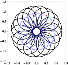
Figure 9: (Color online) Trajectories of vortices in the complex $(+1,-1)$ obtained by numerical integration of Eq. 2 with $v(r)=r^{2}$, $\alpha=4.4,\sigma=0.3,J=1$ and $\Delta=4$, and with pumping in a radius $r_{0}=3$. These parameters are the same as for the density profiles in the right hand column of Fig. 8. The trajectory of the vortex of positive (negative) circulation in the left (right) component is shown as thick black (thin blue) line. The start (end) points of the time interval plotted are shown as red (green) filled circles. Note that the vortex trajectories are not closed.

VI The trapped system

We study the time-dependent problem defined by Eq. (2) with a harmonic trapping potential $v(r)=r^{2}$ by numerical integration, using a fourth-order, finite-difference approximation in space and a fourth-order Runge–Kutta method in time. Pumping is restricted to a circular spot of radius $r_{0}$ centered at the bottom of the trap, as described at the end of section II. In all of the following, we take the experimentally realistic parametersKeeling and Berloff (2008); Kasprzak et al. (2006); Richard et al. (2005) $\alpha=4.4$ and $\sigma=0.3$. With this choice of parameters, the critical radius can be estimated from the Thomas–Fermi approximation for the problem without polarizationKeeling and Berloff (2008) as $r_{0_{c}}\simeq 4.7$. This section will present and discuss the transition between synchronized and desynchronized states, and the interplay with the instability to vortex lattice formation. Section VI.1 first addresses the value of $\Delta$ for which a transition occurs, as one changes the size of the pumping spot, and coupling $J$. Section VI.2 will then discuss in greater detail the nature of the new attractors near the critical $\Delta$ that occur when one includes spatial degrees of freedom.

VI.1 Critical $\Delta$, bistability and internal Josephson effect

Let us start with the simplest trapped problem, taking $J=1.0$ and $r_{0}=3.0$. We study the behavior of the system as the detuning $\Delta$ is increased in the following way: starting at $\Delta=0$ from a Gaussian initial state, we let the system evolve until a steady solution is reached. We then increase $\Delta$ in steps, taking for each new $\Delta$ the final state at the previous $\Delta$ as the new initial state. For each value of $\Delta$, the chemical potentials of the two polarization components are calculated (see appendix C for details). The result is shown in the left panel of Fig. 10. The components stay synchronized, sharing a common chemical potential, up to $\Delta\simeq 7.0$. As the detuning is increased further, the components desynchronize and AC Josephson oscillations occur between them (Fig. 11). Note that as the components desynchronize, the chemical potentials show an oscillatory time dependence. Fig. 10 shows a time average in this case.

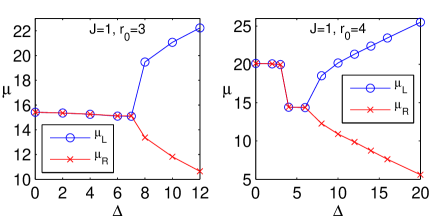
Figure 10: (Color online) Chemical potentials of the two polarization components plotted against stepwise increased detuning $\Delta$. For solutions with time-dependent chemical potentials, a time average is shown.

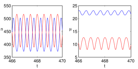
Figure 11: (Color online) Josephson oscillations in the desynchronized solution at $\Delta=12.0,r_{0}=3.0,J=1.0$ in the limit of large time. Left: $n=\int|\psi|^{2}\,d^{2}r$ as a function of time. Right: The chemical potentials of the two polarization components. (Time given in units of $2/\omega_{0}$. Blue and red color denote $L$ and $R$ components, respectively.)

In terms of a suitably defined, spatially averaged phase difference $\theta$ between the components (see appendix C), the desynchronization transition corresponds to a transition from a fixed point to a limit cycle in the $(\theta,\dot{\theta})$ plane, in direct analogy to the two-mode problem (see Fig. 12 and compare with Fig. 1).

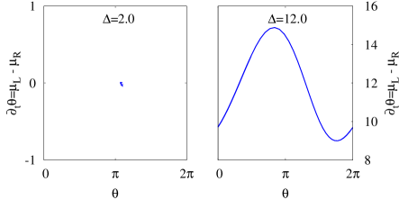
Figure 12: (Color online) Phase portraits for the trapped problem with $J=1.0$ and $r_{0}=3.0$. Left: synchronized solution for small detuning. Right: desynchronized solution in the limit of large detuning (corrected for numerical precession).

The right panel of Fig. 10 shows the chemical potentials of the two polarization components as the detuning is increased stepwise in a system pumped in a spot with radius $r_{0}=4.0$. The progression from the synchronized solution at small detunings to the desynchronized solution in the limit of large detunings is now more complicated than for a small pumping spot. $r_{0}=4.0$ is too small a pumping radius for vortices to form spontaneously in the corresponding one-component systemKeeling and Berloff (2008). Accordingly, the spinor system with zero detuning develops circularly symmetric densities, identical in both components (but with different phases for the two components). For small enough detunings, the system stays synchronized, the densities adjusting to accommodate the common, constant chemical potential (left-most panels of Fig. 13).

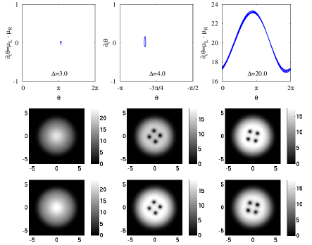
Figure 13: (Color online) Progression from fully synchronized solution via formation of vortex lattice to fully desynchronized solution at $r_{0}=4.0$ and $J=1.0$. Top: phase portraits for the phase difference $\theta$ (a numerical precession has been removed from the $\Delta=20.0$ plot). Middle and bottom: total densities of the $L$ and $R$ components, respectively.

As the detuning increases beyond $\Delta\simeq 3.0$ the rotational instability of the high-angular-momentum modes Keeling and Berloff (2008) reappears, and a four-vortex lattice forms in both components. At this point, the smaller component is sufficiently depressed by the detuning that the effective critical radius is smaller than the pumping radius. The suppressed component becomes rotationally unstable and drags the larger component along. This transition to a vortex-lattice solution causes the (common) chemical potential to drop, as shown in Fig. 10.

While the two components remain on average phase locked, the drop in chemical potential at the formation of the vortex lattice is accompanied by a time-dependence of the chemical potentials, which oscillate together around a common mean. Due to the amplitude of the oscillations being slightly larger in the larger component, the fixed point in the $(\theta,\dot{\theta})$ plane turns into a small limit cycle, but with only small variations of $\theta$ unlike the $2\pi$ periodic cycles in the desynchronized phase. (Middle panels of Fig. 13.)

Finally, as $\Delta$ becomes large, the components desynchronize completely. This situation is shown in the right-hand panels of Fig. 13. The difference in space-averaged phase now traces out a limit cycle winding through the full $2\pi$.

The overall progression from synchronized solutions at small $\Delta$ to desynchronized solutions with Josephson oscillations holds very generally for different values of the Josephson coupling $J$ and also for both small (no vortices) and large (vortex lattice) pumping-spot sizes. The mechanism in both cases is the same: the synchronized solution is upheld by adjusting the densities and a steady interconversion current forms. After desynchronization, the densities revert to profiles as for the single component condensate, with the average density set by the balance of pumping and decay, but with an additional time-dependent interconversion current. Fig. 14 shows density profiles of typical synchronized solutions with and without vortices, and also a snapshot of a desynchronized solution.

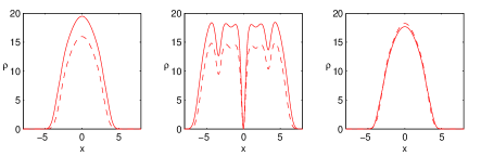
Figure 14: (Color online) Density profiles along the $x$-axis for representative examples of synchronized and desynchronized solutions. Left: synchronized solution without vortices ($r_{0}=3.0,\Delta=4.0$). Middle: synchronized solution with vortex lattice ($r_{0}=6.0,\Delta=4.0$). Right: desynchronized solution without vortices ($r_{0}=3.0,\Delta=12.0$). Dashed and solid lines indicate left and right-polarized components, respectively. $J=1.0$ for all three examples.

We also performed calculations where we reset the initial conditions to a Gaussian density profile, with equal phase of the two polarization components for each value of $\Delta$. Based on the results of the two-mode model shown in Fig. 1, such initial conditions would be expected to find the limit cycle whenever it exists, whereas the stepwise increase of $\Delta$ discussed above is intended to follow the fixed point. In these calculations with resetting of initial conditions, desynchronized solutions generally develop at smaller $\Delta$, as one should expect if there is a region of coexistence of synchronized and desynchronized solutions. Fig. 15 shows the highest $\Delta$ yielding synchronized solutions for different $r_{0}$ and different $J$, both for stepwise increased $\Delta$ (top left) and calculation directly from Gaussian initial conditions (top right). Comparing the two plots gives an estimate of the region of coexistence. An example ($J=1.0,r_{0}=3.0$) showing the region of bistability is given in the bottom left panel. Note that the difference between stepwise increased $\Delta$ and reset to Gaussian initial condition for each $\Delta$ vanishes for large detunings. This need not be the case for larger $r_{0}$ or larger $J$, where more than one desynchronized, meta-stable state (distinguished by numbers of vortices) may be possible at high $\Delta$.

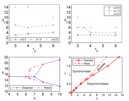
Figure 15: (Color online) Top: Highest $\Delta$ yielding synchronized solutions plotted as a function of $r_{0}$ for $J=0.5,1.0$ and $2.0$. Left: $\Delta$ increased stepwise. Right: resetting initial conditions for each $\Delta$. Bottom left: bifurcation of chemical potentials (plotted as in Fig. 10) for the two approaches, indicating the region of bistability for the example $J=1.0,r_{0}=3.0$. Bottom right: sketch of regions of stability of synchronized and desynchronized solutions for $r_{0}=3.0$. Compare with inset of Fig. 2.

Our calculations suggest that the spatially extended system allows for a rich variation of behaviors. Notably, interconversion due to the Josephson coupling between the components need not be uniform in space. The interconversion rate is easily calculated from the time-dependent local phase difference $\theta(\mathbf{r})=\phi_{R}(\mathbf{r})-\phi_{L}(\mathbf{r})$ as

$$\left.\frac{\partial\rho_{L}(\mathbf{r})}{\partial t}\right|_{J}=-\left.\frac{\partial\rho_{R}(\mathbf{r})}{\partial t}\right|_{J}=2J\sqrt{\rho_{L}(\mathbf{r})\rho_{R}(\mathbf{r})}\sin\left(\theta(\mathbf{r})\right),$$ (28)

familiar from the Josephson effect as found in any textbookTilley and Tilley (1990); Leggett (2001). Note that Eq. (4) describes the same physics for the two-mode model. Fig. 16 shows a map of the interconversion rate $\left.\partial_{t}\rho_{1}\right|_{J}$ at two close points in time in the large-time limit of the solution directly from Gaussian initial conditions with $J=1.0,r_{0}=6.0,\Delta=16.0$. This solution is desynchronized and exhibits Josephson oscillations. However, at any given time there is interconversion in both directions at different points in space.

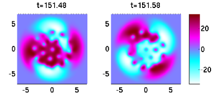
Figure 16: (Color online) Spatially nonuniform interconversion rate $\left.\partial_{t}\rho_{1}\right|_{J}$ at two different, but close, times. $J=1.0,r_{0}=6.0,\Delta=16.0$.

Calculations directly from Gaussian initial conditions at large detuning with a large pumping spot ($r_{0}=6.0$) indicate that solutions are possible in which the polarization components develop counter-rotating vortex lattices. This leads to rapid density modulations, particularly around the edge of the cloud, and a corresponding pattern of interconversion in opposite directions. In this case, the Josephson oscillations are suppressed and the total (scaled) mass $n=\int|\psi|^{2}\,d^{2}r$ exhibits rapid, small-amplitude oscillations. These effects are shown in Fig. 17.

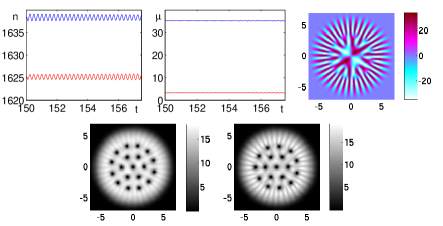
Figure 17: (Color online) Top from left to right: scaled mass $n=\int|\psi|^{2}\,d^{2}r$, chemical potentials and interconversion rate $\left.\partial_{t}\rho_{1}\right|_{J}$ for a desynchronized solution with counter-rotating components. Bottom: densities of the $L$ and $R$ polarization components, respectively. (Note that the gray scale has been adjusted for each component separately to accentuate the density modulations.) $J=1.0,r_{0}=6.0,\Delta=32.0$.

VI.2 Phase portraits of more complicated attractors

The spatial degree of freedom allows a number of behaviors of the $(\theta,\dot{\theta})$ phase portrait that are not possible in the two-mode problem, which only allows fixed points (synchronized solutions) and limit cycles with winding number $1$ (desynchronized solutions). In the spatially extended system, these behaviors are exemplified in Fig. 12 for a system without vortices. Both these two classes of attractor can also be seen when a vortex lattice exists. In addition, the spatial degree of freedom gives rise to several new classes.

We have already noted in Fig. 13 an example of a synchronized limit cycle. This can be distinguished from the desynchronized limit cycle by the winding number, $\int\dot{\theta}dt/2\pi$, over one period. The synchronized limit cycle has winding number $0$, and the desynchronized cycles have winding number $1$. We also find an example of limit cycle with winding number $2$, shown in Fig. 18. This solution also exhibits another behavior not possible in the two-mode model: a retrograde loop. This solution appears in calculation directly from a Gaussian initial condition at $\Delta=6.4$, which is barely above $\Delta_{c}$ for $J=1.0,r_{0}=3.0$. For larger $\Delta$ the loop quickly becomes a cusp and then disappears.

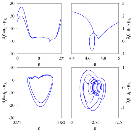
Figure 18: (Color online) Top: Limit cycle with winding number $2$ and retrograde loop. Left panel shows a blow-up of the loop. A numerical precession has been removed from these plots. ($J=1.0,r_{0}=3.0,\Delta=6.4$.) Bottom left: Possibly quasi-periodic behavior similar to a limit cycle with winding number $0$ ($J=2.0,r_{0}=3.0,\Delta=14.0$ from stepwise increase). Bottom right: Possible chaotic attractor ($J=2.0,r_{0}=3.0,\Delta=10.0$ from stepwise increase).

The bottom panels of Fig. 18 show two other behaviors found when stepwise increasing the detuning in a system with a strong Josephson coupling ($J=2.0$). Both these solutions are basically synchronized (the time average of the chemical potential is the same for both components). However, the large detuning causes the chemical potentials to differ at most instances in time, resulting in behaviors similar to the limit cycles with winding number $0$, but which appear to have a chaotic attractor and/or quasi-periodic behavior.

VII Experimental signatures

To directly observe rotating vortex lattices in experiments would require time-resolved measurements on timescales of the order of the trap frequency, which would be challenging with current experimental configurations. It is however possible to see signatures of a vortex lattice in the momentum- and energy-resolved photoluminescence spectrum, which can be directly measured in the far field. The spectral weight is given by the modulus squared of the Fourier transform of the wavefunction:

$$I(\omega,\mathbf{k})=\left.\left|\int d^{2}r\,e^{-i\mathbf{k}\cdot\mathbf{r}}\int dt\,e^{-i\omega t}\psi(\mathbf{r},t)\right|\right.^{2}.$$ (29)

As an illustration of this, Fig. 19 shows the spectral weight as a function of $(\omega,k_{x},k_{y}=0)$. The vortex lattice as well as the desynchronization transition can be seen in the dispersion spectrum. Fig. 19 shows the spectra of the two polarization components for two different solutions. The top panels show a synchronized solution that exhibits a vortex lattice without a central vortex. Each ring of vortices in the lattices shows up as a side band in the spectrum. If there were no vortices, only the bottom band would be present. As a contrast, the bottom panels show a desynchronized solution that has a vortex lattice with a central vortex. The presence of the central vortex means that the spectral weight vanishes at $k_{x}=k_{y}=0$. Note also that the desynchronization causes the spectra of the two components to be shifted relative to each other, whereas in the synchronized case, the two spectra are identical.

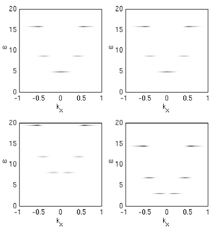
Figure 19: Spectral weight at $k_{y}=0$ for two vortex-lattice solutions. Left and right panels show left and right polarized components, respectively. Top: synchronized solution without a central vortex. ($J=0.5,\Delta=3.5,r_{0}=6.0$.) Bottom: desynchronized solution with a central vortex. ($J=0.5,\Delta=16.0,r_{0}=6.0$.)

VIII Conclusions

The interplay between the effects of pumping and decay in setting the density profile, and the dynamics of the polarization degree of freedom lead to a rich variety of possible nonequilibrium steady states, as well as dynamical attractors for the polarized polariton condensate in a harmonic trap. Even neglecting spatial currents, the two-mode model shows nontrivial behavior as a function of applied magnetic field: with strong damping there is a simple transition between synchronized and desynchronized states, whereas for weak damping, a region of bistability exists, in which the state established depends on the initial conditions.

Allowing for spatial fluctuations in a homogeneous system, the plane-wave modes on top of the synchronized solution show a second class of transition: if the phase locking term for the spin degree of freedom is large enough, then at weak magnetic fields, this term will provide sufficient restoring force for spin fluctuations to give underdamped global spin oscillations. As the magnetic field increases, the restoring force for such spin waves decreases, eventually vanishing when the synchronized solution becomes unstable. Before this instability occurs, there is a transition between underdamped and overdamped spin oscillations, and at this transition, the spin wave energies have a linear dispersion vs momentum.

Introducing vortices, the phase locking term favors co-alignment of vortices in the two spin polarizations, but at sufficiently large $\Delta$ anti-aligned vortex pairs may become stable. The phase-locking term also makes it possible to obtain a stationary complex of rarefaction waves. The experimental realization of such solitary vorticity-free waves would demonstrate another aspect of superfluid behaviorKeeling and Berloff (2009); Carusotto (2008) in the incoherently pumped polariton system.

Considering the transition between synchronized and desynchronized states in the inhomogeneous system, for sufficiently small pump spots, the transition is similar to the two-mode model. For larger pump spots however, an instability to vortex-lattice formation may preempt desynchronization, driven by the density imbalance required to sustain a synchronized solution. For both large and small pumping-spot radius, the phase portraits near the critical detuning can be more complicated, showing synchronized limit cycles with winding number 0, desynchronized limit cycles with winding number 2, and chaotic behavior.

In conclusion, the results presented here illustrate the wide variety of dynamical behavior that can arise in spinor polariton condensates, and suggest that experimental efforts to investigate such behavior should be feasible.

Appendix A Spiral vortices in the single component condensate

This appendix will discuss spiral vortices in the one-component version of Eq. (2), i.e., neglecting $J$ and $\Delta$. It was shown in Ref. Keeling and Berloff, 2008 that below the critical radius of pumping for the formation of a vortex lattice there exist states with one or a few spiral vortices. By combining vorticity with pumping and decay, one has both radial and azimuthal supercurrents, both of which modify the density profile, and so these currents interact. This is shown in Fig. 20, which shows both the radial velocity (main figure) for vortex solutions, and the density profile (inset). The vortex solution requires vanishing density at the origin, this makes the region at small radii a region of net gain, and leads to an outward-flowing current. Thus, in the vortex solutions, there exists both a local maximum of radial current, and a point at finite radius (of the order of the healing length) at which this current vanishes.

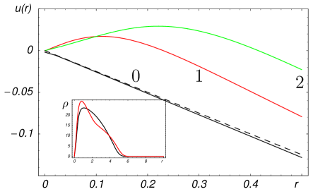
Figure 20: (Color online) Radial velocity, $u(r)=\phi^{\prime}(r)$, of the vortex solutions of Eq. (30) for $\alpha=1,\sigma=0.01$. The numbers next to the lines indicate the winding numbers of the vortices (1 and 2) and the ground state (0). The TF approximation of the gradient flow of the ground state for small $\alpha$ and $\sigma$ $u(r)=-r\sigma(\mu-r^{2})/6$, is given by the dashed line. The inset compares the density, $\rho(r)$, of a vortex solution for $\alpha=4,\sigma=0.27$ ($\mu=30.28$, gray (red) line) with the density of the GPE vortex ($\alpha=0,\sigma=0$) with the same number of particles ($2\pi\int|\psi|^{2}\,rdr=1000$, $\mu=25.68$, black line). Both vortex solutions have topological charge $1$.

In polar coordinates $(r,\theta)$ the wavefunction of a spiral vortex of topological charge $s$ in the one-component polariton condensate takes the form $\psi_{v}=f(r)\exp[i\phi(r)+s\theta]$, with the equations governing $f$ and $u(r)=\phi^{\prime}(r)$ given by

$$\begin{split}&\frac{d}{rdr}\Biggl{(}rf^{2}u\Biggr{)}=(\alpha\Theta(r_{0}-r)-\sigma f^{2})f^{2},\\ &f^{\prime\prime}+\frac{1}{r}f^{\prime}+\Biggl{(}\mu-u^{2}-\frac{s^{2}}{r^{2}}-f^{2}-r^{2}\Biggr{)}f=0.\end{split}$$ (30)

Around the center of the trap $f(r)$ and $u(r)$ can be found recursively in the form of the power series

$$f(r)=\sum_{i=1}^{\infty}a_{i}r^{|s|(2i-1)},\quad u(r)=\sum_{i=1}^{\infty}b_{i}r^{2i-1}.$$ (31)

To the leading order $u(r)\sim\alpha/2(s+1)r$ showing that the stronger the pumping the larger the outward velocity is in the vortex core. Only vortices of topological charge $1$ are dynamically stable. For these, $a_{1}\approx\delta\mu,a_{3}=-a_{1}\mu/8...,b_{2}=(\alpha\mu-8\sigma a_{1}^{2})/48...$, where the numerical value of the vortex core parameter $\delta\approx 0.583$ was first calculated by Pitaevskii Pitaevskii (1961) for the straight line vortex of uniform Gross–Pitaevskii condensate.

Appendix B Irregular vortex lattices

We note that around and above critical detuning, solutions to Eq. (2) may exhibit irregular density profiles and irregular vortex lattices. This happens most frequently when solutions are found starting from Gaussian initial conditions, but it may also happen for large $r_{0}$ when $\Delta$ is increased stepwise. As an example, we show a solution obtained from Gaussian initial conditions at $J=1.0,r_{0}=6.0,\Delta=6.0$ in Fig. 21. This solution shows an irregular vortex lattice, reminiscent of turbulent behavior.

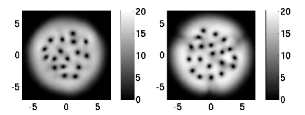
Figure 21: Density of the left- and right-polarized components, respectively, showing an irregular vortex lattice.

Appendix C Chemical potentials, phase portraits and numerical precession

In order to numerically find the chemical potential of a condensate with a rotating vortex lattice, it is useful to use:

$$\mu-2s\Omega=\frac{\int e^{is\vartheta}i\partial_{t}\psi(\mathbf{r})d^{2}r}{\int e^{is\vartheta}\psi(\mathbf{r})d^{2}r}$$ (32)

along with the equation:

$$\mu-2\langle L_{z}\rangle\Omega=\frac{\int\psi^{\ast}(\mathbf{r})i\partial_{t}\psi(\mathbf{r})d^{2}r}{\int|\psi(\mathbf{r})|^{2}d^{2}r}.$$ (33)

In many cases, Eq. (32) with $s=0$ is sufficient to determine $\mu$. However, when there is a vortex at the center of the cloud, the numerator and denominator both vanish, whereas one of $s=\pm 1$ will give a well defined value. In such cases, it is then necessary to use Eq. (33) and the integral for $\langle L_{z}\rangle$ to eliminate $\Omega$.

For plotting the phase portraits, it is necessary also to calculate the associated phase, $\phi$ such that $\dot{\phi}=\mu$. This can similarly be defined as:

$$\phi\equiv{\rm Im}\left\{\ln\left[\int\psi(\mathbf{r})\,d^{2}r\right]\right\}.$$ (34)

However, when there is a central vortex, the same difficulty will arise. To avoid this problem, two possible approaches are used. In some most cases it is sufficient to calculate $\dot{\theta}=\mu_{L}-\mu_{R}$, and numerically integrate this equation to find $\theta(t)$. Numerical errors in evaluating $\mu_{L,R}$ can however introduce unphysical precession into the plot of $\theta,\dot{\theta}$. To avoid this, in those cases where the nature of the portrait is simple, we use $\theta_{i+1}=\theta_{i}+\dot{\theta}\times dt\times f$, with $f\simeq 1$ adjusted to remove the spurious precession. This method has been used in Figs. 12, 13 (right hand panel) and 18.

Where the phase portrait involves finer structure, such as the middle panel of Fig. 13, the phase portrait has instead been obtained by:

$$\begin{split}\theta={\rm Im}&\left\{\ln\left[\int e^{is\vartheta}\psi_{R}(\mathbf{r})\,d^{2}r\right]\right.\\ &-\left.\ln\left[\int e^{is\vartheta}\psi_{L}(\mathbf{r})\,d^{2}r\right]\right\},\end{split}$$ (35)

with $s=0,\pm 1$ according to whether there is a central vortex. Since the two components are corotating in this case, such a definition satisfies:

$$\dot{\theta}=\left(\mu_{L}-2s\Omega\right)-\left(\mu_{R}-2s\Omega\right)=\mu_{L}-\mu_{R}$$ (36)

as required.

References

- Kasprzak et al. (2006) J. Kasprzak, M. Richard, S. Kundermann, A. Baas, P. Jeambrun, J. M. J. Keeling, F. M. Marchetti, M. H. Szymanska, R. Andre, J. L. Staehli, et al., Nature 443, 409 (2006).
- Balili et al. (2007) R. Balili, V. Hartwell, D. Snoke, L. Pfeiffer, and K. West, Science 316, 1007 (2007).
- Lagoudakis et al. (2008) K. G. Lagoudakis, M. Wouters, M. Richard, A. Baas, I. Carusotto, R. Andre, L. S. Dang, and B. Devaud-Plédran, Nature Phys. 4, 706 (2008).
- Utsunomiya et al. (2008) S. Utsunomiya, L. Tian, G. Roumpos, C. W. Lai, N. Kumada, T. Fujisawa, M. Kuwata-Gonokami, A. Löffler, S. Höfling, A. Forchel, et al., Nature Phys. 4, 700 (2008).
- Amo et al. (2009a) A. Amo, D. Sanvitto, F. P. Laussy, D. Ballarini, E. del Valle, M. D. Martin, A. Lemaître, J. Bloch, D. N. Krizhanovskii, M. S. Skolnick, et al., Nature 457, 291 (2009a).
- Amo et al. (2009b) A. Amo, J. Lefrére, S. Pigeon, C. Adrados, C. Ciuti, I. Carusotto, R. Houdré, E. Giacobino, and A. Bramati, Nature Phys. (2009b).
- Demokritov et al. (2006) S. O. Demokritov, V. E. Demidov, O. Dzyapko, G. A. Melkov, A. A. Serga, B. Hillebrands, and A. N. Slavin, Nature 443, 430 (2006).
- Demidov et al. (2008) V. E. Demidov, O. Dzyapko, S. O. Demokritov, G. A. Melkov, and A. N. Slavin, Phys. Rev. Lett. 100, 047205 (2008).
- Chumak et al. (2009) A. V. Chumak, G. A. Melkov, V. E. Demidov, O. Dzyapko, V. L. Safonov, and S. O. Demokritov, Phys. Rev. Lett. 102, 187205 (2009).
- Dzyapko et al. (2009) O. Dzyapko, V. E. Demidov, M. Buchmeier, T. Stockhoff, G. Schmitz, G. A. Melkov, and S. O. Demokritov, Phys. Rev. B 80, 060401(R) (2009).
- Volovik (2008) G. Volovik, J. Low. Temp. Phys. 153, 266 (2008).
- Ciuti et al. (2003) C. Ciuti, P. Schwendimann, and A. Quattropani, Semicond. Sci. Technol. 18, S279 (2003).
- Keeling et al. (2007) J. Keeling, F. M. Marchetti, M. H. Szymańska, and P. B. Littlewood, Semicond. Sci. Technol. 22, R1 (2007).
- Kavokin et al. (2007) A. V. Kavokin, J. J. Baumberg, G. Malpuech, and F. P. Laussy, Microcavities (Oxford Univeristy Press, Oxford, 2007).
- Laussy et al. (2006) F. P. Laussy, I. A. Shelykh, G. Malpuech, and A. Kavokin, Phys. Rev. B 73, 035315 (2006).
- Shelykh et al. (2006) I. A. Shelykh, Y. G. Rubo, G. Malpuech, D. D. Solnyshkov, and A. Kavokin, Phys. Rev. Lett. 97, 066402 (2006).
- Rubo et al. (2006) Y. G. Rubo, A. V. Kavokin, and I. A. Shelykh, Phys. Lett. A 358, 227 (2006).
- Keeling (2008) J. Keeling, Phys. Rev. B 78, 205316 (2008).
- Rubo (2007) Y. G. Rubo, Phys. Rev. Lett. 99, 106401 (2007).
- Lagoudakis et al. (2009) K. G. Lagoudakis, T. Ostatnicky, A. V. Kavokin, Y. G. Rubo, R. Andre, and B. Deveaud-Pledran, Science 326, 974 (2009).
- Panzarini et al. (1999) G. Panzarini, L. C. Andreani, A. Armitage, D. Baxter, M. S. Skolnick, V. N. Astratov, J. S. Roberts, A. V. Kavokin, M. R. Vladimirova, and M. A. Kaliteevski, Phys. Rev. B 59, 5082 (1999).
- Toledo Solano and Rubo (2009) M. Toledo Solano and Y. G. Rubo (2009), arXiv:0910.2727.
- Aleiner and Ivchenko (1992) I. L. Aleiner and E. L. Ivchenko, JETP Lett. 55, 692 (1992).
- Malpuech et al. (2006) G. Malpuech, M. M. Glazov, I. A. Shelykh, P. Bigenwald, and K. V. Kavokin, Appl. Phys. Lett. 88, 111118 (2006).
- (25) D. W. Snoke, Private communication.
- Amo et al. (2005) A. Amo, M. D. Martín, D. Ballarini, L. Viña, D. Sanvitto, M. S. Skolnick, and J. S. Roberts, Phys. Stat. Sol. (c) 2, 3868 (2005).
- Klopotowski et al. (2006) L. Klopotowski, M. Martín, A. Amo, L. Viña, I. Shelykh, M. Glazov, G. Malpuech, A. Kavokin, and R. André, Solid State Commun. 139, 511 (2006).
- Kasprzak et al. (2007) J. Kasprzak, R. André, L. S. Dang, I. A. Shelykh, A. V. Kavokin, Y. G. Rubo, K. V. Kavokin, and G. Malpuech, Phys. Rev. B 75, 045326 (2007).
- Leggett (2001) A. J. Leggett, Rev. Mod. Phys. 73, 307 (2001).
- Shelykh et al. (2008) I. A. Shelykh, D. D. Solnyshkov, G. Pavlovic, and G. Malpuech, Phys. Rev. B 78, 041302(R) (2008).
- Satija et al. (2009) I. I. Satija, R. Balakrishnan, P. Naudus, J. Heward, M. Edwards, and C. W. Clark, Phys. Rev. A 79, 033616 (2009).
- Juliá-Díaz et al. (2009) B. Juliá-Díaz, M. Melé-Messeguer, M. Guilleumas, and A. Polls, Phys. Rev. A 80, 043622 (2009).
- Wouters (2008) M. Wouters, Phys. Rev. B 77, 121302(R) (2008).
- Eastham (2008) P. R. Eastham, Phys. Rev. B 78, 035319 (2008).
- Keeling and Berloff (2008) J. Keeling and N. G. Berloff, Phys. Rev. Lett. 100, 250401 (2008).
- Wouters et al. (2008) M. Wouters, I. Carusotto, and C. Ciuti, Phys. Rev. B 77, 115340 (2008).
- Wouters and Savona (2009) M. Wouters and V. Savona, Phys. Rev. B 79, 165302 (2009).
- Aranson and Kramer (2002) I. S. Aranson and L. Kramer, Rev. Mod. Phys. 74, 99 (2002).
- Staliunas and Sanchez-Morcillo (2003) K. Staliunas and V. J. Sanchez-Morcillo, Transverse Patterns in Nonlinear Optical Resonators, vol. 183 of Springer Tracts in Modern Physics (Springer-Verlag, Berlin, 2003).
- Michinel et al. (2002) H. Michinel, J. Campo-Táboas, R. García-Fernández, J. R. Salgueiro, and M. L. Quiroga-Teixeiro, Phys. Rev. E 65, 066604 (2002).
- Michinel et al. (2006) H. Michinel, M. J. Paz-Alonso, and V. M. Pérez-García, Phys. Rev. Lett. 96, 023903 (2006).
- Wouters and Carusotto (2007a) M. Wouters and I. Carusotto, Phys. Rev. Lett. 99, 140402 (2007a).
- Szymańska et al. (2006) M. H. Szymańska, J. Keeling, and P. B. Littlewood, Phys. Rev. Lett. 96, 230602 (2006).
- Szymańska et al. (2007) M. H. Szymańska, J. Keeling, and P. B. Littlewood, Phys. Rev. B 75, 195331 (2007).
- Wouters and Carusotto (2006) M. Wouters and I. Carusotto, Phys. Rev. B 74, 245316 (2006).
- Wouters and Carusotto (2007b) M. Wouters and I. Carusotto, Phys. Rev. A 76, 043807 (2007b).
- Renucci et al. (2005) P. Renucci, T. Amand, X. Marie, P. Senellart, J. Bloch, B. Sermage, and K. V. Kavokin, Phys. Rev. B 72, 075317 (2005).
- Strogatz (1994) S. H. Strogatz, Nonlinear dynamics and chaos (Perseus Books, Cambridge, Mass., 1994).
- Urabe (1955) M. Urabe, J. Sci. Hiroshima Univeristy A 18, 379 (1955).
- Jones and Roberts (1982) C. A. Jones and P. H. Roberts, Journal of Physics A: Mathematical and General 15, 2599 (1982).
- Mason and Berloff (2008) P. Mason and N. G. Berloff, Phys. Rev. A 77, 032107 (2008).
- Rubinstein and Pismen (1994) B. Rubinstein and L. M. Pismen, Physica D 78, 1 (1994).
- Kivshar et al. (1998) Y. S. Kivshar, J. Christou, V. Tikhonenko, B. Luther-Davies, and L. M. Pismen, Opt. Commun. 152, 198 (1998).
- Khandekar and Rao (1975) M. L. Khandekar and G. V. Rao, Meteorology and Atmospheric Physics 24, 19 (1975).
- Richard et al. (2005) M. Richard, J. Kasprzak, R. André, R. Romestain, L. S. Dang, G. Malpuech, and A. Kavokin, Phys. Rev. B 72, 201301(R) (2005).
- Tilley and Tilley (1990) D. R. Tilley and J. Tilley, Superfluidity and Superconductivity (IOP Publishing Ltd, Bristol, UK, 1990), 3rd ed.
- Keeling and Berloff (2009) J. Keeling and N. G. Berloff, Nature 457, 273 (2009).
- Carusotto (2008) I. Carusotto, The meaning of superfluidity for polariton condensates, Presentation at ICSCE4 (2008), URL http://www.tcm.phy.cam.ac.uk/BIG/icsce4/talks/carusotto.pdf.
- Pitaevskii (1961) L. P. Pitaevskii, Sov. Phys. JETP 13, 451 (1961).