An Equation of State of a Carbon-Fibre Epoxy Composite under Shock Loading

Abstract

An anisotropic equation of state (EOS) is proposed for the accurate extrapolation of high-pressure shock Hugoniot (anisotropic and isotropic) states to other thermodynamic (anisotropic and isotropic) states for a shocked carbon-fibre epoxy composite (CFC) of any symmetry. The proposed EOS, using a generalised decomposition of a stress tensor [Int. J. Plasticity 24, 140 (2008)], represents a mathematical and physical generalisation of the Mie-Grüneisen EOS for isotropic material and reduces to this equation in the limit of isotropy. Although a linear relation between the generalised anisotropic bulk shock velocity $U^{A}_{s}$ and particle velocity $u_{p}$ was adequate in the through-thickness orientation, damage softening process produces discontinuities both in value and slope in the $U^{A}_{s}$-$u_{p}$ relation. Therefore, the two-wave structure (non-linear anisotropic and isotropic elastic waves) that accompanies damage softening process was proposed for describing CFC behaviour under shock loading. The linear relationship $U^{A}_{s}$-$u_{p}$ over the range of measurements corresponding to non-linear anisotropic elastic wave shows a value of $c^{A}_{0}$ (the intercept of the $U^{A}_{s}$-$u_{p}$ curve) that is in the range between first and second generalised anisotropic bulk speed of sound [Eur. Phys. J. B 64, 159 (2008)]. An analytical calculation showed that Hugoniot Stress Levels (HELs) in different directions for a CFC composite subject to the two-wave structure (non-linear anisotropic elastic and isotropic elastic waves) agree with experimental measurements at low and at high shock intensities. The results are presented, discussed and future studies are outlined.

I Introduction

Investigation of anisotropic composite materials (e.g., CFC materials) behaviour has found significant interest in the research community due to the widespread application of anisotropic composite materials in aerospace and civil engineering problems. Modern high-resolution methods for monitoring the stress and particle velocity histories in shock waves and equipment have been created BarkerHollenbach (1, 2, 3, 4, 5). A common technique for the study of material behaviour under shock loading is the planar plate impact test (one-dimensional shock wave propagation). Shock wave experiments have frequently provided the motivation for the construction of material constitutive relations and have been the principal means for determining material parameters for some of these relations DavisonGraham (6, 7, 8, 9, 10). For example, Dandekar et al. Dandekaretal (11) investigated the equation of state of a glass fibre epoxy composite, in terms of the shock stress, shock velocity $U_{s}$ (through-thickness orientation) and particle velocity $u_{p}$ (i.e. the velocity of material flow behind the shock front). Their results indicated that there was a linear relationship between shock and particle velocity. This type of behaviour is typical of a wide range of materials, including metals Meyers (8, 9) and some polymers, including epoxy resins MunsonMay (12, 13), and composite Zhuketal (14), including carbon fibre epoxy composite Riedeletal (15) and glass fibre epoxy composite Zaretskyetal (16). A linear $U_{s}$-$u_{p}$ relationship shows that in the through thickness orientation, this class of composite displays fairly typical experimental data. However, in spite of a perfectly adequate general understanding, experimental methodology, and theory, material models do not agree in detail, especially for anisotropic composite materials. For many years, it has been assumed that the response of composite materials to shock loading is isotropic Chenetal (17, 18, 19), and only recently has anisotropy in the shock response of anisotropic materials (e.g., composite materials) attracted the attention of researchers Andersonetal2 (20, 21, 22), MillettLukyanov (23, 24, 25, 26).

In this paper, a macroscopic continuum framework is chosen to modify the existing methodology for accurate extrapolation of high-pressure shock Hugoniot states to other thermodynamic states for a shocked isotropic continuum. The composite materials response under shock loading leads to a nonlinear behavior (i.e. large compressions), therefore, an equation of state (EOS) is required Andersonetal1 (19, 24, 25, 26). To address this issue, an anisotropic equation of state similar to Lukyanov2 (24, 25, 26) is proposed for accurate extrapolation of high-pressure shock Hugoniot (anisotropic and isotropic) states to other thermodynamic (anisotropic and isotropic) states for a shocked carbon-fibre epoxy composite of any symmetry.

II An anisotropic Equation of State

The proposed equation of state, using the generalised decomposition of a stress tensor Lukyanov2 (24, 25, 26, 27, 28), represents a mathematical and physical generalisation of the Mie-Grüneisen equation of state for isotropic material and reduces to this equation in the limit of isotropy. The generalised decomposition of the stress tensor is summarised below. The generalised decomposition framework will provide a useful point of construction of an anisotropic equation of state.

II.1 Generalised decomposition of the stress tensor: $\alpha$-$\beta$ decomposition

The definition of pressure in the case of an anisotropic solids should be the result of stating that the ”pressure” term should only produce a change of scale, i.e. isotropic state of strain Lukyanov2 (24, 25, 26, 27, 28). The generalised decomposition of the stress tensor $\sigma_{ij}$ is defined as:

$$\tilde{{\rm P}}:\tilde{S}=0\quad\mbox{or}\quad\alpha_{ij}\tilde{S}_{ij}=0,\quad\sigma_{ij}=-p^{\ast}\alpha_{ij}+\tilde{S}_{ij},$$ (1)

where $\tilde{{\rm P}}=p^{\ast}\alpha_{ij}$ is the generalised spherical part of the stress tensor, $\tilde{S}=\tilde{S}_{ij}$ is the generalised deviatoric stress tensor, $p^{\ast}$ is the total generalised ”pressure” and $\alpha_{ij}$ is the first generalisation of the Kronecker delta symbol. The constructive definition of the tensor $\alpha_{ij}$ is based on the fact that the stress tensor $p\alpha_{ij}$ is induced in the anisotropic medium by the applied isotropic strain tensor $\displaystyle\frac{\varepsilon_{v}}{3}\delta_{ij}$, i.e.

$$p\alpha_{ij}=-\frac{\varepsilon_{v}}{3}\textbf{C}_{ijkl}\delta_{kl},\quad p=-K_{C}\varepsilon_{v},$$ (2)

where $p$ is the pressure, $\varepsilon_{v}$ is the volumetric strain, $\delta_{ij}$ is the Kronecker delta symbol (unit tensor), $\textbf{C}_{ijkl}$ is the elastic stiffness matrix and $K_{C}$ is the first generalised bulk modulus. The expressions for the $\alpha_{ij}$ components and $K_{C}$ are presented below. Throughout, the contraction by repeating indexes is assumed. Using (1), the following expression for total generalised ”pressure” $p^{\ast}$ can be obtained:

$$p^{\ast}=-\frac{{\sigma_{ij}\alpha_{ij}}}{{\alpha_{kl}\alpha_{kl}}}=-\frac{{1}}{{\left\|{\alpha}\right\|^{2}}}\sigma_{ij}\alpha_{ij},$$ (3)

where $\left\|{\alpha}\right\|^{2}=\alpha_{ij}\alpha_{ij}=\alpha_{11}^{2}+\alpha_{22}^{2}+\alpha_{33}^{2}$. Finally, the expression for the generalised deviatoric part of the stress tensor can be rewritten in the following form:

$$\tilde{S}_{ij}=\sigma_{ij}-\alpha_{ij}\cdot\frac{{1}}{{\left\|{\alpha}\right\|^{2}}}\sigma_{kl}\alpha_{kl}.$$ (4)

For anisotropic materials, the total generalised ”pressure” $p^{*}$ has been expressed Lukyanov2 (24, 25, 26, 27, 28) as:

$$p^{*}=p+p^{\tilde{S}},\ p=-\frac{\beta_{ij}\sigma_{ij}}{\beta_{ij}\alpha_{ij}},\ p^{\tilde{S}}=\ \frac{{\beta_{ij}\tilde{S}_{ij}}}{{\beta_{kl}\alpha_{kl}}},$$ (5)

where $p$ is the pressure related to the volumetric deformation (2), $p^{\tilde{S}}$ is the pressure related to the generalised deviatoric stress and $\beta_{ij}$ is the second generalisation of the Kronecker delta symbol. The constructive definition of the tensor $\beta_{ij}$ is based on the fact that stress tensor $p\beta_{ij}$ is independent of the stress tensor $\textbf{C}_{ijkl}e_{kl}$, i.e. their contraction product is zero for any deviatoric strain tensor $e_{kl}$, where $\textbf{C}_{ijkl}$ is the elastic stiffness matrix. The following relation describes the functional definition of the second order material tensor $\beta_{ij}$:

$$\beta_{ij}\textbf{C}_{ijkl}=3K_{S}\delta_{kl},$$ (6)

where $K_{S}$ represents the second generalised bulk modulus. The solution of equations (6) in terms of the $\beta_{ij}$ components and an expression for $K_{S}$ are presented below. Equations (5) define the correct generalised ”pressure” for the elastic regime. Note that the generalised decomposition of the stress tensor can be applied for all anisotropic solids of any symmetry and represents a mathematically consistent generalisation of the conventional isotropic case. The procedure of construction for the tensor $\alpha_{kl}$ has been defined in Lukyanov2 (24, 25, 26, 27, 28). The elements of the tensor $\alpha_{kl}$ are

$$\begin{array}[]{*{20}c}\displaystyle\alpha_{11}=\left(\sum^{3}_{k=1}C_{k1}\right)\cdot 3\bar{K}_{C},\ \alpha_{22}=\left(\sum^{3}_{k=1}C_{k2}\right)\cdot 3\bar{K}_{C},\hfill\\ \displaystyle\alpha_{33}=\left(\sum^{3}_{k=1}C_{k3}\right)\cdot 3\bar{K}_{C},\ \alpha_{ij}\alpha_{ij}=3,\hfill\end{array}$$ (7)

$$\begin{array}[]{*{20}c}\displaystyle K_{C}=\frac{1}{3\sqrt{3}}\sqrt{\left(\sum^{3}_{k=1}C_{k1}\right)^{2}+\left(\sum^{3}_{k=1}C_{k2}\right)^{2}+\left(\sum^{3}_{k=1}C_{k3}\right)^{2}},\hfill\\ \displaystyle K_{C}=\frac{1}{9\bar{K}_{C}},\hfill\end{array}$$ (8)

where $C_{ij}$ is the elastic stiffness matrix (written in Voigt notation). The elements of the tensor $\beta_{kl}$ are

$$\begin{array}[]{*{20}c}\displaystyle\beta_{11}=\left(\sum^{3}_{k=1}J_{k1}\right)\cdot 3K_{S},\ \beta_{22}=\left(\sum^{3}_{k=1}J_{k2}\right)\cdot 3K_{S},\hfill\\ \displaystyle\beta_{33}=\left(\sum^{3}_{k=1}J_{k3}\right)\cdot 3K_{S},\ \beta_{ij}\beta_{ij}=3,\hfill\end{array}$$ (9)

$$\frac{1}{K_{S}}=\sqrt{3}\sqrt{\left(\sum^{3}_{k=1}J_{k1}\right)^{2}+\left(\sum^{3}_{k=1}J_{k2}\right)^{2}+\left(\sum^{3}_{k=1}J_{k3}\right)^{2}},$$ (10)

where $J_{ij}$ are elements of the compliance matrix (written in Voigt notation). In the limit of isotropy, the proposed generalisation returns to the traditional classical case where tensors $\alpha_{ij}$ and $\beta_{ij}$ equal $\delta_{ij}$ and equations (5) take the form:

$$\begin{array}[]{*{20}c}\displaystyle p^{\ast}=-\frac{{\sigma_{ij}\delta_{ij}}}{{\delta_{kl}\delta_{kl}}}=-\frac{{1}}{{3}}\sigma_{kk}\hfill\\ \displaystyle p=-\frac{{\beta_{ij}\sigma_{ij}}}{{\beta_{kl}\alpha_{kl}}}=-\frac{{1}}{{3}}\sigma_{kk},\hfill\\ \displaystyle p^{\tilde{S}}=\ \frac{{\beta_{ij}\tilde{S}_{ij}}}{{\beta_{kl}\alpha_{kl}}}=0,\hfill\end{array}$$ (11)

where $\displaystyle p=-\frac{\sigma_{kk}}{3}$ is the classical hydrostatic pressure. Also, parameters $K_{C}$ and $K_{S}$ were considered as the first and the second generalised bulk moduli. In the limit of isotropy, they reduce to the well-know expression for conventional bulk modulus.

The geometrical representation of generalized decomposition of the stress can be shown in the principal stress space (Haigh-Westergaard stress space) for $\alpha$-decomposition of the stress tensor and $\beta$-decomposition of the stress tensor in the principal strain space. Figure 1 shows schematic representation of $\alpha$-decomposition of the stress tensor, where $\alpha$-direction is described by the tensor $\alpha_{ij}$ and $\delta$-direction is described by the Kronecker’s delta tensor $\delta_{ij}$. Therefore, $p_{\delta}$ describes the hydrostatic stress (isotropic stress), $p^{\ast}\neq p_{\delta}$ describes the total generalized hydrostatic stress (or anisotropic total generalized hydrostatic stress), and $p\neq p^{\ast}\neq p_{\delta}$ is the generalized pressure related to an equation of state (EOS). The angle between $\alpha$-direction and $\delta$-direction is described by the variable $\psi$ which can be obtained from $\displaystyle\cos\psi=\frac{\alpha_{11}+\alpha_{22}+\alpha_{33}}{3}$. Similar representation can be shown for $\beta$-decomposition of the stress tensor (Haigh-Westergaard stress space).

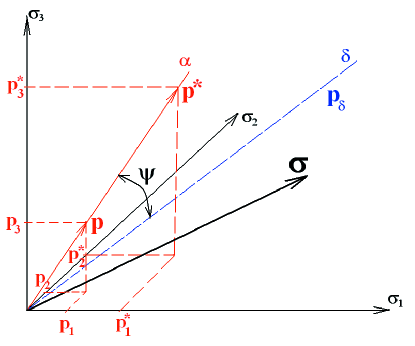
Figure 1: Schematic representation of $\alpha$-decomposition of the stress tensor (Haigh-Westergaard stress space).

II.2 An anisotropic EOS

The equations (5) define the correct generalised ”pressure” for the elastic regime:

$$p^{*}=p+\frac{{\beta_{ij}\tilde{S}_{ij}}}{{\beta_{kl}\alpha_{kl}}},\ \sigma_{ij}=-p^{*}\alpha_{ij}+\tilde{S}_{ij}.$$ (12)

Further, to provide an appropriate description for general anisotropic materials behavior at high pressures, the pressure $p$ related to the volumetric deformations is described by the Mie-Grüneisen equation of state pressure $p^{EOS}$:

$$p=p^{EOS}=f\left({\rho,e}\right)=P^{A}_{H}\cdot\left({1-\frac{{\Gamma}}{{2}}\mu}\right)+\rho\Gamma e$$ (13)

or

$$p^{EOS}=\left\{{{\begin{array}[]{*{20}c}\displaystyle{\frac{{\rho_{0}\left(c^{A}_{0}\right)^{2}\mu\left[{1+\left({1-\frac{{\Gamma(\nu)}}{{2}}}\right)\mu-\frac{{\Gamma(\nu)}}{{2}}\mu^{2}}\right]}}{{\left[{1-\left({S^{A}_{1}-1}\right)\mu-S^{A}_{2}\frac{{\mu^{2}}}{{\mu+1}}-S^{A}_{3}\frac{{\mu^{3}}}{{\left({\mu+1}\right)^{2}}}}\right]^{2}}}}+\hfill\\ {+\left({1+\mu}\right)\cdot\Gamma(\nu)\cdot E,\quad\mu>0;\hfill}\\ {\rho_{0}\left(c^{A}_{0}\right)^{2}\mu+\left({1+\mu}\right)\cdot\Gamma\cdot E,\quad\mu<0;\hfill}\\ \end{array}}}\right.,$$ (14)

$$\Gamma(\nu)=\frac{{\gamma_{0}+a\mu}}{{1+\mu}},\ \displaystyle\mu=\frac{{\rho}}{{\rho_{0}}}-1,$$ (15)

where $\gamma_{0}$ is the initial Grüneisen gamma, $a$ is the first order volume correction to $\gamma_{0}$, $P^{A}_{H}$ is the anisotropic generalised bulk Hugoniot pressure, $E$ is the internal energy per initial density $\displaystyle\left(E=\frac{e}{\rho_{0}}\right)$, $\mu$ is the relative change of volume, $\nu$ is the specific volume and $S^{A}_{1}$, $S^{A}_{2}$, $S^{A}_{3}$ are the intercept of the cubic $U^{A}_{s}$-$u_{p}$ curve Steinberg (9):

$$U^{A}_{s}=c^{A}_{0}+S^{A}_{1}u_{p}+S^{A}_{2}\left({\frac{{u_{p}}}{{U^{A}_{s}}}}\right)u_{p}+S^{A}_{3}\left({\frac{{u_{p}}}{{U^{A}_{s}}}}\right)^{2}u_{p},$$ (16)

where $U^{A}_{s}$ is the generalised anisotropic bulk shock velocity and $c^{A}_{0}$ is the velocity curve intercept. The proposed generalised ”pressure” also correctly describes the medium behavior at small volumetric strains. To be consistent with the definition of the isotropic bulk speed of sound, the following definitions of the first $c_{I}$ and the second $c_{II}$ bulk speed of sound for anisotropic medium are assumed Lukyanov3 (25):

$$c_{I}=\sqrt{\frac{K_{C}}{\rho_{0}}},\ c_{II}=\sqrt{\frac{K_{S}}{\rho_{0}}},$$ (17)

where the generalised bulk moduli $K_{C}$, $K_{S}$ are defined according to (8) and (10) respectively. Parameters $c^{A}_{0}\in[c_{II},c_{I}]$, $S^{A}_{1}$, $S^{A}_{2}$, $S^{A}_{3}$, $\gamma_{0}$, $a$ represent material properties which define its EOS (14).

III The behaviour of a Carbon-Fibre Epoxy Composite under shock loading

The purpose of this section is to display the accurate extrapolation of experimental Hugoniot states MillettLukyanov (23) behind the shock wave (thermodynamic states) to high-pressure shock Hugoniot Stress Levels (HSLs) for a shocked carbon-fibre epoxy composite (initially anisotropic CFC) using the anisotropic EOS proposed above.

III.1 Description of Experiment

The work discussed below concerns the shock response of a carbon-fibre epoxy composite. This is done by the technique of plate impact, whereby a flat plate of constant thickness and of known material (for instance aluminium alloy, or copper) is impacted onto a target plate made from the test material. The flyer plates are launched using a $50\ mm$ bore, $5\ m$ long single stage gas gun. The plate impact test was done at the Defence Academy of the United Kingdom by Millett et al. MillettLukyanov (23) using samples of a carbon-fibre composite (CFC) of thicknesses $3.8\ mm$. The impact axises were (a) normal to the plane of the fibres and (b) parallel to the plane of the fibres. On impact, a planar shock front starts propagating into the target. The shock propagation in the target is monitored using manganin stress gauges, placed at different locations within the target assembly. A schematic of the target assembly and gauge placement is shown in Figure 2. A manganin stress gauge was supported on the back of the specimen plate with a $12\ mm$ block of polymethylmethacrylate (PMMA). Also, the gauge was backed into the PMMA by approximately $1.5\ mm$ PMMA offset block to act as extra protection for the gauge. A second gauge (the $0\ mm$ position) was supported on the front of the target assembly with a $1\ mm$ plate of aluminium alloy 6082-T6. Shock stresses were induced with dural flyer plates impacting with the different velocities, using a single stage gas gun MillettLukyanov (23).

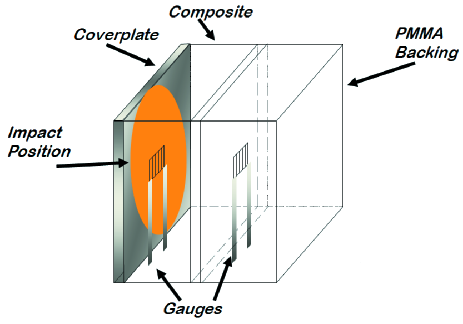
Figure 2: Target assembly.

The results from the stress gauges were converted to material (Target) values $\sigma_{M}$, using the shock impedances of the target $A_{T}$ and PMMA $A_{P}$, via the well-known relation Meyers (8, 13, 23):

$$\sigma_{M}=\frac{A_{T}+A_{P}}{2A_{P}}\sigma_{P},$$ (18)

where $\sigma_{P}$ is the stress gauges values. Furthermore, temporary spacing $(\delta t)$ between the tracers in combination with the specimen thickness $(\delta w)$ were used to obtain the shock velocities in the longitudinal (through thickness orientation $U^{L}_{s}=\delta w/\delta t$ and along the fibre $0^{o}$ orientation $U^{F}_{s}=\delta w/\delta t$, taking into account both the offset distance of the gauge within the PMMA and the known shock response of PMMA BarkerHollenbach (1), MillettLukyanov (23).

III.2 Materials

The fibres in the carbon-fibre epoxy composite were Hexcel 5HS in a woven lay up of orientation $[0/90,\pm 45]_{4}$. The arial weight was $370\ g/m^{2}$. The resin was an epoxy, Hexcel RTM6. The composite was cured at $180^{o}\ C$ under a pressure of $100\ psi$ ($6.7\ atm$) for 1 hour 40 minutes. The microstructure is shown in Fig. (3). The longitudinal sound speed in the through-thickness orientation $C_{L}$ was $3020\ m/s$, and the ambient density $\rho$ was $1.50\ g/cm^{3}$.

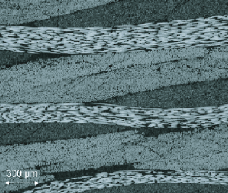
Figure 3: Microstructure of carbon-fibre epoxy composite.

The equivalent material properties of the CFC composite plate were chosen to match the layer macromechanical properties for the layup $[0/90,\pm 45]_{4}$ only and the longitudinal sound speed in the through-thickness orientation. A description of their numerical values for the selected Carbon Fibre Composite (CFC) is shown in Table 1.

Table 1: Material properties of undamaged (CFC) Carbon Fibre Composite (11-direction corresponds to the fill direction, 22-direction to the warp direction and 33-direction the through-thickness orientation).

Parameter	Description	CFC
$\rho^{A}_{0}\ \left[kg/m^{3}\right]$	Density	1500.0
$E_{1}\left[GPa\right]$	Elastic modulus (22 direction)	68.467
$E_{2}\left[GPa\right]$	Elastic modulus (11 direction)	66.537
$E_{3}\left[GPa\right]$	Elastic modulus (33 direction)	13.678
$K_{C}\left[GPa\right]$	Firtst generalised bulk modulus	19.436
$K_{S}\left[GPa\right]$	Second generalised bulk modulus	7.6902
$C_{L}\ \left[m/s\right]$	Sound speed (11 direction)	6762.0
$C_{L}\ \left[m/s\right]$	Sound speed (22 direction)	6666.0
$C_{L}\ \left[m/s\right]$	Sound speed (33 direction)	3020.0
$\nu_{21}$	Poisson’s ratio	0.0400
$\nu_{31}$	Poisson’s ratio	0.0045
$\nu_{32}$	Poisson’s ratio	0.0044
$\alpha^{A}_{11}$	Tensor $\alpha$ (22 direction)	1.2290
$\alpha^{A}_{22}$	Tensor $\alpha$ (11 direction)	1.1956
$\alpha^{A}_{33}$	Tensor $\alpha$ (33 direction)	0.2454
$\beta^{A}_{11}$	Tensor $\beta$ (22 direction)	0.3155
$\beta^{A}_{22}$	Tensor $\beta$ (11 direction)	0.3254
$\beta^{A}_{33}$	Tensor $\beta$ (33 direction)	1.6717

The acoustic longitudinal speed of sound in the through-thickness orientation is:

$$C_{L}=\sqrt{\left(\frac{1}{\rho}\frac{\partial\sigma_{L}}{\partial\varepsilon_{L}}\right)_{\rho=\rho_{0}}},$$ (19)

where $\sigma_{L}$ is the longitudinal stress, $\varepsilon_{L}$ is the longitudinal strain. Using the generalised Hook law for orthotropic materials and an uniaxial acoustic strain state (through thickness orientation), i.e. $\varepsilon_{L}=\varepsilon_{33}=\varepsilon_{zz}$ ($\varepsilon_{ij}\neq 0\ i,j=3$ only), the longitudinal speed of sound (through thickness orientation) (19) takes the form:

$$C_{L}=\sqrt{\frac{1}{\rho_{0}}\left[\frac{\left(1-\nu_{12}\nu_{21}\right)E_{3}}{\Delta}\right]},$$ (20)

where $\Delta=\left(1-\nu_{12}\nu_{21}-\nu_{23}\nu_{32}-\nu_{31}\nu_{13}-2\nu_{21}\nu_{32}\nu_{13}\right)$; $E_{1}$, $E_{2}$, $E_{3}$ are Young’s moduli and $\nu_{ij}$ are Poisson ratios. The measured longitudinal speed of sound was $C_{L}=3020\pm 30\ m/s$ for the initial material density $\rho_{0}=1500\pm 10\ kg/m^{3}$ MillettLukyanov (23). Using (20) and elastic material properties in Table 1, the longitudinal speed of sound is calculated to be $C_{L}=3020\ m/s$, which is in exact agreement with the measured value of $3020\pm 30\ m/s$. Note that we have a six elastic unknown material properties listed in Table 1, which directly affect shock waves propagation under uniaxial strain state. However, only one longitudinal sound speed in the through-thickness orientation, depending on four unknown elastic properties, was experimentally measured MillettLukyanov (23). Hence, the equivalent material properties given in Table 1 have not been finalised yet for the selected CFC material.

III.3 Results and discussion

Initially, the equations of state, in terms of the shock and particle velocities, are examined. Although a linear relationship in the $U^{A,L,F}_{s}$-$u_{p}$ plane is adequate for simple materials and some anisotropic metals Lukyanov2 (24, 25, 26, 29), phase changes under shock loading (e.g., damage softening) produce discontinuities both in value and slope in the $U^{A,L,F}_{s}$-$u_{p}$ relation, where $U^{A,L,F}_{s}$ (i.e., $U^{A}_{s}$, $U^{L}_{s}$, $U^{F}_{s}$) represent the generalised shock velocities in the directions of anisotropic bulk, longitudinal through-thickness, and along the fibre $0^{o}$ orientation, respectively. These discontinuities are usually caused by the two-wave structure that accompanies most phase changes, as well as damage softening. It was pointed out by Bethe Bethe (30) that, for stable shock waves, the shock velocity must increase with pressure. This means that if the shock velocity should decrease with pressure, then the shock front would break up into two or more waves, or possibly one wave with a continuously smeared front.

Note that the experimental data for the through thickness orientation (see, Fig. (4)) can be fitted by a linear relation, and there is no explicit evidence of the shock front breaking up; however, the analysis of the experimental data for selected CFC material MillettLukyanov (23) (see, Fig. (4)) shows that the shock velocity along the fibre $0^{o}$ orientation decreases with pressure – therefore, a two-wave structure is proposed for describing the experimental data. Additionally, a comparison of the equations of state in terms of Hugoniot Stress Levels (HSLs) for the single wave and two-wave structures is performed, in order to demonstrate the accuracy of the two-wave structure methodology. As a result, the experimental data MillettLukyanov (23) for longitudinal (through thickness) orientation and along the fibre $0^{o}$ orientation shock wave propagation in the selected CFC material has been fitted by straight lines (for single wave and two-wave structures), that is, using relationships for $U^{L}_{s}$-$u_{p}$ and $U^{F}_{s}$-$u_{p}$ that are linear (see, Figs. (4), (6)).
For a single wave structure:

$$\begin{array}[]{*{20}c}\displaystyle a)\ U^{L}_{s}=c^{L}_{0}+S^{L}_{1}u_{p},\ c^{L}_{0},\ S^{L}_{1}>0,\ \forall\ u_{p},\hfill\\ \displaystyle b)\ U^{F}_{s}=c^{F}_{0}+S^{F}_{1}u_{p},\ c^{F}_{0},\ S^{F}_{1}>0,\ \forall\ u_{p},\end{array}$$ (21)

and, for a two-wave structure:

$$\begin{array}[]{*{20}c}\displaystyle c)\ U^{L}_{s}=\left\{\begin{array}[]{*{20}c}\displaystyle c^{AL}_{0}+S^{AL}_{1}u_{p},c^{AL}_{0},S^{AL}_{1}>0,\ u_{p}\leq u^{*}_{l},\hfill\\ c^{IL}_{0}+S^{IL}_{1}u_{p},c^{IL}_{0},S^{IL}_{1}>0,\ \ \ u_{p}>u^{*}_{l},\end{array}\right.\hfill\\ \displaystyle d)\ U^{F}_{s}=\left\{\begin{array}[]{*{20}c}\displaystyle c^{AF}_{0}+S^{AF}_{1}u_{p},c^{AF}_{0},S^{AF}_{1}>0,u_{p}\leq u^{*}_{f},\hfill\\ c^{IF}_{0}+S^{IF}_{1}u_{p},c^{IF}_{0},S^{F}_{1}>0,\ \ \ u_{p}>u^{*}_{f},\end{array}\right.\end{array}$$ (22)

where $u^{*}_{l}$, $u^{*}_{f}$ are the transition particle velocities oriented through the thickness and along the fibre $0^{o}$, respectively. Note that, as the severity of the shock increases, the Hugoniot Stress Levels (HSLs) of the two orientations converge. This fact demonstrates that the selected CFC material shows isotropic behaviour at high shock intensities, and can be described as an isotropic mixture of epoxy bunder and fractured fibres. Hence, $u^{*}_{l}$ and $u^{*}_{f}$ can be treated as transition particle velocities from the structured anisotropic material to the unstructured isotropic material. From the experimental data MillettLukyanov (23), the following data is defined: $u^{*}_{l}=179.5\ m/s$ and $u^{*}_{f}=333.0\ m/s$ (see Table 3). Note that, in the limit as $u^{*}_{p},\ u^{*}_{f}\rightarrow\infty$, a two-wave structure methodology reduces to a single wave structure methodology. This property will be used to obtain EOS data for a single wave structure using the equations that apply to a two-wave structure. Therefore, the interpolation algorithm and equations below have been written for the two-wave structure only. Also, there is a degree of scatter within the experimental data; however, no obvious variation between shock velocities $U^{L}_{s}$, $U^{F}_{s}$ and specimen thickness has been observed MillettLukyanov (23). Traditionally, the longitudinal (through thickness) orientation is tabulated better. Therefore, this direction was chosen for an accurate extrapolation of experimental HSLs to EOS data.

Using a relation $U^{L}_{s}$-$u_{p}$ and the Rankine-Hugoniot equation expressing the conservation law of mass for a coordinate system in which the material in front of the shock wave is at rest, the compressibility factor $\displaystyle\left(\frac{\rho^{*}_{0}}{\rho}\right)$ is calculated using,

$$\rho(U^{L}_{s}-u_{p})=\rho^{*}_{0}U^{L}_{s},\ \frac{\rho^{*}_{0}}{\rho}=\frac{U^{L}_{s}-u_{p}}{U^{L}_{s}}.$$ (23)

Shock wave loading deals with large finite strains. Hence, the Hencky strain (through thickness orientation), $\varepsilon^{H}$, can be used to describe a uniaxial strain state for a compression under shock loading Poirier (31):

$$\begin{array}[]{*{20}c}\displaystyle\varepsilon^{H}_{33}=\ln\left(\frac{\rho^{*}_{0}}{\rho}\right)=\ln\left(\frac{U^{L}_{s}-u_{p}}{U^{L}_{s}}\right),\hfill\hfill\hfill\hfill\\ \displaystyle\varepsilon^{H}=\varepsilon^{H}_{33},\ \varepsilon^{H}_{11}=\varepsilon^{H}_{22}=0,\ \mu=1-\frac{\rho_{0}}{\rho},\hfill\hfill\hfill\hfill\\ \displaystyle d^{H}_{33}=\frac{2}{3}\varepsilon^{H},\ d^{H}_{11}=d^{H}_{22}=-\frac{1}{3}\varepsilon^{H},\ d^{H}_{ij}\delta_{ij}=0,\hfill\hfill\hfill\end{array}$$ (24)

where $d^{H}_{ij}$ is the deviator of the Hencky strain tensor. The experimental study of a carbon-fibre epoxy composite, shocking along the through thickness orientation axis, showed no evidence of an inelastic deformation. Therefore, elastic constitutive relations (before and after the transition zone) are considered here for approximating Hugoniot Stress Levels (HSLs) behind the shock wave:

$$e=\frac{1}{2\rho^{*}_{0}}\textbf{C}^{*}_{ijkl}\varepsilon^{H}_{ij}\varepsilon^{H}_{kl},\ \sigma^{H}_{ij}=\rho\frac{\partial e}{\partial\varepsilon^{H}_{ij}},\ e=\frac{1}{2\rho}\sigma^{H}_{ij}\varepsilon^{H}_{kl},$$ (25)

$$\rho^{*}_{0},\textbf{C}^{*}_{ijkl},\alpha^{*}_{ij},\beta^{*}_{ij}=\left\{\begin{array}[]{*{20}c}\displaystyle\rho^{A}_{0},\textbf{C}^{A}_{ijkl},\alpha^{A}_{ij},\beta^{A}_{ij},\ u_{p}\leq u^{*}_{p},\hfill\\ \rho^{I}_{0},\textbf{C}^{I}_{ijkl},\alpha^{I}_{ij},\beta^{I}_{ij},\ u_{p}>u^{*}_{p},\end{array}\right.$$ (26)

where $\sigma^{H}_{ij}$ is the Hencky stress tensor corresponding to the Hencky strain tensor, $\rho^{*}_{0}$ is the initial density, $\textbf{C}^{*}_{ijkl}$ is the elastic stiffness matrix, $\alpha^{*}_{ij}$ and $\beta^{*}_{ij}$ are the first and second generalisations of the Kronecker delta symbol, $\rho^{A}_{0}$ is the initial density of the anisotropic CFC material, $\rho^{I}_{0}$ is the released density of the isotropic (damaged) CFC material, $\textbf{C}^{A}_{ijkl}$ is the anisotropic elastic stiffness matrix calculated using the properties presented in Table 1, $\textbf{C}^{I}_{ijkl}$ is the isotropic elastic stiffness matrix calculated using the properties presented in Table 2, $\alpha^{A}_{ij}$ and $\beta^{A}_{ij}$ are the first and second generalisations of the Kronecker delta symbol for the anisotropic CFC material (see Table 1), $\alpha^{I}_{ij}$ and $\beta^{I}_{ij}$ are the first and second generalisations of the Kronecker delta symbol for the isotropic CFC material (see Table 2), and $u^{*}_{p}$ is the transition particle velocity, the later dependent upon the orientation (hence, $u^{*}_{p}=u^{*}_{l}$ for through the thickness orientation and $u^{*}_{p}=u^{*}_{f}$ for along the fibre $0^{o}$ orientation).

Table 2: Material properties of damaged Carbon Fibre Composite (CFC).

Parameter	Description	CFC
$\rho^{I}_{0}\ \left[kg/m^{3}\right]$	Density	1400.0
$\lambda\left[GPa\right]$	Parameter Lame (isotropic case)	10.434
$\mu\left[GPa\right]$	Shear modulus (isotropic case)	0.18
$C_{B}\ \left[m/s\right]$	Isotropic bulk sound speed	2745.6
$C_{L}\ \left[m/s\right]$	Sound speed (isotropic case)	2777.0
$\alpha^{I}_{11},\alpha^{I}_{22},\alpha^{I}_{33}$	Tensor $\alpha_{ij}$ (isotropic case)	1.0
$\beta^{I}_{11},\beta^{I}_{22},\beta^{I}_{33}$	Tensor $\beta_{ij}$ (isotropic case)	1.0

As a result, the generalised Hook law for a two-wave structure has the form

$$\sigma^{H}_{ij}=\frac{\rho}{\rho^{*}_{0}}\textbf{C}^{*}_{ijkl}\varepsilon^{H}_{kl},\ \tilde{S}^{H}_{ij}=\sigma^{H}_{ij}-\alpha^{*}_{ij}\frac{\sigma^{H}_{kl}\alpha^{*}_{kl}}{\left\|{\alpha^{*}}\right\|^{2}},$$ (27)

where $\tilde{S}^{H}_{ij}$ is the generalised deviator of the Hencky stress tensor. Using experimental data for through thickness orientation, the following algorithm is developed for an accurate extrapolation of experimental (through thickness orientation) thermodynamic states, $\left(\sigma^{H}_{ij}\right)^{p}$, to high-pressure shock Hugoniot states, $\left(P_{H}\right)^{p}$:

$$\begin{array}[]{*{20}c}\displaystyle\left(\sigma^{H}_{ij}\right)^{p}=\frac{\left(\rho\right)^{p}}{\rho^{*}_{0}}\textbf{C}^{*}_{ij33}\left(\varepsilon^{H}_{33}\right)^{p},\hfill\hfill\hfill\hfill\hfill\hfill\\ \displaystyle\left(\tilde{S}^{H}_{ij}\right)^{p}=\left(\sigma^{H}_{ij}\right)^{p}-\alpha^{*}_{ij}\frac{\left(\sigma^{H}_{kl}\right)^{p}\alpha^{*}_{kl}}{\left\|{\alpha^{*}}\right\|^{2}},\hfill\hfill\hfill\hfill\hfill\hfill\\ \displaystyle\left(p^{s}\right)^{p}=\frac{\beta^{*}_{ij}\left(\tilde{S}^{H}_{ij}\right)^{p}}{\beta^{*}_{kl}\alpha^{*}_{kl}},\hfill\hfill\hfill\hfill\hfill\hfill\\ \displaystyle\left(p^{*}\right)^{p}=-\left[\left(\sigma^{H}_{33}\right)^{p}_{\mbox{exp}}-\left(\tilde{S}^{H}_{33}\right)^{p}\right]/\alpha^{*}_{33},\hfill\hfill\hfill\hfill\hfill\hfill\\ \displaystyle\left(p^{EOS}\right)^{p}=\left(p^{*}\right)^{p}-\left(p^{s}\right)^{p},\hfill\hfill\hfill\hfill\hfill\hfill\\ \displaystyle\left(e\right)^{p}=\frac{1}{2\rho}\left(\sigma^{H}_{33}\right)^{p}_{\mbox{exp}}\left(\varepsilon^{H}_{33}\right)^{p},\hfill\hfill\hfill\hfill\hfill\hfill\\ \displaystyle\left(P^{A}_{H}\right)^{p}=\frac{\displaystyle\left[\left(p^{EOS}\right)^{p}-\left(\rho\right)^{p}\left(\Gamma\left(\nu\right)\right)^{p}\cdot\left(e\right)^{p}\right]}{\displaystyle\left({1-\frac{{\left(\Gamma\left(\nu\right)\right)^{p}}}{{2}}\left(\mu\right)^{p}}\right)},\hfill\hfill\hfill\hfill\hfill\hfill\\ \displaystyle\left(U^{A}_{s}\right)^{p}=\frac{\left(P^{A}_{H}\right)^{p}}{\rho^{*}_{0}\left(u_{p}\right)^{p}},\hfill\hfill\hfill\hfill\hfill\hfill\\ \end{array}$$ (28)

where the notation $\left(\bullet\right)^{p}$ denotes interpolation point (or experimental point) $p$, $\left(\sigma^{HSL}_{33}\right)_{\mbox{exp}}$ represents the experimentally measured Hugoniot Stress Levels (HSLs) behind the longitudinal (through thickness orientation) shock wave. The data for the bulk shock wave propagation $U^{A}_{s}$ (for a single wave and two-wave structures) in the selected CFC material has been obtained and subsequently fitted by straight lines, that is, using linear relationships of the form (29) and (30) (see Figures (4), (6)).
For a single wave structure:

$$\begin{array}[]{*{20}c}\displaystyle U^{A}_{s}=c^{A}_{0}+S^{A}_{1}u_{p},\ c^{A}_{0},\ S^{A}_{1}>0,\ \forall\ u_{p}.\end{array}$$ (29)

For a two-wave structure:

$$U^{A}_{s}=\left\{\begin{array}[]{*{20}c}\displaystyle c^{AA}_{0}+S^{AA}_{1}u_{p},c^{AA}_{0},S^{AA}_{1}>0,u_{p}\leq u^{*}_{p},\hfill\\ c^{IA}_{0}+S^{IA}_{1}u_{p},c^{IA}_{0},S^{IA}_{1}>0,\ \ u_{p}>u^{*}_{p}.\end{array}\right.$$ (30)

The EOS data for the selected CFC material is presented in Table 3. It is important to point out that isotropic (damaged composite) has ambient released density $\rho^{I}=1.40\ g/cm^{3}$, which is less than the original density $\rho^{A}=1.50\ g/cm^{3}$. This fact is explained by the damage softening process.

Table 3: EOS data for CFC used in analysis.

Parameter	Description	CFC
$c^{A}_{0}\ \left[m/s\right]$	Velocity curve intercept	3590.6
$S^{A}_{1}$	First slope coefficient	10.755
$c^{AA}_{0}\ \left[m/s\right]$	Velocity curve intercept	3590.6
$S^{AA}_{1}$	First slope coefficient	10.755
$c^{IA}_{0}\ \left[m/s\right]$	Velocity curve intercept	2745.7
$S^{IA}_{1}$	First slope coefficient	2.9119
$\gamma^{A}_{0}$	Grüneisen gamma	0.8500
$a^{A}$	First-order volume correction	0.5000
$c_{I}\ \left[m/s\right]$	First anisotropic sound speed	3599.6
$c_{II}\ \left[m/s\right]$	Second anisotropic sound speed	2264.2
$c^{L}_{0}\ \left[m/s\right]$	Velocity curve intercept	3228.5
$S^{L}_{1}$	First slope coefficient	0.9203
$c^{AL}_{0}\ \left[m/s\right]$	Velocity curve intercept	3274.0
$S^{AL}_{1}$	First slope coefficient	1.200
$c^{IL}_{0}\ \left[m/s\right]$	Velocity curve intercept	3145.2
$S^{IL}_{1}$	First slope coefficient	1.0544
$c^{F}_{0}\ \left[m/s\right]$	Velocity curve intercept	3567.7
$S^{F}_{1}$	First slope coefficient	0.5398
$c^{AF}_{0}\ \left[m/s\right]$	Velocity curve intercept	3933.1
$S^{AF}_{1}$	First slope coefficient	1.2270
$c^{IF}_{0}\ \left[m/s\right]$	Velocity curve intercept	3273.8
$S^{IF}_{1}$	First slope coefficient	0.9405
$u^{*}_{l}\ \left[m/s\right]$	Transition particle velocity	179.5
$u^{*}_{f}\ \left[m/s\right]$	Transition particle velocity	333.0

Finally, having obtained all of the EOS data in terms of the shock and particle velocities, the following algorithm is used to obtain an accurate extrapolation of the high-pressure shock Hugoniot states to other thermodynamic states (HSLs) for the selected shocked carbon-fibre epoxy composite (CFC):

$$\begin{array}[]{*{20}c}\displaystyle\left(\sigma^{H}_{ij}\right)^{T}=\frac{\rho}{\rho^{*}_{0}}\textbf{C}^{*}_{ijkl}\varepsilon^{H}_{kl},\hfill\hfill\hfill\hfill\hfill\hfill\\ \displaystyle\tilde{S}^{H}_{ij}=\left(\sigma^{H}_{ij}\right)^{T}-\alpha^{*}_{ij}\frac{\left(\sigma^{H}_{kl}\right)^{T}\alpha^{*}_{kl}}{\left\|{\alpha^{*}}\right\|^{2}},\hfill\hfill\hfill\hfill\hfill\hfill\\ \displaystyle U^{A}_{s}=c^{A}_{0}+S^{A}_{1}u_{p},\ \ P^{A}_{H}=\rho^{*}_{0}U^{A}_{s}u_{p},\hfill\hfill\hfill\hfill\hfill\hfill\\ \end{array}$$ (31)

and

$$\begin{array}[]{*{20}c}\displaystyle\left(p^{EOS}\right)_{i+1}=P^{A}_{H}\cdot\left({1-\frac{{\Gamma\left(\nu\right)}}{{2}}\mu}\right)+\rho\Gamma\left(\nu\right)\left(e\right)_{i},\hfill\hfill\hfill\hfill\hfill\hfill\\ \displaystyle\left(p^{*}\right)_{i+1}=\left(p^{EOS}\right)_{i+1}+\frac{\beta^{*}_{mn}\tilde{S}^{H}_{mn}}{\beta^{*}_{kl}\alpha^{*}_{kl}},\hfill\hfill\hfill\hfill\hfill\hfill\\ \displaystyle\left(\sigma^{HSL}_{ij}\right)_{i+1}=-\left(p^{*}\right)_{i+1}\alpha^{*}_{ij}+\tilde{S}^{H}_{ij},\hfill\hfill\hfill\hfill\hfill\hfill\\ \displaystyle\left(e\right)_{i+1}=\frac{1}{2\rho}\left(\sigma^{HSL}_{ij}\right)_{i+1}\varepsilon^{H}_{ij},\hfill\hfill\hfill\hfill\hfill\hfill\\ \end{array}$$ (32)

where $\left(\sigma^{H}_{ij}\right)^{T}$ represents the trial Hugoniot Stress Levels (HSLs) behind the shock wave, $\sigma^{HSL}_{ij}$ represents the true Hugoniot Stress Levels (HSLs) behind the shock wave, $\rho$ is the density obtained from (23), $\rho^{*}_{0}$ is the initial density (either $\rho^{A}_{0}$ or $\rho^{I}_{0}$), $\mu$ is the relative change of volume calculated according to (15) and $\Gamma\left(\nu\right)$ is the Grüneisen gamma calculated according to (15). The iterative algorithm (32) is performed until the following convergence criterion is achieved: $\left|\left(e\right)_{i+1}-\left(e\right)_{i}\right|<\left|\left(e\right)_{i}\right|\cdot error$, where the notation $\left(\cdot\right)_{i}$ and $\left(\cdot\right)_{i+1}$ represents, respectively, physical quantities in (31) and (32) at the $i$ and $(i+1)$ iterative steps, meanwhile $error=10^{-5}$ represents the numerical error of the iterative algorithm.

In the following figures, the proposed anisotropic equation of state (EOS) for the selected carbon-fibre epoxy composite (for a single wave and two-wave structures) is examined in terms of the (i) shock and particle velocities and (ii) stress (or pressure) and particle velocities. Figures (4) and (6) display, for a single wave and two-wave structures, respectively, the relationships between shock velocities and particle velocities for (i) through thickness and (ii) along the fibre $0^{o}$ orientation. These figures also show the relationship between the anisotropic generalised bulk shock wave and the particle velocities. Figures (5) and (7) depict, the for a single wave and two-wave structures, respectively, the shock Hugoniot states for (i) through thickness $P^{L}_{H}$ (Hugoniot pressure), $P^{*}_{L}$ (total generalised pressure), $P^{EOS}_{L}$ (EOS pressure) (ii) along the fibre $0^{o}$ orientation Hugoniot states $P^{F}_{H}$ (Hugoniot pressure), $P^{*}_{F}$ (total generalised pressure), $P^{EOS}_{F}$ (EOS pressure) and, also, the anisotropic generalised bulk shock Hugoniot states, $P^{A}_{H}$. From Fig. (4), it follows that the anisotropic generalised bulk shock wave (for a single wave structure) has a higher velocity of propagation, for the selected carbon-fibre epoxy composite, compared with the longitudinal (through the thickness) shock wave, for all experimental and fitted points. The EOS value of $c^{A}_{0}$ in (29) was determined to be $3590.6\ m/s$ (for a single wave structure). However, Fig. (6) shows different CFC behaviour for a two-wave shock structure, where the anisotropic generalised bulk shock wave has a lower velocity at low particle velocity and a higher velocity at high particle velocity. The EOS values (for a two-wave structure) of the velocities $c^{AA}_{0}$ and $c^{IA}_{0}$ in (30) were determined to be $3590.6\ m/s$ and $2745.7\ m/s$, respectively. In isotropic metals, the empirically derived EOS value of $c_{0}$ equates with the theoretical bulk sound speed. Note that, for a two-wave structure, the fitted EOS value of $c^{IA}_{0}=2745.7\ m/s$ in the isotropic region equates with the theoretical bulk sound speed $c_{B}=2745.6\ m/s$, and is lower than the measured anisotropic longitudinal (through the thickness) sound speed of $3020\ m/s$. For the anisotropic region, the values of $c^{A}_{0}$ and $c^{AA}_{0}$ given above are significantly greater than the measured longitudinal (through the thickness) sound speed of $3020\ m/s$. These values of $c^{A}_{0}$ and $c^{AA}_{0}$ are also greater than the fitted EOS values of $c^{L}_{0}=3228.5\ m/s$ and $c^{F}_{0}=3567.7\ m/s$ (for a single wave structure) and $c^{AL}_{0}=3274.0\ m/s$ (for a two-wave structure) - this applies to the longitudinal through thickness and along the fibre $0^{o}$ orientations. However, $c^{A}_{0}$ and $c^{AA}_{0}$ are smaller than the fitted longitudinal (along the fibre $0^{o}$ orientation) EOS value of $c^{AF}_{0}=3933.1\ m/s$ (for a two-wave structure). Note that the longitudinal (through thickness) fitted EOS value of $c^{L}_{0}=3230\ m/s$ is greater than the measured longitudinal (through thickness) sound speed of $3020\ m/s$ MillettLukyanov (23). This is a behaviour that has been observed in many polymers, including epoxy resins Millettetal (13), CarterMarsh (32). Hence, for a two-wave structure containing damage softening effects, similar conclusions can be observed in many anisotropic polymers, that is, the longitudinal (through thickness) EOS value of $c^{AL}_{0}$ will be greater than the measured longitudinal (through thickness) sound speed. The longitudinal (along the fibre $0^{o}$ orientation) fitted EOS values of $c^{F}_{0}=3567.7\ m/s$ (for a single wave structure) and $c^{AF}_{0}=3933.1\ m/s$ (for a two-wave structure) are smaller than the respective calculated longitudinal (along the fibre $0^{o}$, $90^{o}$ orientations) sound speeds of $6762.0\ m/s$ and $6666.0\ m/s$. Furthermore, the fitted EOS values of $c^{A}_{0}=c^{AA}_{0}=3590.6\ m/s$ may be compared with the first and second generalised anisotropic bulk speeds of sound, as the generalisation of an isotropic case Lukyanov3 (25):

$$c^{A}_{0},c^{AA}_{0}\in[c_{II},c_{I}],\ c_{I}=\sqrt{\frac{K_{C}}{\rho_{0}}},\ c_{II}=\sqrt{\frac{K_{S}}{\rho_{0}}}.$$ (33)

Using the CFC elastic properties presented in Table 1, it can be seen that the fitted EOS value of $c^{A}_{0}=c^{AA}_{0}=3590.6\ m/s$ is in the range $[c_{II},c_{I}]$, where the analytical calculations give $c_{II}=2264.2\ m/s$ and $c_{I}=3599.6\ m/s$. It is important to re-iterate that, in the isotropic region, $c_{II}=c_{I}=2745.6\ m/s$ meanwhile the fitted EOS value of $c^{IA}_{0}=2745.7\ m/s$ was obtained.

The experimental shock velocity in the fibre $0^{o}$ orientation is initially greater than that corresponding to the through thickness orientation. In time, the shock velocity decreases with pressure and, eventually, there is convergence between these data sets. A number of mechanisms have been proposed to explain this behaviour Bordzilovskyetal (21, 22, 23). However, the experimental data shows that, at lower particle velocities, the stress pulse is transmitted through an anisotropic mixture of epoxy binder and fibres (see Table 1), whereas at higher particle velocities, this pulse is transmitted through an isotropic mixture instead (see Table 2). The stable shock waves (where shock velocity decreases with pressure) can exist when the shock front breaks up into two or more waves Bethe (30). As is shown above, the two-wave front structure is sufficient to fit experimental data for the orientations through the thickness and along the fibre $0^{o}$.

Using a generalised decomposition of the stress tensor, the generalised anisotropic bulk Hugoniot pressure ($P^{A}_{H}=\rho^{*}_{0}U^{A}_{s}u_{p}$) can be defined and compared to the longitudinal Hugoniot pressures ($P^{L}_{H}=\rho^{*}_{0}U^{L}_{s}u_{p}$ for through the thickness; $P^{F}_{H}=\rho^{*}_{0}U^{F}_{s}u_{p}$ for along the fibre $0^{o}$ orientation), as shown in Fig. (5) for a single wave structure and in Fig. (7) for a two-wave structure. It can be seen that, for a single wave structure, there is a significant difference between the longitudinal Hugoniot pressures, $P^{L}_{H}$ and $P^{F}_{H}$, and the calculated generalised anisotropic bulk Hugoniot pressure, $P^{A}_{H}$. This indicates that, for highly anisotropic materials and the assumption of a single wave structure, the anisotropic bulk shock front will be supersonic with respect to the longitudinal shock front in the least stiff direction (e.g., the through thickness orientation). However, this is not the case in the two-wave structure.

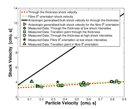
Figure 4: Anisotropic generalised bulk $U^{A}_{s}$ shock velocity, longitudinal (through the thickness) $U^{L}_{s}$ shock velocity and longitudinal (fibre $0^{o}$ orientation) $U^{F}_{s}$ shock velocity for a single wave structure of carbon fibre-epoxy composite under shock loading, where $U^{L}_{s}$ is defined by (29).

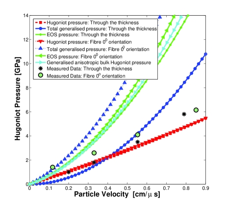
Figure 5: Comparison of the different Shock Hugoniot pressures $P^{L}_{H}$, $P^{*}_{L}$, $P^{EOS}_{L}$, $P^{F}_{H}$, $P^{*}_{F}$, $P^{EOS}_{F}$ and $P^{A}_{H}$ for a single-wave structure of the carbon-fibre epoxy composite behind the shock wave in stress-particle velocity space. The $P^{L}_{H}$, $P^{F}_{H}$ and $P^{A}_{H}$ curves are calculated from the equations $P^{L}_{H}=\rho^{A}_{0}U^{L}_{s}u_{p}$, $P^{F}_{H}=\rho^{A}_{0}U^{F}_{s}u_{p}$ and $P^{A}_{H}=\rho^{A}_{0}U^{A}_{s}u_{p}$ respectively, where $U^{A}_{s}$ is defined by (29). The $P^{*}_{L}$, $P^{EOS}_{L}$, $P^{*}_{F}$ and $P^{EOS}_{F}$ curves are defined by (12) and (13).

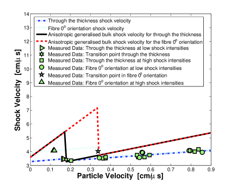
Figure 6: Anisotropic generalised bulk $U^{A}_{s}$ shock velocity, longitudinal (through the thickness) $U^{L}_{s}$ shock velocity and longitudinal (fibre $0^{o}$ orientation) $U^{F}_{s}$ shock velocity for a two-wave structure of carbon fibre-epoxy composite under shock loading, where $U^{L}_{s}$ is defined by (30).

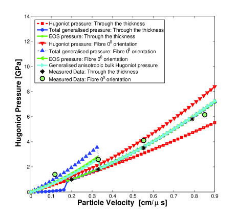
Figure 7: Comparison of the different Shock Hugoniot pressures $P^{L}_{H}$, $P^{*}_{L}$, $P^{EOS}_{L}$, $P^{F}_{H}$, $P^{*}_{F}$, $P^{EOS}_{F}$ and $P^{A}_{H}$ for a two-wave structure of the carbon-fibre epoxy composite behind the shock wave in stress-particle velocity space. The $P^{L}_{H}$, $P^{F}_{H}$ and $P^{A}_{H}$ curves are calculated from equations $P^{L}_{H}=\rho^{*}_{0}U^{L}_{s}u_{p}$, $P^{F}_{H}=\rho^{*}_{0}U^{F}_{s}u_{p}$ and $P^{A}_{H}=\rho^{*}_{0}U^{A}_{s}u_{p}$ respectively, where $U^{A}_{s}$ is defined by (30). The $P^{*}_{L}$, $P^{EOS}_{L}$, $P^{*}_{F}$ and $P^{EOS}_{F}$ curves are defined by (12) and (13).

According to the generalised decomposition (1), the stress tensor has been split into the generalised spherical component, $p^{\ast}\alpha_{ij}$, and the generalised deviatoric component, $\tilde{S}_{ij}$. The total generalised anisotropic ”pressure”, $p^{\ast}$, comprises a sum of two terms, $p^{*}=p^{EOS}+p^{\tilde{S}}$, where $p^{EOS}$ corresponds to the thermodynamic (EOS) response calculated from (14) - (15) and $p^{\tilde{S}}$ corresponds to the generalised deviatoric stress calculated using (5).

Figures (5) and (7) display $p^{*}$ and $p^{EOS}$. It can be seen that there is an increasing divergence of $p^{\ast}$ from $p^{EOS}$ due to greater particle velocities associated with an increased contribution from $p^{\tilde{S}}$. In addition, it can be seen that pressure $p^{EOS}$ for the selected CFC material is greater than the generalised total pressure, $p^{\ast}$. Further comparison of different pressures (see Figs. (5) and (7)) shows that there is an increasing divergence between the measured Hugoniot stress (HSLs) and the calculated pressures $P^{F}_{H}$, $P^{L}_{H}$, $p^{EOS}_{F}$, $p^{EOS}_{L}$, $p^{*}_{F}$ and $p^{*}_{L}$ - this corresponds to the increasing contribution from the generalised deviator of the stress tensor, $\tilde{S}^{H}_{ij}$. In addition, it is important to analyse the difference between the shock velocities in the two-wave structure at the phase transition point, these evaluated using:

$$\left[U^{L}_{s}\right]=\left(c^{AL}_{0}-c^{IL}_{0}\right)+\left(S^{AL}_{1}-S^{IL}_{1}\right)u_{p},$$ (34)

$$\left[U^{F}_{s}\right]=\left(c^{AF}_{0}-c^{IF}_{0}\right)+\left(S^{AF}_{1}-S^{IF}_{1}\right)u_{p},$$ (35)

where $\left[U^{L}_{s}\right]_{u_{p}=u^{*}_{l}}=154.935\ m/s$ for the through thickness orientation and $\left[U^{F}_{s}\right]_{u_{p}=u^{*}_{f}}=754.705\ m/s$ for the fibre $0^{o}$ orientation at the transition points $u^{*}_{l}$ and $u^{*}_{f}$ respectively. Using fitted EOS data (see Table 3), the difference between shock waves at the transition point for the through thickness orientation is smaller than that along the fibre $0^{o}$ orientation. Therefore, the material behaviour through the thickness orientation can be approximated with a single wave structure (see Figure 4), this confirmed during the examination of Hugoniot Stress Levels (HSLs) through the thickness orientation in terms of the particle velocities Lukyanov7 (33).

Finally, in Figs. (8) and (9), the effect of orientation on the Hugoniot Stress Levels (HSLs) in stress-particle velocity space is examined for single wave and two-wave structures. It can be seen from the experimental points in Figs. (8), (9) that, at lower stresses, the mixture of epoxy binder and $0^{o}$ fibres is stiffer, however, as stress increases, the experimental Hugoniots for a mixture (CFC composite) of both orientations converge. This is in agreement with the behaviour of the shock velocities shown in Fig. (9) for a two-wave structure. It is also clear from Fig. (8) that a single wave structure is not capable of predicting correctly the Hugoniot Stress Levels (HSLs) along the fibre $0^{o}$ orientation to agree with the stability requirements formulated by Bethe Bethe (30). It is important to note that there is no true prediction of the experimental data shown in figures (8) and (9) for through the thickness orientation. These experimental points (through the thickness) have been used to define the material parameters in the presented anisotropic EOS model. There is only a true prediction of the experimental data shown in figures (8) and (9) for along the fibre $0^{o}$ orientation.

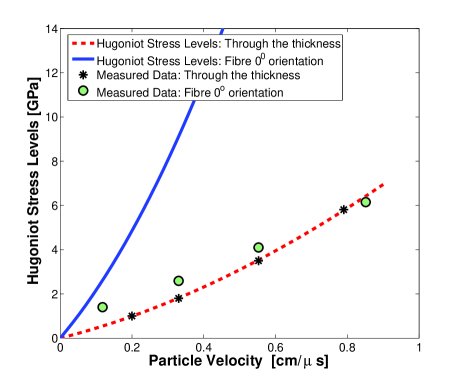
Figure 8: Hugoniot Stress Levels (HSLs) for a carbon-fibre epoxy composite behind the shock wave in the through thickness and fibre $0^{o}$ orientations in stress-particle velocity space, assuming a single wave structure. The experimental data for Hugoniot Stress Levels (HSLs) was obtained by Millett et al. MillettLukyanov (23). The dotted curve is calculated using the anisotropic EOS proposed in (31), (32) and experimental data for the through thickness orientation $U^{L}_{S}-u_{p}$. The solid curve is calculated using the anisotropic EOS proposed in (31), (32) and experimental data for the fibre $0^{o}$ orientation $U^{F}_{S}-u_{p}$.

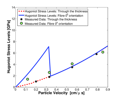
Figure 9: Hugoniot Stress Levels (HSLs) for a carbon-fibre epoxy composite behind the shock wave in the through thickness and fibre $0^{o}$ orientations in stress-particle velocity space, assuming a two-wave structure. The experimental data for Hugoniot Stress Levels (HSLs) was obtained by Millett et al. MillettLukyanov (23). The dotted curve is calculated using the anisotropic EOS proposed in (31), (32) and experimental data for the through thickness orientation $U^{L}_{S}-u_{p}$. The solid curve is calculated using the anisotropic EOS proposed in (31), (32) and experimental data for the fibre $0^{o}$ orientation $U^{F}_{S}-u_{p}$.

Figures (8), (9) show qualitatively that the anisotropy of a composite material (carbon fibre-epoxy composite) has a strong effect on the accurate extrapolation of high-pressure shock Hugoniot states to other thermodynamic states for shocked anisotropic composite (CFC) materials (e.g., a carbon-fibre epoxy composite) of any symmetry.

IV Conclusions

An anisotropic equation of state is proposed for the accurate extrapolation of high-pressure shock Hugoniot states to other thermodynamic states, for a shocked carbon-fibre epoxy composite (CFC) of any symmetry. The proposed equation of state, which uses a generalised decomposition of the stress tensor Lukyanov2 (24, 25, 26, 27, 28), represents the mathematical and physical generalisation of the Mie-Grüneisen equation of state for an isotropic material, and reduces to the latter in the limit of isotropy.

Further insights into the anisotropic CFC response under shock loading can be gained from an examination of the material EOS in terms of: shock stresses (total generalised anisotropic pressure, $p^{*}$; generalised anisotropic bulk Hugoniot pressure, $P^{A}_{H}$; pressure, $p^{EOS}$, corresponding to the thermodynamic (equation of state) response; pressure, $p^{\tilde{S}}$, corresponding to the generalised deviatoric stress), shock velocities (shock velocity in the through-thickness orientation, $U^{L}_{S}$, shock velocity in the fibre $0^{o}$ orientation, $U^{F}_{S}$, and the generalised anisotropic bulk shock velocity, $U^{A}_{s}$) and the particle velocity, $u^{p}$. Figure (6) shows linear relationships, for a two-wave structure, between the shock velocities $U^{L}_{s},U^{F}_{S},U^{A}_{S}$ and the particle velocities, $u_{p}$, over the range of measurements made during experiments. The values of $c^{AL}_{0},c^{AF}_{0},c^{AA}_{0}$ and $c^{IL}_{0},c^{IF}_{0},c^{IA}_{0}$ were determined. The values $c^{AA}_{0}$ and $c^{IA}_{0}$ (the intercept of the $U^{A}_{s}$-$u_{p}$ curve for two-wave structure) are in the interval between the first and second generalised anisotropic bulk speeds of sound Lukyanov3 (25) (for non-linear anisotropic elastic and isotropic elastic shock waves). This is a behaviour that is observed in many polymers, including epoxy resins. When $c^{AL}_{0}$, $c^{AF}_{0}$ and $c^{AA}_{0}$ are compared to the measured longitudinal sound speed $C_{L}$ (Table 1, Table 3), it can be seen that the former values are significantly greater than the latter, in the through thickness orientation. This indicates that, for highly anisotropic materials, anisotropic shock fronts (at lower particle velocity) are always supersonic with respect to the longitudinal sound speed in the least stiff direction (for example, longitudinal sound speed in the through thickness orientation). It is possible that the generalised anisotropic bulk shock velocity, $U^{A}_{s}$, depends non-linearly on particle velocity for a given anisotropic material (or composite materials), as has been shown for some isotropic polymers such as PMMA BarkerHollenbach (1) – unfortunately, the corresponding experimental data for carbon fibre materials (or other anisotropic materials) cannot be located at this time.

An analytical calculation showed that the Hugoniot Stress Levels (HSLs) for a carbon-fibre epoxy composite do not agree with the experimental data for a single wave structure methodology for the stability requirements formulated by Bethe Bethe (30). However, the material behaviour in the through-thickness orientation can be approximated by a single wave structure due to the lack of any significant discontinuity at the transition zone Lukyanov7 (33). This approximation will not take into account changes in the material elastic properties during the damage softening process. In addition, an analytical calculation showed that the Hugoniot Stress Levels (HSLs) in different directions, for a CFC composite subject to the two-wave structure (non-linear anisotropic and isotropic elastic waves), agree with experimental measurements at both low shock intensities (where the $0^{0}$ orientation was significantly stiffer than the through-thickness orientation) and at high shock intensities (where the HSLs of the two orientations converged due to the presence of damage softening), this also in agreement with the stability requirements formulated by Bethe Bethe (30).

V Acknowledgments

Author thanks Prof. V. Penjkov, Dr. B. Cox and Dr. B. Wells for many useful suggestions regarding this work. The discussions regarding the shock wave experiments on a carbon-fibre epoxy composite with Dr. J. C. F. Millett during the meetings at Cranfield University are also greatly appreciated.

References

• (1) L.M. Barker, R.E. Hollenbach, J. Appl. Phys. 43, 4669 (1972)
• (2) G.I. Kanel, J. Mech. Phys. Solids 43 (10), 1869 (1998)
• (3) G.I. Kanel, K. Baumung, H. Bluhm, V.E. Fortov, Nucl. Instr. Meth. Phys. Res. A 415, 509 (1998)
• (4) N.K. Bourne, G.S. Stevens, Rev. Sci. Instrum. 72 (4), 2214 (2001)
• (5) N.K. Bourne, Meas. Sci. & Technol. 14, 273 (2003)
• (6) L. Davison, R.A. Graham, Shock Compres. solids Phys. Rep. 55, 255 (1979)
• (7) A.V. Bushman, G.I. Kanel, A.L. Ni, V.E. Fortov, Intense dynamic Loading of Condensed Matter (Taylor and Francis, Washington, D.C., 1993)
• (8) M.A. Meyers, Dynamic Behavior of Materials (Wiley, Inc., New York, 1994)
• (9) D.J. Steinberg, Report No. UCRL-MA-106439, Lawrence Livermore National Laboratory, Livermore, CA (1991)
• (10) A.B. Kiselev, A.A. Lukyanov, Int. J. Forming Processes 5, 359 (2002)
• (11) D.P. Dandekar, C.A. Hall, L.C. Chhabildas, W.D. Reinhart, Compos. Struc. 61, 51 (2003)
• (12) D.E. Munson, R.P. May, J. Appl. Phys. 43, 962 (1972)
• (13) J.C.F. Millett, N.K. Bourne , N.R. Barnes, J. Appl. Phys. 92, 6590 (2002)
• (14) A.Z. Zhuk, G.I. Kanel, A.A. Lash, J. Phys. IV 4, 403 (1994)
• (15) W. Riedel, H. Nahme, K. Thoma, In: Furnish MD, Gupta YM, Forbes JW, editors. Shock compression of condensed matter 2003. Melville, N.Y.: AIP Press, 701 (2004)
• (16) E. Zaretsky, G. deBotton, M. Perl, Int. J. Solids Struct. 41, 569 (2004)
• (17) J.K. Chen, A. Allahdadi, T. Carney, Comp. Sci. and Techn. 57, 1268 (1997)
• (18) C.J. Hayhurst, S.J. Hiermaier, R.A. Clegg, W. Riedel, and M. Lambert, Int. J. Impact Engineering 23(1), 365 (1999)
• (19) C.E. Anderson, Jr.P.E. O’Donoghue, D. Skerhut, J. Comp. Materials 24, 1159 (1990)
• (20) C.E. Anderson, P.A. Cox, G.R. Johnson, P.J. Maudlin, Comput. Mech. 15, 201 (1994)
• (21) S.A. Bordzilovsky, S.M. Karakhanov, L.A. Merzhievsky, In: Schmidt S.C., Dandekar D.P., Forbes J.W., editors. Shock compression of condensed matter 1997. Melville, N.Y.: AIP Press, 545 (1998)
• (22) P-L Hereil, O. Allix, M. Gratton, J. Phys. IV 7, 529 (1997)
• (23) J.C.F. Millett, N.K. Bourne, Y.J.E. Meziere, R. Vignjevic, A.A. Lukyanov, Comp. Sci. and Techn. 67(15-16), 3253 (2007)
• (24) A.A. Lukyanov, Int. J. Plasticity 24, 140 (2008)
• (25) A.A. Lukyanov, Eur. Phys. J. B 64, 159 (2008)
• (26) A.A. Lukyanov, J. Appl. Mech. 76, 061012-1 (2009)
• (27) A.A. Lukyanov, ASME Proceeding IPC2006, ISBN 0-7918-3788-2 (2006)
• (28) A.A. Lukyanov, J. Pressure Vessel Technology 130, 021701-1 (2008)
• (29) A.A. Lukyanov, V.B. Penjkov, J. Appl. Math. Mech. 73 (4), (2009)
• (30) H.A. Bethe, Office of Scientific Res. and Develop. Rept. No. 545, Serial No. 237 (1942).
• (31) J.P. Poirier, Introduction to the Physics of the Earth’s Interior (Cambridge: Univ. Press, 2000)
• (32) W.J. Carter, S.P. Marsh, Report No. LA-12006-MS, Los Alamos National Laboratory, LA (1995)
• (33) A.A. Lukyanov, Mech. Advan. Mater. and Struct., Special Issue: ICCS15. Accepted (2009)