Computation- and Space-Efficient Implementation of SSA

Abstract

The computational complexity of different steps of the basic SSA is discussed. It is shown that the use of the general-purpose ‘‘blackbox’’ routines (e.g. found in packages like LAPACK) leads to huge waste of time resources since the special Hankel structure of the trajectory matrix is not taken into account.

We outline several state-of-the-art algorithms (for example, Lanczos-based truncated SVD) which can be modified to exploit the structure of the trajectory matrix. The key components here are Hankel matrix-vector multiplication and the Hankelization operator. We show that both can be computed efficiently by the means of Fast Fourier Transform.

The use of these methods yields the reduction of the worst-case computational complexity from $O(N^{3})$ to $O(kN\log{N})$, where $N$ is series length and $k$ is the number of eigentriples desired.

1 Introduction

Despite the recent growth of SSA-related techniques it seems that little attention was paid to their efficient implementations, e.g. the singular value decomposition of Hankel trajectory matrix, which is a dominating time-consuming step of the basic SSA.

In almost all SSA-related applications only a few leading eigentriples are desired, thus the use of general-purpose ‘‘blackbox’’ SVD implementations causes a huge waste of time and memory resources. This almost prevents the use of the optimum window sizes even on moderate length (say, few thousand) time series. The problem is much more severe for 2D-SSA [15] or subspace-based methods [2, 8, 13], where large window sizes are typical.

We show that proper use of state-of-art singular value decomposition algorithms can significantly reduce the amount of operations needed to compute truncated SVD suitable for SSA purposes. This is possible because the information about the leading singular triples becomes available long before the costly full decomposition.

These algorithms are usually based on Lanczos iterations or related methods. This algorithm can be modified to exploit the Hankel structure of the data matrix effectively. Thus the computational burden of SVD can be considerably reduced.

In section 2 we will outline the computational and storage complexity of the steps of the basic SSA algorithm. Section 3 contains a review of well-known results connected with the Lanczos singular value decompostion algorithm. Generic implementation issues in finite-precision arithmetics will be discussed as well. The derivation of the efficient Hankel SSA trajectory matrix-vector multiplication method will be presented in section 4. This method is a key component of the fast truncated SVD for the Hankel SSA trajectory matrices. In the section 5 we will exploit the special structure of the rank 1 Hankelization operator which allows its efficient implementation. Finally, all the implementations of the mentioned algorithms are compared in sections 6 and 7 on artificial and real data.

2 Complexity of the Basic SSA Algorithm

Let $N>2$. Denote by $F=\left(f_{1},\dots,f_{N}\right)$ a real-valued time series of length $N$. Fix the window length $L$, $1<L<N$. The Basic SSA algorithm for the decomposition of a time series consists of four steps [14]. We will consider each step separately and discuss its computational and storage complexity.

2.1 Embedding

The embedding step maps original time series to a sequence of lagged vectors. The embedding procedure forms $K=N-L+1$ lagged vectors $X_{i}\in\mathbb{R}^{L}$:

$$X_{i}=\left(f_{i},\dots,f_{i+L-1}\right)^{T},\quad 1\leqslant i\leqslant K.$$

These vectors form the $L$-trajectory (or trajectory) matrix $X$ of the series $F$:

$$X=\begin{pmatrix}f_{1}&f_{2}&\cdots&f_{K-1}&f_{K}\\ f_{2}&f_{3}&\cdots&f_{K}&f_{K+1}\\ \vdots&\vdots&&\vdots&\vdots\\ f_{L}&f_{L+1}&\cdots&f_{N-1}&f_{N}\end{pmatrix}.$$

Note that this matrix has equal values along the antidiagonals, thus it is a Hankel matrix. The computational complexity of this step is negligible: it consists of simple data movement which is usually considered a cheap procedure. However, if the matrix is stored as-is, then this step obviously has storage complexity of $O(LK)$ with the worst case being $O(N^{2})$ when $K\sim L\sim N/2$.

2.2 Singular Value Decomposition

This step performs the singular value decomposition of the $L\times K$ trajectory matrix $X$. Without loss of generality we will assume that $L\leqslant K$. Then the SVD can be written as

$$X=U^{T}\Sigma V,$$

where $U=\left(u_{1},\dots,u_{L}\right)$ is a $L\times L$ orthogonal matrix, $V=\left(v_{1},\dots,v_{K}\right)$ is a $K\times K$ orthogonal matrix, and $\Sigma$ is a $L\times K$ diagonal matrix with nonnegative real diagonal entries $\Sigma_{ii}=\sigma_{i}$, for $i=1,\dots,L$. The vectors $u_{i}$ are called left singular vectors, the $v_{i}$ are the right singular vectors, and the $\sigma_{i}$ are the singular values. We will label the singular values in descending order: $\sigma_{1}\geqslant\sigma_{2}\geqslant\cdots\geqslant\sigma_{L}$. Note that the singular value decomposition of $X$ can be represented in the form

$$X=X_{1}+\cdots+X_{L},$$

where $X_{i}=\sigma_{i}u_{i}v_{i}^{T}$. The matrices $X_{i}$ have rank $1$, therefore we will call them elementary matrices. The triple $\left(\sigma_{i},u_{i},v_{i}\right)$ will be called a singular triple.

Usually the SVD is computed by means of Golub and Reinsh algorithm [12] which requires $O(L^{2}K+LK^{2}+K^{3})$ multiplications having the worst computational complexity of $O(N^{3})$ when $K\sim L\sim N/2$. Note that all the data must be processed at once and SVDs even of moderate length time series (say, when $N>5000$) are essentially unfeasible.

2.3 Grouping

The grouping procedure partitions the set of indices $\left\{1,\dots,L\right\}$ into $m$ disjoint sets $I_{1},\dots,I_{m}$. For the index set $I=\left\{i_{1},\dots,i_{p}\right\}$ one can define the resultant matrix $X_{I}=X_{i_{1}}+\cdots+X_{i_{p}}$. Such matrices are computed for $I=I_{1},\dots,I_{m}$ and we obtain the decomposition

$$X=X_{I_{1}}+\cdots+X_{I_{m}}.$$

For the sake of simplicity we will assume that $m=L$ and each $I_{j}=\left\{j\right\}$ later on. The computation of each elementary matrix $X_{j}$ costs $O(LK)$ multiplications and $O(LK)$ storage yielding overall computation complexity of $O(L^{2}K)$ and $O(L^{2}K)$ for storage. Again the worst case is achieved at $L\sim K\sim N/2$ with the value $O(N^{3})$ for both computation and storage.

2.4 Diagonal Averaging (Hankelization)

This is the last step of the Basic SSA algorithm transforming each grouped matrix $X_{I_{j}}$ into a new time series of length $N$. This is performed by means of diagonal averaging procedure (or Hankelization). It transforms an arbitrary $L\times K$ matrix $Y$ to the series $g_{1},\dots,g_{N}$ by the formula:

$$g_{k}=\begin{cases}\frac{1}{k}\sum_{j=1}^{k}{y_{j,k-j+1}},&\quad 1\leqslant k\leqslant L,\\ \frac{1}{L}\sum_{j=1}^{L}{y_{j,k-j+1}},&\quad L<k<K,\\ \frac{1}{N-k+1}\sum_{j=k-K+1}^{L}{y_{j,k-j+1}},&\quad K\leqslant k\leqslant N.\end{cases}$$

Note that these two steps are usually combined. One just forms the elementary matrices one by one and immediately applies the Hankelization operator. This trick reduces the storage requirements considerably.

$O(N)$ multiplications and $O(LK)$ additions are required for performing the diagonal averaging of one elementary matrix. Summing these values for $L$ elementary matrices we obtain the overall computation complexity for this step being $O(L^{2}K)$ additions and $O(NL)$ multiplications. The worst case complexity will be then $O(N^{3})$ additions and $O(N^{2})$ multiplications

Summing the complexity values alltogether for all four steps we obtain the worst case computational complexity to be $O(N^{3})$. The worst case occurs exactly when window length $L$ equals $N/2$ (the optimal window length for asymptotic separability [14]).

3 Truncated Singular Value Decomposition

The typical approach to the problem of computating the singular triples $\left(\sigma_{i},u_{i},v_{i}\right)$ of $A$ is to use the Schur decomposition of some matrices related to $A$, namely

1. the cross product matrices $AA^{T}$, $A^{T}A$, or

2. the cyclic matrix $C=\left(\begin{smallmatrix}0&A\\ A^{T}&0\end{smallmatrix}\right)$.

One can prove the following theorem (see, e.g. [11, 19]):

Theorem 1

Let $A$ be an $L\times K$ matrix and assume without loss of generality that $K\geqslant L$. Let the singular value decomposition of $A$ be

$$U^{T}AV=\operatorname*{\mathrm{diag}\,}\left(\sigma_{1},\dots,\sigma_{L}\right).$$

Then

$$V^{T}\left(A^{T}A\right)V = \operatorname*{\mathrm{diag}\,}(\sigma_{1}^{2},\dots,\sigma_{L}^{2},\underbrace{0,\dots,0}_{K-L}),$$

$$U^{T}\left(AA^{T}\right)U = \operatorname*{\mathrm{diag}\,}(\sigma_{1}^{2},\dots,\sigma_{L}^{2}).$$

Moreover, if $V$ is partitioned as

$$V=\left(V_{1},V_{2}\right),\quad V_{1}\in\mathbb{R}^{K\times L},V_{2}\in\mathbb{R}^{K\times(K-L)},$$

then the orthonormal columns of the $(L+K)\times(L+K)$ matrix

$$Y=\frac{1}{\sqrt{2}}\begin{pmatrix}U&-U&0\\ V_{1}&V_{1}&\sqrt{2}V_{2}\end{pmatrix}$$

form an eigenvector basis for the cyclic matrix $C$ and

$$Y^{T}CY=\operatorname*{\mathrm{diag}\,}(\sigma_{1},\dots,\sigma_{L},-\sigma_{1},\dots,-\sigma_{L},\underbrace{0,\dots,0}_{K-L}).$$

The theorem tells us that we can obtain the singular values and vectors of $A$ by computing the eigenvalues and corresponding eigenvectors of one of the symmetric matrices. This fact forms the basis of any $SVD$ algorithm.

In order to find all eigenvalues and eigenvectors of the real symmetric matrix one usually turns it into a similar tridiagonal matrix by the means of orthogonal transformations (Householder rotations or alternatively via Lanczos recurrenses). Then, for example, another series of orthogonal transformations can be applied to the latter tridiagonal matrix which converges to a diagonal matrix [11].

Such approach, which in its original form is due to Golub and Reinsh [12] and is used in e.g. LAPACK [1], computes the SVD by implicitly applying the QR algorithm to the symmetric eigenvalue problem for $A^{T}A$.

For large and sparse matrices the Golub-Reinsh algorithm is impractical. The algorithm itself starts out by applying a series of transformations directly to matrix $A$ to reduce it to the special bidiagonal form. Therefore it requires the matrix to be stored explicitlly, which may be impossible simply due to its size. Moreover, it may be difficult to take advantage of any structure (e.g. Hankel in SSA case) or sparsity in $A$ since it is quickly destroyed by the transformations applied to the matrix. The same argument applies to SVD computation via the Jacobi algorithm.

Bidiagonalization was proposed by Golub and Kahan [10] as a way of tridiagonalizing the cross product matrix without forming it explicitly. The method yields the decomposition

$$A=P^{T}BQ,$$

where $P$ and $Q$ are orthogonal matrices and $B$ is an $L\times K$ lower bidiagonal matrix. Here $BB^{T}$ is similar to $AA^{T}$. Additionally, there are well-known SVD algorithms for real bidiagonal matrices, for example, the QR method [11], divide-and-conquer [16], and twisted [7] methods.

The structure of our exposition follows [19].

3.1 Lanczos Bidiagonalization

For a rectangular $L\times K$ matrix $A$ the Lanczos bidiagonalization computes a sequence of left Lanczos vectors $u_{j}\in\mathbb{R}^{L}$ and right Lanczos vectors $v_{j}\in\mathbb{R}^{K}$ and scalars $\alpha_{j}$ and $\beta_{j}$, $j=1,\dots,k$ as follows:

Choose a starting vector $p_{0}\in\mathbb{R}^{L}$

$\beta_{1}\longleftarrow\left\|p_{0}\right\|_{2}$, $u_{1}\longleftarrow p_{0}/\beta_{1}$, $v_{0}\longleftarrow 0$

for $j\leftarrow 1$ to $k$ do $r_{j}\longleftarrow A^{T}u_{j}-\beta_{j}v_{j-1}$

$\alpha_{j}\longleftarrow\left\|r_{j}\right\|_{2}$,   $v_{j}\longleftarrow r_{j}/\alpha_{j}$

$p_{j}\longleftarrow Av_{j}-\alpha_{j}u_{j}$

$\beta_{j+1}\longleftarrow\left\|p_{j}\right\|_{2}$,   $u_{j+1}\longleftarrow p_{j}/\beta_{j+1}$

end

Algorithm 1 Golub-Kahan-Lanczos Bidiagonalization

Later on we will refer to one iteration of the for loop at line 1 as a Lanczos step (or iteration). After $k$ steps we will have the lower bidiagonal matrix

$$B_{k}=\begin{pmatrix}\alpha_{1}&&&\\ \beta_{2}&\alpha_{2}&&\\ &\beta_{3}&\ddots&\\ &&\ddots&\alpha_{k}\\ &&&\beta_{k+1}\end{pmatrix}.$$

If all the computations performed are exact, then the Lanczos vectors will be orthornomal:

$$U_{k+1}=\left(u_{1},\dots,u_{k+1}\right)\in\mathbb{R}^{L\times(k+1)},\quad U_{k+1}^{T}U_{k+1}=I_{k+1},$$

and

$$V_{k+1}=\left(v_{1},\dots,v_{k+1}\right)\in\mathbb{R}^{K\times(k+1)},\quad V_{k+1}^{T}V_{k+1}=I_{k+1},$$

where $I_{k}$ is $k\times k$ identity matrix. By construction, the columns of $U_{k+1}$ and $V_{k+1}$ satisfy the recurrences

$$\alpha_{j}v_{j} = A^{T}u_{j}-\beta_{j}v_{j-1},$$

$$\beta_{j+1}u_{j+1} = Av_{j}-\alpha_{j}u_{j},$$

and can be written in the compact form as follows:

$$AV_{k} = U_{k+1}B_{k},$$ (1)

$$A^{T}U_{k+1} = V_{k}B_{k}^{T}+\alpha_{k+1}v_{k+1}e_{k+1}^{T}.$$ (2)

Also, the first equiality can be rewritten as

$$U^{T}_{k+1}AV_{k}=B_{k},$$

explaining the notion of left and right Lanczos vectors. Moreover, $u_{k}\in\mathcal{K}_{k}\left(AA^{T},u_{1}\right)$, $v_{k}\in\mathcal{K}_{k}\left(A^{T}A,v_{1}\right)$, where

$$\mathcal{K}_{k}\left(AA^{T},u_{1}\right)=\left\{u_{1},AA^{T}u_{1},\dots,\left(AA^{T}\right)^{k}u_{1}\right\},$$ (3)

$$\mathcal{K}_{k}\left(A^{T}A,v_{1}\right)=\left\{v_{1},A^{T}Av_{1},\dots,\left(A^{T}A\right)^{k}v_{1}\right\},$$ (4)

and therefore $u_{1},u_{2},\dots,u_{k}$ and $v_{1},v_{2},\dots,v_{k}$ form an orthogonal basis for these two Krylov subspaces.

6

6

6

6

6

6

3.2 Lanczos Bidiagonalization in Inexact Arithmetics

When the Lanczos bidiagonalization is carried out in finite precision arithmetics the Lanczos recurrence becomes

$$\alpha_{j}v_{j} = A^{T}u_{j}-\beta_{j}v_{j-1}+f_{j},$$

$$\beta_{j+1}u_{j+1} = Av_{j}-\alpha_{j}u_{j}+g_{j},$$

where $f_{j}\in\mathbb{R}^{K}$, $g_{j}\in\mathbb{R}^{L}$ are error vectors accounting for the rounding errors at the $j$-th step. Usually, the rounding terms are small, thus after $k$ steps the equations (1), (2) still hold to almost machine accuracy. In contrast, the orthogonality among left and right Lanczos vectors is lost.

However, the Lanzos algorithm possesses a remarkable feature that the accuracy of the converged Ritz values is not affected by the loss of orthogonality, but while the largest singular values of $B_{k}$ are still accurate approximations to the largest singular values of $A$, the spectrum of $B_{k}$ will in addition contain false multiple copies of converged Ritz values (this happens even if the corresponding true singular values of $A$ are isolated). Moreover, spurious singular values (‘‘ghosts’’) periodically appear between the already converged Ritz values (see, e.g. [19] for illustration).

There are two different approaches with respect to what should be done to obtain a robust method in finite arithmetics.

3.2.1 Lanczos Bidiagonalization with no orthogonalization

One approach is to apply the simple Lanczos process ‘‘as-is’’ and subsequently use some criterion to detect and remove spurious singular values.

The advantage of this method is that it completely avoids any extra work connected with the reorthogonalization, and the storage requirements are very low since only few of the latest Lanczos vectors have to be remembered. The disadvantage is that many iterations are wasted on simply generating multiple copies of the large values [23]. The number of extra iterations required compared to that when executing the Lanczos process in exact arithmetics can be very large: up to six times the original number as reported in [24]. Another disdvantage is that the criterion mentioned above can be rather difficult to implement, since it depends on the correct choice of different thresholds and knobs.

3.2.2 Lanczos Bidiagonalization using reorthogonalization

A different way to deal with loss of orthogonalizy among Lanczos vectors is to apply some reorthogonalization scheme. The simplest one is so-callled full reorthogonalization (FRO) where each new Lanczos vector $u_{j+1}$ (or $v_{j+1}$) is orthogonalized against all the Lanczos vectors generated so far using, e.g., the modified Gram-Schmidt algorithm.

This approach is usually too expensive, since for the large problem the running time needed for reorthogonalization quickly dominate the execution time unless the necessary number of iterations $k$ is very small compared to the dimensions of the problem (see section 3.3 for full analysis of the complexity). The storage requirements of FRO might also be a limiting factor since all the generated Lanczos vectors need to be saved.

A number of different schemes for reducing the work associated with keeping the Lanczos vectors orthogonal were developed (see [3] for extensive review). The main idea is to estimate the level of orthogonality among the Lanczos vectors and perform the orthogonalization only when necessary.

For example, the so-called partial reorthogonalization scheme (PRO) described in [27, 26, 19] uses the fact that the level of orthogonality among the Lanczos vectors satisfies some recurrence relation which can be derived from the recurrence used to generate the vectors themselves.

3.3 The Complexity of the Lanczos Bidiagonalization

The computational complexity of the Lanczos bidiagonalization is determined by the two matrix-vector multiplications, thus the overall complexity of $k$ Lanczos iterations in exact arithmetics is $O(kLK)$ multiplications.

The computational costs increase when one deals with the lost of orthogonality due to the inexact computations. For FRO scheme the additional $O(k^{2}(L+K))$ operations required for the orthogonalization quickly dominate the execution time, unless the necessary number of iterations $k$ is very small compared to the dimension of the problem. The storage requirements of FRO may also be a limiting factor since all the generated Lanczos vectors need to be saved.

In general, there is no way to determine in advance how many steps will be needed to provide the singular values of interest within a specified accuracy. Usually the number of steps is determined by the distribution of the singular numbers and the choice of the starting vector $p_{0}$. In the case when the singular values form a cluster the convergence will not occur until $k$, the number of iterations, gets very large. In such situation the method will also suffer from increased storage requirements: it is easy to see that they are $O(k(L+K))$.

These problems can be usually solved via limiting the dimension of the Krylov subspaces (3), (4) and using restarting schemes: restarting the iterations after a number of steps by replacing the starting vector with some ‘‘improved’’ starting vector (ideally, we would like $p_{0}$ to be a linear combination of the right singular vectors of $A$ associated with the desired singular values). Thus, if we limit the dimension of the Krylov subspaces to $d$ the storage complexity drops to $O(d(L+K))$ (surely the number of desired singular triples should be greater than $d$). See [3] for the review of the restarting schemes proposed so far and introduction to the thick-restarted Lanczos bidiagonalization algorithm. In the papers [30, 31] different strategies of choosing the best dimension $d$ of Krylov subspaces are discussed.

If the matrix being decomposed is sparse or structured (for example, Hankel in Basic SSA case or Hankel with Hankel blocks for 2D-SSA) then the computational complexity of the bidiagonalization can be significantly reduced given that the efficient matrix-vector multiplication routine is available.

4 Efficient Matrix-Vector Multiplication for Hankel Matrices

In this section we will present efficient matrix-vector multiplication algorithm for Hankel SSA trajectory matrix. By means of the fast Fourier transform the cost of the multiplication drops from ordinary $O(LK)$ multiplications to $O\left((L+K)\log(L+K)\right)$. The idea of using the FFT for computing a Hankel matrix-vector product is nothing new: it was probably first described by Bluestein in 1968 (see [28]). A later references are [21, 5].

This approach reduces the computational complexity of the singular value decomposition of Hankel matrices from $O\left(kLK+k^{2}(L+K)\right)$ to $O\left(k(L+K)\log(L+K)+k^{2}(L+K)\right)$. The complexity of the worst case when $K\sim L\sim N/2$ drops significantly from $O\left(kN^{2}+k^{2}N\right)$ to $O\left(kN\log{N}+k^{2}N\right)$​​.

Also the discribed algorithms provide an efficient way to store the Hankel SSA trajectory matrix reducing the storage requirements from $O(LK)$ to $O(L+K)$.

4.1 Matrix Representation of Discrete Fourier Transform and Circulant Matrices

The 1-d discrete Fourier transform (DFT) of a (complex) vector $\left(f_{k}\right)_{k=0}^{N-1}$ is defined by:

$$\hat{f}_{l}=\sum_{k=0}^{N}{e^{-2\pi ikl/N}f_{k}},\quad k=0,\dots,N-1.$$

Denote by $\omega$ the primitive $N$-root of unity, $\omega=e^{-2\pi i/N}$. Introduce the DFT matrix $\mathbb{F}_{N}$:

$$\mathbb{F}_{N}=\begin{pmatrix}1&1&\cdots&1\\ 1&\omega^{1}&\cdots&\omega^{N-1}\\ 1&\omega^{2}&\cdots&\omega^{2(N-1)}\\ \vdots&\vdots&\vdots&\vdots\\ 1&\omega^{N-1}&\cdots&\omega^{(N-1)(N-1)}\end{pmatrix}.$$

Then the 1-d DFT can be written in matrix form: $\hat{f}=\mathbb{F}_{N}f$. The inverse of the DFT matrix is given by

$$\mathbb{F}_{N}^{-1}=\frac{1}{N}\mathbb{F}_{N}^{*},$$

where $\mathbb{F}_{N}^{*}$ is the adjoint (conjugate transpose) of DFT matrix $\mathbb{F}_{N}$. Thus, the inverse 1-d discrete Fourier transform (IDFT) is given by

$$f_{k}=\frac{1}{N}\sum_{l=0}^{N-1}{e^{2\pi ikl/N}\hat{f}_{l}},\quad k=0,\dots,N-1.$$

The fast Fourier transform is an efficient algorithm to compute the DFT (and IDFT) in $O(N\log{N})$ complex multiplications instead of $N^{2}$ complex multiplications in direct implementation of the DFT [20, 9].

Definition 1

An $N\times N$ matrix $C$ of the form

$$C=\begin{pmatrix}c_{1}&c_{N}&c_{N-1}&\cdots&c_{3}&c_{2}\\ c_{2}&c_{1}&c_{N}&\cdots&c_{4}&c_{3}\\ \vdots&\vdots&\vdots&&\vdots&\vdots\\ c_{N-1}&c_{N-2}&c_{N-3}&\cdots&c_{1}&c_{N}\\ c_{N}&c_{N-1}&c_{N-2}&\cdots&c_{2}&c_{1}\end{pmatrix}$$

is called a circulant matrix.

A circulant matrix is fully specified by its first column $c=\left(c_{1},c_{2},\dots,c_{N}\right)^{T}$ The remaining columns of $C$ are each cyclic permutations of the vector $c$ with offset equal to the column index. The last row of $C$ is the vector $c$ in reverse order, and the remaining rows are each cyclic permutations of the last row.

The eigenvectors of a circulant matrix of a given size are the columns of the DFT matrix of the same size. Thus a circulant matrix is diagonalized by the DFT matrix:

$$C=\mathbb{F}_{N}^{-1}\operatorname*{\mathrm{diag}\,}(\mathbb{F}_{N}c)\mathbb{F}_{N},$$

so the eigenvalues of $C$ are given by the product $\mathbb{F}_{N}c$.

This factorization can be used to perform efficient matrix-vector multiplication. Let $v\in\mathbb{R}^{N}$ and $C$ be an $N\times N$ circulant matrix. Then

$$Cv=\mathbb{F}_{N}^{-1}\operatorname*{\mathrm{diag}\,}(\mathbb{F}_{N}c)\mathbb{F}_{N}v=\mathbb{F}_{N}^{-1}\left(\mathbb{F}_{N}c\odot\mathbb{F}_{N}v\right),$$

where $\odot$ denotes the element-wise vector multiplication. This can be computed efficiently using the FFT by first computing the two DFTs, $\mathbb{F}_{N}c$ and $\mathbb{F}_{N}v$, and then computing the IDFT $\mathbb{F}_{N}^{-1}\left(\mathbb{F}_{N}c\odot\mathbb{F}_{N}v\right)$. If the matrix-vector multiplication is performed repeatedly with the same circulant matrix and different vectors, then surely the DFT $\mathbb{F}_{N}c$ needs to be computed only once.

In this way the overall computational complexity of matrix-vector product for the circulant matrices drops from $O(N^{2})$ to $O(N\log{N})$.

4.2 Toeplitz and Hankel Matrices

Definition 2

A $L\times K$ matrix of the form

$$T=\begin{pmatrix}t_{K}&t_{K-1}&\cdots&t_{2}&t_{1}\\ t_{K+1}&t_{K}&\cdots&t_{3}&t_{2}\\ \vdots&\vdots&&\vdots&\vdots\\ t_{K+L-1}&t_{K+L-2}&\cdots&t_{L+1}&t_{L}\end{pmatrix}$$

is called a (non-symmetric) Toeplitz matrix.

A Toeplitz matrix is completely determined by its last column and last row, and thus depends on $K+L-1$ parameters. The entries of $T$ are constant down the diagonals parallel to the main diagonal.

Given an algorithm for the fast matrix-vector product for circulant matrices, it is easy to see the algorithm for a Toeplitz matrix, since a Toeplitz matrix can be embedded into a circulant matrix $C_{K+L-1}$ of size $K+L-1$ with the first column equals to $\left(t_{K},t_{K+1},\dots,t_{K+L-1},t_{1},t_{2},\dots,t_{K-1}\right)^{T}$:

$$C_{K+L-1}=\begin{pmatrix}t_{K}&\cdots&t_{1}&t_{K+L-1}&\cdots&t_{K+1}\\ t_{K+1}&\cdots&t_{2}&t_{1}&\cdots&t_{K+2}\\ t_{K+2}&\cdots&t_{3}&t_{2}&\cdots&t_{K+3}\\ \vdots&&\vdots&\vdots&&\vdots\\ t_{K+L-1}&\cdots&t_{L}&t_{L-1}&\cdots&t_{1}\\ t_{1}&\cdots&t_{L+1}&t_{L}&\cdots&t_{2}\\ t_{2}&\cdots&t_{L+2}&t_{L+1}&\cdots&t_{3}\\ \vdots&&\vdots&\vdots&&\vdots\\ t_{K-1}&\cdots&t_{K+L-1}&t_{K+L-2}&\cdots&t_{K}\\ \end{pmatrix},$$ (5)

where the leading $L\times K$ principal submatrix is $T$. This technique of embedding a Toeplitz matrix in a larger circulant matrix to achieve fast computation is widely used in preconditioning methods [6].

Using this embeddings, the Toeplitz matrix-vector product $Tv$ can be represented as follows:

$$C_{K+L-1}\begin{pmatrix}v\\ \mathbf{0}_{L-1}\end{pmatrix}=\begin{pmatrix}Tv\\ *\end{pmatrix},$$ (6)

and can be computed efficiently in $O\left((K+L)\log(K+L)\right)$ time and $O(K+L)$ memory using the FFT as described previously.

Recall that an $L\times K$ matrix of form

$$H=\begin{pmatrix}h_{1}&h_{2}&\cdots&h_{K-1}&h_{K}\\ h_{2}&h_{3}&\cdots&h_{K}&h_{K+1}\\ \vdots&\vdots&&\vdots&\vdots\\ h_{L}&h_{L+1}&\cdots&h_{K+L-2}&h_{K+L-1}\end{pmatrix}$$

is called Hankel matrix.

A Hankel matrix is completely determined by its first column and last row, and thus depends on $K+L-1$ parameters. The entries of $H$ are constant along the antidiagonals. One can easily convert Hankel matrix into a Toeplitz one by reversing its columns. Indeed, define

$$P=\begin{pmatrix}0&0&\cdots&0&1\\ 0&0&\cdots&1&0\\ \vdots&\vdots&&\vdots&\vdots\\ 0&1&\cdots&0&0\\ 1&0&\cdots&0&0\end{pmatrix}$$

the backward identity permutation matrix. Then $HP$ is a Toeplitz matrix for any Hankel matrix $H$, and $TP$ is a Hankel matrix for any Toeplitz matrix $T$. Note that $P=P^{T}=P^{-1}$ as well. Now for the product $Hv$ of Hankel matrix $H$ and vector $v$ we have

$$Hv=HPPv=\left(HP\right)Pv=Tw,$$

where $T$ is Toeplitz matrix and vector $w$ is obtained as vector $v$ with entries in reversed order. The product $Tw$ can be computed using circulant embedding procedure as described in (6).

4.3 Hankel SSA Trajectory Matrices

Now we are ready to exploit the connection between the time series $F=\left(f_{j}\right)_{j=1}^{N}$ under decomposition and corresponding trajectory Hankel matrix to derive the matrix-vector multiplication algorithm in terms of the series itself. In this way we will effectively skip the embedding step of the SSA algorithm and reduce the computational and storage complexity.

The entries of the trajectory matrix of the series are $h_{j}=f_{j},\,j=1,\dots,N$. The entries of Toeplitz matrix $T=HP$ are $t_{j}=h_{j}=f_{j}$, $j=1,\dots,N$. The corresponding first column of the embedding circulant matrix (5) is

$$c_{j}=\begin{cases}t_{N-L+j}=f_{N-L+j},&\quad 1\leqslant j\leqslant L;\\ t_{j-L+1}=f_{j-L+1}&\quad L<j\leqslant N,\end{cases}$$

and we end with the following algorithm for matrix-vector multiplication for trajectory matrix:

Input: Time series $F=\left(f_{j}\right)_{j=1}^{N}$, window length $L$, vector $v$ of length $N-L+1$.

Output: $p=Xv$, where $X$ is a trajectory matrix for $F$ given window length $L$.

$c\longleftarrow\left(f_{N-L+1},\dots,f_{N},f_{1},\dots,f_{N-L}\right)^{T}$

$\hat{c}\longleftarrow FFT_{N}(c)$

$w\longleftarrow\left(v_{N-L+1},\dots,v_{1},0,\dots,0\right)^{T}$

$\hat{w}\longleftarrow FFT_{N}(w)$

$p^{\prime}\longleftarrow IFFT_{N}(\hat{w}\odot\hat{c})$

$p\longleftarrow\left(p^{\prime}_{1},\dots,p^{\prime}_{L}\right)^{T}$

Algorithm 2 Matrix-Vector Multiplication for SSA Trajectory Matrix

where $(\hat{w}\odot\hat{c})$ denotes element-wise vector multiplication.

5

5

5

5

5

If the matrix-vector multiplication $Xv$ is performed repeatedly with the same matrix $X$ and different vectors $v$ then steps 2, 2 should be performed only once at the beginning and the resulting vector $\hat{c}$ should be reused later on.

The overall computational complexity of the matrix-vector multiplication is $O(N\log{N})$. Memory space of size $O(N)$ is required to store precomputed vector $\hat{c}$.

Note that the matrix-vector multiplication of the transposed trajectory matrix $X^{T}$ can be performed using the same vector $\hat{c}$. Indeed, the bottom-right $K\times L$ submatrix of circulant matrix (5) contains the Toeplitz matrix $X^{T}P$ and we can easily modify algorithm 2 as follows:

Input: Time series $F=\left(f_{j}\right)_{j=1}^{N}$, window length $L$, vector $v$ of length $L$.

Output: $p=X^{T}v$, where $X$ is a trajectory matrix for $F$ given window length $L$.

$c\longleftarrow\left(f_{N-L+1},\dots,f_{N},f_{1},\dots,f_{N-L}\right)^{T}$

$\hat{c}\longleftarrow FFT_{N}(c)$  

$w\longleftarrow\left(0,\dots,0,v_{L},\dots,v_{1}\right)^{T}$

$\hat{w}\longleftarrow FFT_{N}(w)$

$p^{\prime}\longleftarrow IFFT_{N}(\hat{w}\odot\hat{c})$

$p\longleftarrow\left(p^{\prime}_{L-1},\dots,p^{\prime}_{N}\right)^{T}$

Algorithm 3 Matrix-Vector Multiplication for transpose of SSA Trajectory Matrix

5

5

5

5

5

5 Efficient Rank 1 Hankelization

Let us recall the diagonal averaging procedure as described in 2.4 which transforms an arbitrary $L\times K$ matrix $Y$ into a Hankel one and therefore into a series $g_{k}$, $k=1,\dots,N$.

$$g_{k}=\begin{cases}\frac{1}{k}\sum_{j=1}^{k}{y_{j,k-j+1}},&\quad 1\leqslant k\leqslant L,\\ \frac{1}{L}\sum_{j=1}^{L}{y_{j,k-j+1}},&\quad L<k<K,\\ \frac{1}{N-k+1}\sum_{j=k-K+1}^{L}{y_{j,k-j+1}},&\quad K\leqslant k\leqslant N.\end{cases}$$ (7)

Without loss of generality we will consider only rank 1 hankelization when matrix $Y$ is elementary and can be represented as $Y=\sigma uv^{T}$ with vectors $u$ and $v$ of length $L$ and $K$ correspondingly. Then equation (7) becomes

$$g_{k}=\begin{cases}\frac{\sigma}{k}\sum_{j=1}^{k}{u_{j}v_{k-j+1}},&\quad 1\leqslant k\leqslant L,\\ \frac{\sigma}{L}\sum_{j=1}^{L}{u_{j}v_{k-j+1}},&\quad L<k<K,\\ \frac{\sigma}{N-k+1}\sum_{j=k-K+1}^{L}{u_{j}v_{k-j+1}},&\quad K\leqslant k\leqslant N.\end{cases}$$ (8)

This gives a hint how the diagonal averaging can be efficiently computed.

Indeed, consider the infinite series $u^{\prime}_{n}$, $n\in\mathbb{Z}$ such that $u^{\prime}_{n}=u_{n}$ when $1\leqslant n\leqslant L$ and $0$ otherwise. The series $v^{\prime}_{n}$ are defined in the same way, so $v^{\prime}_{n}=v_{n}$ when $1\leqslant n\leqslant K$ and $0$ otherwise. The linear convolution $u^{\prime}_{n}*v^{\prime}_{n}$ of $u^{\prime}_{n}$ and $v^{\prime}_{n}$ can be written as follows:

$$\left(u^{\prime}_{n}*v^{\prime}_{n}\right)_{k}=\sum_{j=-\infty}^{+\infty}{u^{\prime}_{j}v^{\prime}_{k-j+1}}=\sum_{j=1}^{L}{u^{\prime}_{j}v^{\prime}_{k-j+1}}=\\ =\begin{cases}\sum_{j=1}^{k}{u_{j}v_{k-j+1}},&\quad 1\leqslant k\leqslant L,\\ \sum_{j=1}^{L}{u_{j}v_{k-j+1}},&\quad L<k<K,\\ \sum_{j=k-K+1}^{L}{u_{j}v_{k-j+1}},&\quad K\leqslant k\leqslant N.\end{cases}$$ (9)

Comparing the equations (7) and (9) we deduce that

$$g_{k}=c_{k}\left(u^{\prime}_{n}*v^{\prime}_{n}\right)_{k},$$

where the constants $c_{k}$ are known in advance.

The linear convolution $u*v$ can be defined in terms of the circular convolution, as follows. Pad the vectors $u$ and $v$ with the zeroes up to length $L+K-1$. Then the linear convolution of the original vectors $u$ and $v$ is the same as the circular convolution of the extended series of length $L+K-1$, namely

$$\left(u\ast v\right)_{k}=\sum_{j=1}^{L+K-1}{u_{j}v_{k-j+1}},$$

where $k-j+1$ is evaluated $\mathrm{mod}\,(L+K-1)$. The resulting circular convolution can be calculated effeciently via the FFT [4]:

$$\left(u\ast v\right)_{k}=IFFT_{N}\left(FFT_{N}(u^{\prime})\odot FFT_{N}(v^{\prime})\right).$$

Here $N=L+K-1$, and $u^{\prime}$, $v^{\prime}$ denote the zero-padded vectors $u$ and $v$ correspondingly.

And we end with the following algorithm for the hankelization via convolution:

Input: Vector $u$ of length $L$, vector $v$ of length $K$, singular value $\sigma$.

Output: Time series $G=\left(g_{j}\right)_{j=1}^{N}$ corresponding to the matrix $Y=\sigma uv^{T}$ after hankelization.

$u^{\prime}\longleftarrow\left(u_{1},\dots,u_{L},0,\dots,0\right)^{T}\in\mathbb{R}^{N}$

$\hat{u}\longleftarrow FFT_{N}(u^{\prime})$

$v^{\prime}\longleftarrow\left(v_{1},\dots,v_{K},0,\dots,0\right)^{T}\in\mathbb{R}^{N}$

$\hat{v}\longleftarrow FFT_{N}(v^{\prime})$

$g^{\prime}\longleftarrow IFFT_{N}(\hat{v}\odot\hat{u})$

$w\longleftarrow\left(1,\dots,L,L,\dots,L,L,\dots,1\right)\in\mathbb{R}^{N}$

$g\longleftarrow\sigma\left(w\odot g^{\prime}\right)$

Algorithm 4 Rank 1 Hankelization via Linear Convolution

The computational complexity of this algorithm is $O(N\log{N})$ multiplications versus $O(LK)$ for naïve direct approach. Basically this means that the worst case complexity of the diagonal averaging drops from $O(N^{2})$ to $O(N\log{N})$.

6

6

6

6

6

6

6 Implementation Comparison

The algorithms presented in this paper have much better asymptotic complexity than standard ones, but obviously might have much bigger overhead and thus would not be suitable for the real-world problems unless series length and/or window length becomes really big.

The mentioned algorithms were implemented by the means of the Rssa package for the R system for statistical computing [25]. All the comparions were carried out on the 4 core AMD Opteron 2210 workstation running Linux. Where possible we tend to use state-of-the-art implementations of various computational algorithms (e.g. highly optimized ATLAS [29] and ACML implementations of BLAS and LAPACK routines). We used R version 2.8.0 throughout the tests.

We will compare the performance of such key components of the fast SSA implementation as rank 1 diagonal averaging and the Hankel matrix-vector multiplication. The performance of the methods which use the ‘‘full’’ SSA, namely the series bootstrap confidence interval construction and series structure change detection, will be considered as well.

6.1 Fast Hankel Matrix-Vector Product

Fast Hankel matrix-vector multiplication is the key component for the Lanczos bidiagonalization. The algorithm outlined in the section 4.3 was implemented in two different ways: one using the core R FFT implementation and another one using FFT from FFTW library [9]. We selected window size equal to the half of the series length since this corresponds to the worst case both in terms of computational and storage complexity. All initialization times (for example, Hankel matrix construction or circulant precomputation times) were excluded from the timings since they are performed only once in the beginning. So, we compare the performance of the generic DGEMV [1] matrix-vector multication routine versus the performance of the special routine exploiting the Hankel structure of the matrix.

Figure 1: Hankel Matrix-Vector Multiplication Comparison

The running times for 100 matrix-vector products with different series lengths are presented on the figure 1. Note that we had to use logarithmic scale for the y-axis in order to outline the difference between the generic routines and our implementations properly. One can easily see that all the routines indeed possess the expected asymptotic complexity behaviour. Also special routines are almost always faster than generic ones, thus we recommend to use them for all window sizes (the overhead for small series lengths can be neglected).

6.2 Rank 1 Hankelization

The data access during straightforward implementation of rank 1 hankelization is not so regular, thus pure R implementation turned out to be slow and we haven’t considered it at all. In fact, two implementations are under comparison: straightforward C implementation and FFT-based one as described in section 5. For the latter FFTW library was used. The window size was equal to the half of the series length to outline the worst possible case.

Figure 2: Rank 1 Hankelization Implementation Comparison

The results are shown on the figure 2. As before, logarithmic scale was used for the y-axis. From this fugure one can see that the computational complexity of the direct implementation of hankelization quickly dominates the overhead of the more complex FFT-based one and thus the latter can be readily used for all non-trivial series lengths.

6.3 Bootstrap Confidence Intervals Construction

For the comparison of the implementations of the whole SSA algorithm the problem of bootstrap confidence intervals construction was selected. It can be described as follows: consider we have the series $F_{N}$ of finite rank $d$. Form the series $F^{\prime}_{N}=F_{N}+\sigma\varepsilon_{N}$, where $\varepsilon_{i}$ denotes the uncorrelated white noise (thus the series $F^{\prime}_{N}$ are of full rank). Fix the window size $L<N$ and let $G_{N}$ denote the series reconstructed from first $d$ eigentriples of series $F^{\prime}_{N}$. This way $G_{N}$ is a series of rank $d$ as well.

Since the original series $F_{N}$ are considered known, we can study large-sample properties of the estimate $G_{N}$: bias, variance and mean square error. Having the variance estimate one can, for example, construct bootstrap confidence intervals for the mean of the reconstructed series $G_{N}$.

Such simulations are usually quite time-consuming since we need to perform few dozen reconstructions for the given length $N$ in order to estimate the variance.

For the simulation experiments we consider the series $F_{N}=(f_{1},\dots,f_{N})$ of rank $5$ with

$$f_{n}=10e^{-5n/N}+\sin\left(\frac{2\pi}{13}\frac{n}{N}\right)+2.5\sin\left(\frac{2\pi}{37}\frac{n}{N}\right)$$

and $\sigma=5$. The series $F_{1000}$ (white) and $F^{\prime}_{1000}$ (black) are shown on the figure 4.

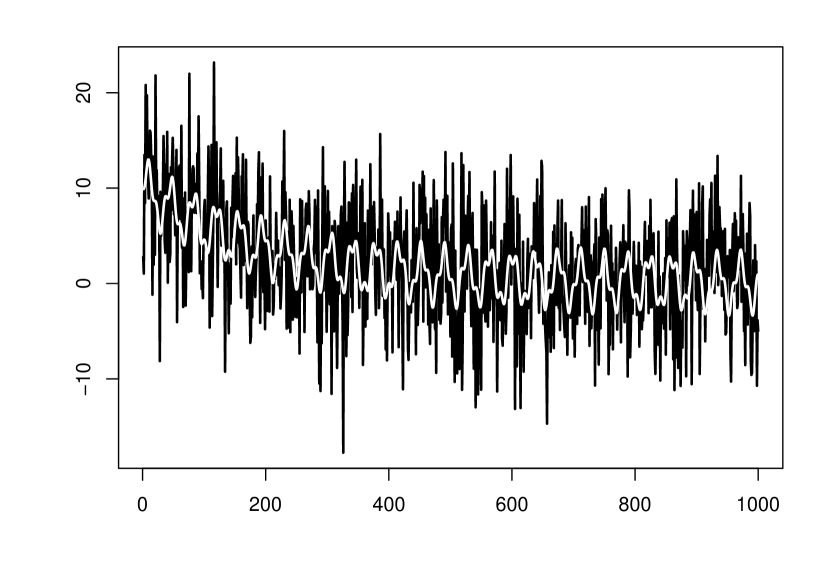
Figure 3: The Series $F_{1000}$ and $F^{\prime}_{1000}$.

We compare $3$ different SSA implementations: one uses the full SVD via DGESDD routine from ATLAS library, another one uses the full SVD via the same routine from ACML library and third uses fast Hankel truncated SVD and FFT-based rank-1 hankelization. Again, FFTW library was used to perform the FFT. Window size for SSA was always fixed at half of the series length.

Figure 4: Reconstruction Time Comparison.

The running times for the rank $5$ reconstruction are presented on the figure 4. Note that logarithmic scale was used for the y-axis. From it we can easily see that the running times for the SSA implementation via fast Hankel SVD and FFT-based rank-1 hankelization are dramatically smaller compared to the running times of other implementations for any non-trivial series length.

6.4 Detection of Structural Changes

The SSA can be used to detect the structural changes in the series. The main instrument here is so-called heterogeneity matrix (H-matrix). We will briefly describe the algorithm for construction of such matrix, discuss the computation complexity of the contruction and compare the performances of different implementations.

Exhaustive exposition of the detection of structural changes by the means of SSA can be found in [14].

Consider two time series $F^{(1)}$ and $F^{(2)}$. Let $N_{1}$ and $N_{2}$ denote their lengths respectively. Take integer $L<\min\left(N_{1}-1,N_{2}\right)$. Let $U_{j}^{(1)}$, $j=1,\dots,L$ denote the eigenvectors of the SVD of the trajectory matrix of the series $F^{(1)}$. Fix $I$ to be a subset of $\left\{1,\dots,L\right\}$ and denote $\mathcal{L}^{(1)}=\operatorname*{\mathrm{span}\,}\left(U_{i},\,i\in I\right)$. Denote by $X^{(2)}_{1},\dots,X^{(2)}_{K_{2}}$ ($K_{2}=N_{2}-L+1$) the $L$-lagged vectors of the series $F^{(2)}$.

Now we are ready to introduce the heterogeneity index [14] which measures the descrepancy between the series $F^{(2)}$ and the structure of the series $F^{(1)}$ (this structure is described by the subspace $\mathcal{L}^{(1)}$):

$$g(F^{(1)},F^{(2)})=\frac{\sum_{j=1}^{K_{2}}{\operatorname*{\mathrm{dist}\,}^{2}\left(X^{(2)}_{j},\mathcal{L}^{(1)}\right)}}{\sum_{j=1}^{K_{2}}{\left\|X^{(2)}_{j}\right\|^{2}}},$$ (10)

where $\operatorname*{\mathrm{dist}\,}(X,\mathcal{L})$ denotes the Euclidian distance between the vector $X$ and subspace $\mathcal{L}$. One can easily see that $0\leq g\leq 1$.

Note that since the vectors $U_{i}$ form the orthonormal basis of the subspace $\mathcal{L}^{(1)}$ equation (10) can be rewritten as

$$g(F^{(1)},F^{(2)})=1-\frac{\sum_{j=1}^{K_{2}}{\sum_{i\in I}}{\left(U_{i}^{T}X^{(2)}_{j}\right)^{2}}}{\sum_{j=1}^{K_{2}}{\left\|X^{(2)}_{j}\right\|^{2}}}.$$

Having this descrepancy measure for two arbitrary series in the hand one can obviously construct the method of detection of structural changes in the single time series. Indeed, it is sufficient to calculate the heterogeneity index $g$ for different pairs of subseries of the series $F$ and study the obtained results.

The heterogeneity matrix (H-matrix) [14] provides a consistent view over the structural descrepancy between different parts of the series. Denote by $F_{i,j}$ the subseries of $F$ of the form: $F_{i,j}=\left(f_{i},\dots,f_{j}\right)$. Fix two integers $B>L$ and $T\geq L$. These integers will denote the lengths of base and test subseries correspondingly. Introduce the H-matrix $G_{B,T}$ with the elements $g_{ij}$ as follows:

$$g_{ij}=g(F_{i,i+B},F_{j,j+T}),$$

for $i=1,\dots,N-B+1$ and $j=1,\dots,N-T+1$. In simple words we split the series $F$ into subseries of lengths $B$ and $T$ and calculate the heteregoneity index between all possible pairs of the subseries.

The computation complexity of the calculation of the H-matrix is formed by the complexity of the $SVDs$ for series $F_{i,i+B}$ and complexity of calculation of all heteregeneity indices $g_{ij}$ as defined by equation (10).

The worst-case complexity of the SVD for series $F_{i,i+B}$ corresponds to the case when $L\sim B/2$. Then the single decomposition costs $O(B^{3})$ for full SVD via Golub-Reinsh method and $O(kB\log{B}+k^{2}B)$ via fast Hankel SVD as presented in sections 3 and 4. Here $k$ denotes the number of elements in the index set $I$. Since we need to make $N-B+1$ decompositions a total we end with the following complexities of the worst case (when $B\sim N/2$): $O(N^{4})$ for full SVD and $O(kN^{2}\log{N}+k^{2}N^{2})$ for fast Hankel SVD.

Having all the desired eigenvectors $U_{i}$ for all the subseries $F_{i,i+B}$ in hand one can calculate the H-matrix $G_{B,T}$ in $O(kL(T-L+1)(N-T+1)+(N-T+1)L)$ multiplications. The worst case corresponds to $L\sim T/2$ and $T\sim N/2$ yielding the $O(kN^{3})$ complexity for this step. We should note that this complexity can be further reduced with the help of fast Hankel matrix-vector multiplication, but for the sake of simplicity we won’t present this result here.

Summing the complexities we end with $O(N^{4})$ multiplications for H-matrix computation via full SVD and $O(kN^{3}+k^{2}N^{2})$ via fast Hankel SVD.

For the implementation comparison we consider the series $F_{N}=(f_{1},\dots,f_{N})$ of the form

$$f_{n}=\begin{cases}\sin\left(\frac{2\pi}{10}n\right)+0.01\varepsilon_{n},\quad&n<Q,\\ \sin\left(\frac{2\pi}{10.5}n\right)+0.01\varepsilon_{n},\quad&n\geq Q,\end{cases}$$ (11)

where $\varepsilon_{n}$ denotes the uncorrelated white noise.

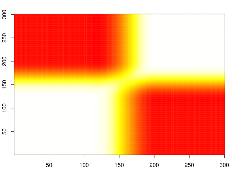
Figure 5: H-matrix for the series (11).

The typical H-matrix for such series is shown on the figure 5 (compare with figure 3.3 in [14]). The parameters used for this matrix are $N=400$, $Q=200$, $B=100$, $T=100$, $L=50$ and $I=\left\{1,2\right\}$.

To save some computational time we compared not the worst case complexities, but some intermediate situation. The parameters used were $Q=N/2$, $B=T=N/4$, $L=B/2$ and $I=\left\{1,2\right\}$. For full SVD DGESDD routine from ATLAS library [29] was used (as it was shown below, it turned out to be the fastest full SVD implementation available for our platform).

The obtained results are shown on the figure 6. As before, logarithmic scale was used for the y-axis. Notice that the implementation of series structure change detection using fast Hankel SVD is more than $10$ times faster even on series of moderate length.

Figure 6: Structure Change Detection Comparison

7 Real-World Time Series

Fast SSA implementation allows us to use large window sizes during the decomposition, which was not available before. This is a crucial point in the achieving of asymptotic separability between different components of the series [14].

7.1 Trend Extraction for HadCET dataset

Hadley Centre Central England Temperature (HadCET) dataset [22] is the longest instrumental record of temperature in the world. The mean daily data begins in $1772$ and is representative of a roughly triangular area of the United Kingdom enclosed by Lancashire, London and Bristol. Total series length is $86867$ (up to October, 2009).

We applied SSA with the window length of $43433$ to obtain the trend and few seasonal components. The decomposition took $22.5$ seconds and $50$ eigentriples were computed. First eigentriple was obtained as a representative for the trend of the series. The resulting trend on top of 5-year running mean temperature anomaly relative to $1951$-$1980$ is shown on figure 7 (compare with figure $1$ in [17]).

Figure 7: Hadley CET Series and Extracted Trend

7.2 Quebec Birth Rate Series

The series obtained from [18] contains the number of daily births in Quebec, Canada, from January 1, 1977 to December 31, 1990. They were discussed in [14] and it was shown that in addition to a smooth trend, two cycles of different ranges: the one-year periodicity and the one-week periodicity can be extracted from the series.

However, the extraction of the year periodicity was incomplete since the series turned out to be too smooth and do not uncover the complicated structure of the year periodicity (for example, it does not contain the birth rate drop during the Christmas). Total series length is $5113$, which suggests the window length of $2556$ to be used to achieve the optimal separability. This seems to have been computationaly expensive at the time of book written (even nowadays the full SVD of such matrix using LAPACK takes several minutes and requires decent amount of RAM).

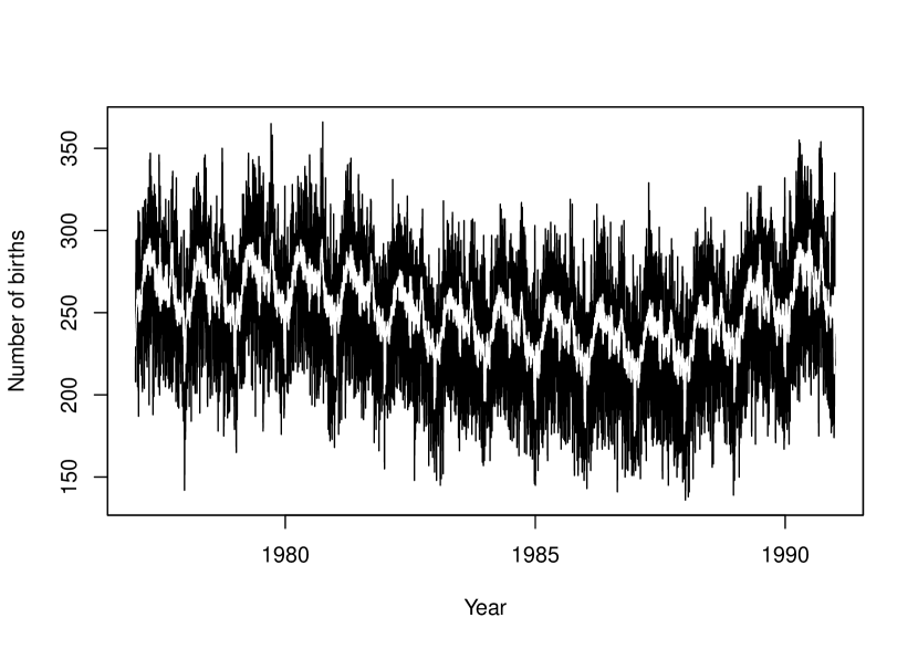
Figure 8: Quebec Birth Rate: Trend and Year Periodicity

We apply the sequential SSA approach: first we did the decomposition using window size of $365$. This allows us to extract the trend and week periodicity in the same way as described in [14]. After that we performed the decomposition of the residual series using the window length of $2556$. $100$ eigentriples were computed in $3.2$ seconds. The decomposition cleanly revealed the complicated structure of the year periodicity: we identified many components corresponding to the periods of year, half-year, one third of the year, etc. In the end, the eigentriples $1-58$ excluding $22-24$ were used during the reconstruction. The end result containing trend and year periodicity is shown on the figure 8 (compare with figure $1.9$ in [14]). It explains the complicated series structure much better.

8 Conclusion

The stages of the basic SSA algorithm were reviewed and their computational and space complexities were discussed. It was shown that the worst-case computational complexity of $O(N^{3})$ can be reduced to $O(kN\log{N}+k^{2}N)$, where $k$ is the number of desired eigentriples.

The implementation comparison was presented as well showing the superiority of the outlined algorithms in the terms of running time. This speed improvement enables the use of the SSA algorithm for the decomposition of quite long time series using the optimal for asymptotic separability window size.

References

- [1] Anderson, E., Bai, Z., Bischof, C., Blackford, S., Demmel, J., Dongarra, J., Du Croz, J., Greenbaum, A., Hammarling, S., McKenney, A., and Sorensen, D. (1999). LAPACK Users’ Guide, Third ed. Society for Industrial and Applied Mathematics, Philadelphia, PA.
- [2] Badeau, R., Richard, G., and David, B. (2008). Performance of ESPRIT for estimating mixtures of complex exponentials modulated by polynomials. Signal Processing, IEEE Transactions on 56, 2 (Feb.), 492–504.
- [3] Baglama, J. and Reichel, L. (2005). Augmented implicitly restarted Lanczos bidiagonalization methods. SIAM J. Sci. Comput. 27, 1, 19–42.
- [4] Briggs, W. L. and Henson, V. E. (1995). The DFT: An Owner’s Manual for the Discrete Fourier Transform. SIAM, Philadelphia.
- [5] Browne, K., Qiao, S., and Wei, Y. (2009). A Lanczos bidiagonalization algorithm for Hankel matrices. Linear Algebra and Its Applications 430, 1531–1543.
- [6] Chan, R. H., Nagy, J. G., and Plemmons, R. J. (1993). FFT-Based preconditioners for Toeplitz-block least squares problems. SIAM Journal on Numerical Analysis 30, 6, 1740–1768.
- [7] Dhillon, I. S. and Parlett, B. N. (2004). Multiple representations to compute orthogonal eigenvectors of symmetric tridiagonal matrices. Linear Algebra and its Applications 387, 1 – 28.
- [8] Djermoune, E.-H. and Tomczak, M. (2009). Perturbation analysis of subspace-based methods in estimating a damped complex exponential. Signal Processing, IEEE Transactions on 57, 11 (Nov.), 4558–4563.
- [9] Frigo, M. and Johnson, S. G. (2005). The design and implementation of FFTW3. Proceedings of the IEEE 93, 2, 216–231. Special issue on ‘‘Program Generation, Optimization, and Platform Adaptation’’.
- [10] Golub, G. and Kahan, W. (1965). Calculating the singular values and pseudo-inverse of a matrix. SIAM J. Numer. Anal 2, 205–224.
- [11] Golub, G. and Loan, C. V. (1996). Matrix Computations, 3 ed. Johns Hopkins University Press, Baltimore.
- [12] Golub, G. and Reinsch, C. (1970). Singular value decomposition and least squares solutions. Numer. Math. 14, 403–420.
- [13] Golyandina, N. (2009). Approaches to parameter choice for SSA-similar methods. Unpublished manuscript.
- [14] Golyandina, N., Nekrutkin, V., and Zhiglyavsky, A. (2001). Analysis of time series structure: SSA and related techniques. Monographs on statistics and applied probability, Vol. 90. CRC Press.
- [15] Golyandina, N. and Usevich, K. (2009). 2D-extensions of singular spectrum analysis: algorithm and elements of theory. In Matrix Methods: Theory, Algorithms, Applications. World Scientific Publishing, 450–474.
- [16] Gu, M. and Eisenstat, S. C. (1995). A divide-and-conquer algorithm for the bidiagonal SVD. SIAM J. Matrix Anal. Appl. 16, 1, 79–92.
- [17] Hansen, J., Sato, M., Ruedy, R., Lo, K., Lea, D. W., and Elizade, M. M. (2006). Global temperature change. Proceedings of the National Academy of Sciences 103, 39 (September), 14288–14293.
- [18] Hipel, K. W. and Mcleod, A. I. (1994). Time Series Modelling of Water Resources and Environmental Systems. Elsevier, Amsterdam. http://www.stats.uwo.ca/faculty/aim/1994Book/.
- [19] Larsen, R. M. (1998). Efficient algorithms for helioseismic inversion. Ph.D. thesis, University of Aarhus, Denmark.
- [20] Loan, C. V. (1992). Computational frameworks for the fast Fourier transform. Society for Industrial and Applied Mathematics, Philadelphia, PA, USA.
- [21] O’Leary, D. and Simmons, J. (1981). A bidiagonalization-regularization procedure for large scale discretizations of ill-posed problems. SIAM J. Sci. Stat. Comput. 2, 4, 474–489.
- [22] Parker, D. E., Legg, T. P., and Folland, C. K. (1992). A new daily central England temperature series. Int. J. Climatol 12, 317–342.
- [23] Parlett, B. (1980). The Symmetric Eigenvalue Problem. Prentice-Hall, New Jersey.
- [24] Parlett, B. and Reid, J. (1981). Tracking the progress of the Lanczos algorithm for large symmetric eigenproblems. IMA J. Numer. Anal. 1, 2, 135–155.
- [25] R Development Core Team. (2009). R: A Language and Environment for Statistical Computing. R Foundation for Statistical Computing, Vienna, Austria. ISBN 3-900051-07-0, http://www.R-project.org.
- [26] Simon, H. (1984a). Analysis of the symmetric Lanczos algorithm with reothogonalization methods. Linear Algebra Appl. 61, 101–131.
- [27] Simon, H. (1984b). The Lanczos algorithm with partial reorthogonalization. Math. Comp. 42, 165, 115–142.
- [28] Swarztrauber, P., Sweet, R., Briggs, W., Hensen, V. E., and Otto, J. (1991). Bluestein’s FFT for arbitrary N on the hypercube. Parallel Comput. 17, 607–617.
- [29] Whaley, R. C. and Petitet, A. (2005). Minimizing development and maintenance costs in supporting persistently optimized BLAS. Software: Practice and Experience 35, 2 (February), 101–121.
- [30] Wu, K. and Simon, H. (2000). Thick-restart Lanczos method for large symmetric eigenvalue problems. SIAM J. Matrix Anal. Appl. 22, 2, 602–616.
- [31] Yamazaki, I., Bai, Z., Simon, H., Wang, L.-W., and Wu, K. (2008). Adaptive projection subspace dimension for the thick-restart Lanczos method. Tech. rep., Lawrence Berkeley National Laboratory, University of California, One Cyclotron road, Berkeley, California 94720. October.