Time Delays in the Gravitationally Lensed Quasar H1413+117 (Cloverleaf)

Abstract

The quadruple quasar H1413+117 ($z_{s}$ = 2.56) has been monitored with the 2.0 m Liverpool Telescope in the $r$ Sloan band from 2008 February to July. This optical follow–up leads to accurate light curves of the four quasar images (A–D), which are defined by 33 epochs of observation and an average photometric error of $\sim$ 15 mmag. We then use the observed (intrinsic) variations of $\sim$ 50$-$100 mmag to measure the three time delays for the lens system for the first time (1$\sigma$ confidence intervals): $\Delta\tau_{AB}$ = $-$17 $\pm$ 3, $\Delta\tau_{AC}$ = $-$20 $\pm$ 4, and $\Delta\tau_{AD}$ = 23 $\pm$ 4 days ($\Delta\tau_{ij}=\tau_{j}-\tau_{i}$; B and C are leading, while D is trailing). Although time delays for lens systems are often used to obtain the Hubble constant ($H_{0}$), the unavailability of the spectroscopic lens redshift ($z_{l}$) in the system H1413+117 prevents a determination of $H_{0}$ from the measured delays. In this paper, the new time delay constraints and a concordance expansion rate ($H_{0}$ = 70 km s^-1 Mpc^-1) allow us to improve the lens model and to estimate the previously unknown $z_{l}$. Our 1$\sigma$ estimate $z_{l}$ = 1.88${}^{+0.09}_{-0.11}$ is an example of how to infer the redshift of very distant galaxies via gravitational lensing.

1. Introduction

The time delay between two images of a gravitationally lensed source depends on the distribution of mass in the lens and the current expansion rate of the Universe (Refsdal, 1964, 1966). This expansion rate is quantified by the Hubble constant $H_{0}$. If the source is a quasar, the intrinsic quasar variability may be used to determine the time delays between its multiple images. Thus, observed delays for lensed quasars lead to valuable information on $H_{0}$, provided lensing mass distributions can be constrained by observational data (e.g., Kochanek & Schechter, 2004; Schechter, 2004; Saha et al., 2006; Jackson, 2007; Oguri, 2007). Future large samples of lens systems could be useful tools to obtain accurate estimates of the main cosmological parameters (e.g., Dobke et al., 2009).

For a given lensed quasar, each time delay between two of its images is indeed scaled by a factor containing $H_{0}$, the lens redshift $z_{l}$, and additional physical parameters. If $z_{l}$ is known (this is the usual situation), the Hubble constant and the lensing mass distribution can be simultaneously deduced by using a parametric lens scenario and a set of observational constraints (including information on the time delay(s); e.g., Schneider et al., 2006). However, a large set of constraints is required to reliably determine both cosmological and galactic properties.

Accurate observations of a quadruply imaged quasar in a well–studied galaxy field bring an excellent opportunity to study in detail $H_{0}$ and the mass distribution of the gravitational lens. Apart from the three independent time delays, and the positions and fluxes of the four images, data on the neighbour galaxies also constraint the lens scenario (e.g., Jackson, 2007). Alternatively, if $z_{l}$ is very uncertain or unknown, one may infer a lens redshift value from the time delay measurements and the rest of constraints (using a value of $H_{0}$ from other experiments).

In this paper we focus on the quadruple quasar H1413+117 (catalog ) (Cloverleaf; Magain et al., 1988), lying at a redshift $z_{s}$ = 2.558 (e.g., Barbainis et al., 1997). Although the lens redshift is currently unknown, several neighbour galaxies were detected by Kneib et al. (1998). Kneib et al. (1998) found the main lensing galaxy G1 amid the four quasar images, and presented astrometric and photometric data for additional galaxies surrounding H1413+117 (catalog ). They analysed a secondary lensing galaxy (G2) close to G1, as well as some other objects probably belonging to an overdensity (galaxy group/cluster) at photometric redshift $z_{ove}\sim$ 0.9. Faure et al. (2004) also found evidence for the presence of two different overdensities at $z_{ove}$ = 0.8 $\pm$ 0.3 (corresponding to the structure discovered by Kneib et al., 1998) and $z_{ove}$ = 1.75 $\pm$ 0.2, which could contribute noticeably to the lensing potential.

Very recently, MacLeod et al. (2009) have used the positions of G1, G2, and other candidate lensing galaxies, the quasar image positions (Turnshek et al., 1997), new mid–IR flux ratios, and some priors to constrain the lensing mass distribution. They have concluded that the galaxy pair G1–G2 and an external shear (likely related to the observed galaxy overdensities) are required to explain the observations. From an optical monitoring over the 1987–94 period, Ostensen et al. (1997) also reported a quasi–simultaneous variability of the four quasar images. Unfortunately, the scarce sampling did not permit them to estimate the time delays in the system. Hence, the measurement of time delays for the Cloverleaf quasar should improve knowledge about the lens (mass and redshift), as well as allow completion of new studies (e.g., microlensing variability).

In Section 2 we present new optical light curves of H1413+117 (catalog ). In Section 3, from these light curves, we estimate the time delays between quasar images. In Section 4 we compare the most recent lens scenario with all relevant observations. In Section 5 we discuss our results and put them into perspective.

2. Observations and light curves

We observed H1413+117 (catalog ) from early February to late July of 2008, i.e., for 6 months. All observations were made with the 2.0 m fully robotic Liverpool Telescope (LT) at the Roque de los Muchachos Observatory, Canary Islands (Spain), using the RATCam optical CCD camera (binning 2 $\times$ 2). The global database consists of 61 exposures of 300 s in the $r$ Sloan filter. These original exposures (frames) are almost regularly distributed over the whole observation period (there is only a significant 21–day gap in 2008 February), with an average sampling rate of about one frame each three days. In Fig. 1, a combined LT frame shows the blended quasar images (at the centre of the field), two relevant stars (the control star S40 and the PSF star S45, which correspond to the objects 40 and 45 in Fig. 1 of Kayser et al., 1990), and other relatively bright objects. The left bottom corner of Fig. 1 illustrates the positions (crosses) and names (A–D) of the four quasar images.

The four quasar images are separated by $\sim 1\arcsec$ (see Fig. 1), so we only consider 33 high–quality frames to make the light curves (photometry on the other 28 frames is discussed in the last paragraph of Section 3). This selection is based on the FWHM of the seeing disc measured in each frame (FWHM $<1\farcs 5$), as well as the signal–to–noise ratio (SNR) of the 18.16–mag control star (SNR $>$ 150). We note that this star (S40 in Fig. 1) has an $r$–band brightness similar to those of the quasar images ($\sim$ 17.9–18.4 mag). Each SNR value is calculated within an aperture with radius equal to the frame FWHM.

We determine the instrumental fluxes of the four quasar images through point–spread function (PSF) fitting. As the main lensing galaxy is very faint in the $r$ band ($R>$ 22.7 mag; Kneib et al., 1998), our photometric model includes four stellar–like sources (i.e., 4 empirical PSFs) plus a constant background. The empirical PSF is derived from the 16.69–mag star in the vicinity of the lens system (S45 in Fig. 1). In order to obtain accurate and reliable fluxes, we use the well–tested IMFITFITS software (McLeod et al., 1998), incorporating the relative positions of the B–D images (with respect to A; Turnshek et al., 1997) as constraints. Thus, the code is applied to all selected frames (see above), allowing 7 parameters to be free. These free parameters are the position of the A image, the fluxes of the A–D images, and the sky brightness. We also infer SDSS magnitudes from the relative instrumental magnitudes of the lensed quasar. The S45 star is taken as reference for differential photometry. In Table 1 we present the $r$–SDSS magnitudes of the four images and the control (S40) star.

From the standard deviation of the magnitudes of the S40 star over the whole monitoring period, we obtain a typical error of 0.006 mag. This global scatter agrees with the standard deviation between magnitudes on consecutive nights divided by the square root of 2, as expected on theoretical grounds. To estimate typical photometric errors in the quasar light curves, we then use the standard deviations between magnitudes having time separations $<$ 1.5 days (true variability is negligible on this very short timescale), which are divided by the square root of 2. The resulting uncertainties are 0.010 (A), 0.012 (B), 0.018 (C) and 0.018 (D) mag. As a summary, we achieve $\sim$ 1–2% photometry and reasonable sampling rate ($\sim$ 6 data per month). Moreover, the light curves of the A–D images show significant variations of $\sim$ 0.05–0.1 mag (see Fig. 2). For example, the almost parallel fading by $\sim$ 0.1 mag of A–D (over the last 100 days in Fig. 2) suggests intrinsic variability. This is promising to derive time delays.

3. Time delays

There are four different image ray paths for the Cloverleaf quasar, so traveltime ($\tau$) varies from image to image (Schneider et al., 1992). Assuming that the observed magnitude fluctuations are basically originated in the source quasar (intrinsic variability), we use two well–known cross–correlation techniques to measure time delays between quasar images $\Delta\tau_{ij}=\tau_{j}-\tau_{i}$, where $i,j=A,B,C,D$. These techniques are the dispersion ($D^{2}$) and reduced chi–square ($\hat{\chi}^{2}$) minimizations (e.g., Pelt et al., 1996; Ullán et al., 2006). Despite the existence of other methods for determining time delays (e.g., Kundić et al., 1997; Gil-Merino et al., 2002), most methods work in a similar way, and in most cases one does not need to carry out an exhaustive analysis. After deriving delays we discuss the intrinsic variability hypothesis at the end of this section.

We focus on the AB, AC, and AD comparisons, i.e., the A light curve is compared to the other three brightness records (B–D). The $D^{2}$ and $\hat{\chi}^{2}$ minimizations are characterized by a decorrelation length ($\delta$) and a bin semisize ($\alpha$), respectively. To simultaneously avoid very noisy trends and loss of signal (due to excessive smoothing), we take $\alpha$ = $\delta$ = 15 days. For $\alpha$ = $\delta$ = 15 days, the spectra between $-$75 and +75 days include global and local minima. However, these local minima do not play an important role in the estimation of the time delays $\Delta\tau_{AB}$, $\Delta\tau_{AC}$, and $\Delta\tau_{AD}$ (see below).

For a given cross–correlation method, we follow two different approaches to generate synthetic light curves and determine time delay errors. In the first approach (which is called NORMAL), we do not make any hypothesis on the underlying signal, but the observational noises (in the four light curves) are assumed to be normally distributed. Therefore, one obtains a synthetic light curve of an image by adding a random quantity to each brightness in the observed record. These random quantities are realizations of a normal distribution around zero, with a standard deviation equal to the standard deviation between observed magnitudes on consecutive nights. We produce 1000 synthetic light curves of each image, and thus, obtain 1000 delay values for each pair (AB, AC, and AD) and the corresponding 68% confidence intervals. In the second approach, we use a bootstrap procedure (BOOTSTRAP; e.g., Efron & Tibshirani, 1993). First, we derive a combined light curve from the best solutions of $\Delta\tau_{AB}$, $\Delta\tau_{AC}$, and $\Delta\tau_{AD}$ (global minima of the three spectra), and the associated magnitude differences. This combined curve is then smoothed by a 20–day filter. Second, the combined and smoothed curve is assumed to be a rough reconstruction of the underlying signal, and thus, the residuals for each image are taken as sets of errors. These four sets are resampled to infer 1000 bootstrap simulations (synthetic light curves) of each image. To measure the time delays (68% confidence intervals), we compute 1000 delay values for each pair of images and analyse the three distributions.

The time delay measurements are presented in Table 2. For each pair of images, the four measurements are consistent with each other. Table 2 also indicates the existence of an average offset of about 3 days between the results from the NORMAL approach and those derived from BOOTSTRAP simulations. This offset may be due to slightly biased reconstructions of the underlying signal (BOOTSTRAP procedure). We adopt $\Delta\tau_{AB}$ = $-$17 $\pm$ 3, $\Delta\tau_{AC}$ = $-$20 $\pm$ 4, and $\Delta\tau_{AD}$ = 23 $\pm$ 4 days as our final 1$\sigma$ measurements ($\hat{\chi}^{2}$ and NORMAL). The corresponding $r$–band magnitude differences are $\Delta m_{AB}$ = 0.155 $\pm$ 0.006, $\Delta m_{AC}$ = 0.322 $\pm$ 0.011, and $\Delta m_{AD}$ = 0.501 $\pm$ 0.007 mag (1$\sigma$ confidence intervals). These give the magnification (flux) ratios: $B/A$ = 0.867 $\pm$ 0.005, $C/A$ = 0.743 $\pm$ 0.007, and $D/A$ = 0.630 $\pm$ 0.004.

From the central values in the time delay and magnitude difference intervals, one can obtain a final combined light curve, i.e., the A light curve together with the magnitude– and time–shifted B–D records. In Fig. 3 we display this combined light curve (filled symbols). Using a 20–day filter (filter semisize = 10 days), a possible reconstruction of the underlying intrinsic signal is also drawn in Fig. 3 (solid line). The standard deviation between the magnitudes in the combined record and the reconstruction is about 0.015 mag (see the shaded area in Fig. 3, which represents 0.015–mag deviations from the reconstruction), in good agreement with the average photometric error in the quasar light curves (see the error bar in the lower left corner of Fig. 3). This suggests the absence of significant microlensing signals, and strengthens our hypothesis that observed variations mainly have an intrinsic origin. We also note that Ostensen et al. (1997) reported on an almost parallel variation in brightness ($R$ band) of the four quasar images over a 7–year period (see the middle panels in Figs. 2–3 of that paper). Moreover, our 6–month monitoring period was long enough to find significant variability and determine time delays, but it was not long enough to detect substantial microlensing variations. Typical microlensing gradients of $\sim$ 10^-4 mag day^-1 are expected in the $rR$ bands (e.g., Gaynullina et al., 2005; Fohlmeister et al., 2007; Shalyapin et al., 2009).

Once the time delays are measured and the combined light curve is drawn in Fig. 3 (filled symbols), we can discuss the accuracy of the magnitudes derived from the poor–quality frames (see Section 2). These 28 exposures with FWHM $\geq 1\farcs 5$ and/or SNR $\leq$ 150 seem to be useless, since they lead to a very noisy combined record and confusion. One frame has a very poor image quality, so we do not extract quasar magnitudes. Some of the magnitudes associated with the other 27 poor–quality frames are shown in Fig. 3 (open symbols). The rest are extremely noisy, and their values are outside the magnitude range in Fig. 3. In brief, 28 out of the 61 original frames have either an excessive blurring, or an insufficient signal, or both of them, so they do not produce accurate quasar light curves.

4. Improved lens model and lens redshift

In a model–independent way, the image and main lens positions for the H1413+117 (catalog ) system are useful to determine the ordering of the time delays (Saha & Williams, 2003). However, the quasar images B and C (associated with minimum arrival times) are almost equidistant from the main lens, so it is difficult to distinguish the leading image in this system. In any case, intrinsic variations should be firstly observed in light curves of these two images, and later in records of A and D. While D is the trailing image (it is the closest to the main lens), A should be characterized by an intermediate arrival time. Our time delay measurements agree with this time–ordering of the images. Detailed lens models predict that C is leading (Chae & Turnshek, 1999; MacLeod et al., 2009). However, we cannot confirm this prediction at 1$\sigma$ confidence level, since the $\Delta\tau_{AB}$ and $\Delta\tau_{AC}$ intervals overlap each other (a direct measure $\Delta\tau_{BC}$ is neither useful to decide on the leading image).

MacLeod et al. (2009) reported how a relatively simple lens model reproduces the observed positions and mid–IR flux ratios of the four quasar images. These mid–IR flux ratios are insensitive to extinction (long wavelength) and microlensing (large emission region). The MacLeod et al.’s main solution (see the second column in Table 3) relies on an observationally motivated scenario. This consists of a background point–like source (quasar) that is lensed by a singular isothermal ellipsoid (main lensing galaxy G1), a singular isothermal sphere (secondary lensing galaxy G2), and an external shear (likely produced by galaxy overdensities; Kneib et al., 1998; Faure et al., 2004). Although the position of G1 was constrained by observations, it was allowed to vary during the fitting procedure. The singular isothermal sphere was placed at the observed position of G2, and MacLeod et al. also assumed priors on the ellipticity of G1 ($e_{G1}$ = 0.0 $\pm$ 0.5) and the strength of the external shear ($\gamma_{ext}$ = 0.05 $\pm$ 0.05).

Here, we use the MacLeod et al.’s lens scenario and a concordance cosmology: $H_{0}$ = 70 km s^-1 Mpc^-1, $\Omega_{m}$ = 0.3, $\Omega_{\Lambda}$ = 0.7 (e.g., Spergel et al., 2003). The theoretical time delay between two lensed images includes a cosmological scale factor $T=(1+z_{l})(D_{l}D_{s}/cD_{ls})$, where $c$ is the velocity of light and $D$ denotes angular diameter distance (e.g., Schneider et al., 1992). The angular diameter distances are determined by the cosmology, and the lens and source redshifts, $z_{l}$ and $z_{s}$. Thus, using a concordance cosmology and the observed redshift of the source $z_{s}$ = 2.558 (e.g., Barbainis et al., 1997), the scale factor exclusively depends on $z_{l}$. Our goal is to find a good fit to all observations of interest, i.e., the image positions and (mid–IR) fluxes, and the three time delays in Section 3. We also use the constraints and priors on the G1–G2 positions, $e_{G1}$, and $\gamma_{ext}$ by MacLeod et al. (2009). With respect to the MacLeod et al.’s framework, we add 3 new observational constraints (time delays) and one new free parameter ($z_{l}$), so the degrees of freedom (dof) change from 5 to 7.

Through the GRAVLENS software package (Keeton, 2001), we find a solution with $\chi^{2}$/dof = 7.5/7. Our main results are shown in the third column of Table 3. Most lensing mass parameters of this acceptable solution are close (deviations less than 10%) to those in the second column of the same table (see also the third column in Table 3 of MacLeod et al., 2009). However, it is interesting to note that the new external shear strength ($\gamma_{ext}$ = 0.11) is slightly larger than the previous one, whereas the mass scale of G2 ($b_{G2}=0\farcs 45$) is slightly smaller (deviations of 25–30%). On the other hand, the best–fit lens redshift indicates the existence of a very distant galaxy pair G1–G2. In Fig. 4 we draw the $\chi^{2}-z_{l}$ relationship, which permits us to obtain confidence intervals for $z_{l}$. The 1$\sigma$ determination is $z_{l}$ = 1.88${}^{+0.09}_{-0.11}$ (dark shaded area in Fig. 4). Fig. 4 also shows the 2$\sigma$ (95%) confidence interval: 1.65 $\leq z_{l}\leq$ 2.03 (whole shaded area).

5. Discussion

In the lens system H1413+117 (catalog ), the main lensing galaxy G1 is a very faint object ($R>$ 22.7 mag; Kneib et al., 1998), surrounded by four close and relatively bright quasar images ($R\sim$ 18 mag). Thus, it is very difficult to separate the spectrum of the galaxy from those of the quasar images. Moreover, the quasar spectra indicate the presence of intervening objects (absorption lines) at different redshifts less than $z_{s}$ = 2.56 (e.g., Monier et al., 1998, and references therein), so one cannot decide on the redshift of G1. The secondary lensing galaxy G2 and other galaxies in the vicinity of the lensed quasar are also very faint objects ($R>$ 23 mag; Kneib et al., 1998), and spectroscopic redshifts of these galaxies are not available yet. Photometric data of field galaxies are consistent with the presence of two galaxy overdensities at $z_{ove}$ = 0.8 $\pm$ 0.3 and $z_{ove}$ = 1.75 $\pm$ 0.2 (Kneib et al., 1998; Faure et al., 2004). For example, the galaxy G2 has a photometric redshift of about 2 (Kneib et al., 1998). Our gravitational lensing estimate of the redshift of G1–G2: $z_{l}$ = 1.88${}^{+0.09}_{-0.11}$ (1$\sigma$ interval), is in reasonable agreement with the photometric redshift of G2 and the most distant overdensity, as well as the absorption system at $z_{abs}$ = 1.87. However, the nearest group/cluster is far away from the principal gravitational deflector (galaxy pair G1–G2).

So far it is not considered a possible uniform external convergence, i.e., $\kappa_{ext}$ = 0. If $\kappa_{ext}\neq$ 0, then fits to $\kappa_{ext}$ = 0 lens scenarios (lens models with $\kappa_{ext}$ = 0) must be conveniently rescaled. Original estimates of $H_{0}$ (if that were the case) or $z_{l}$ (in our case) also require suitable corrections. This is because of the so–called mass sheet degeneracy (e.g., Falco et al., 1985; Gorenstein et al., 1988; Saha, 2000; Nakajima et al., 2009). For H1413+117 (catalog ), it is unclear what is the main perturber producing external shear, and perhaps external convergence. For example, infrared photometry of the neighbour galaxy H2 is consistent with a redshift of about 2 (Kneib et al., 1998), so it could be located in the principal lens plane. Moreover, the orientation of the external shear, $\theta_{\gamma_{ext}}=45\fdg 4$, is in the direction of this galaxy (e.g., see Fig. 4 of MacLeod et al., 2009). Thus, H2 and some other related objects (belonging to the very distant overdensity) might produce most of the external shear and a negligible convergence. Apart from this optimistic perspective, one may also consider that the main perturber is the most distant group/cluster as a whole. If this were true, the external convergence at the quasar positions would be $\kappa_{ext}$ = $\gamma_{ext}\sim$ 0.1 for a singular isothermal sphere. Taking $\kappa_{ext}\sim$ 0.1 into account, the derived lens redshift increases by $\sim$ 3% (+ 0.05). This increase represents only one half of our 1$\sigma$ uncertainty in $z_{l}$ ($\sim$ 0.10; see above).

We can also quantify the gravitational influence of the nearest overdensity. A weak lensing analysis of this structure indicated a shear direction of $45\arcdeg$ (see the last column in Table 5 of Faure et al., 2004). This shear direction coincides with our strong lensing determination in Table 3, which suggests that the nearest overdensity might play a noticeble role in the lens phenomenon. Faure et al. (2004) also determined an upper limit on the shear strength: $\gamma<$ 0.17 (see Fig. 7 of Faure et al., 2004). Keeton (2003) and Momcheva et al. (2006) discussed the effective convergence and shear when a perturber does not lie at $z_{l}$, e.g., $z_{per}<z_{l}$. Assuming a singular isothermal sphere to describe the perturber, $\kappa_{eff}=\gamma_{eff}\sim(1-\beta)\gamma$, where $\beta\sim$ 0 if $z_{per}\sim z_{l}$ and $\beta>$ 0 if $z_{per}<z_{l}$ (see Appendix of Momcheva et al., 2006). From the involved redshifts and the upper limit on the shear strength, we infer that $\kappa_{eff}=\gamma_{eff}<$ 0.03. Thus, the nearest structure cannot account for the external shear in the lens system, and it likely generates no more than 10% of the total shear strength. The constraint on the effective convergence leads to a negligible increase in $z_{l}$, i.e., $\Delta z_{l}$ is below + 0.01. In some other lens systems, there are also perturbers at redshifts less than those of the principal lensing objects, which produce a few hundredths of external convergence and shear (e.g., Fassnacht & Lubin, 2002; Fassnacht et al., 2006).

Our lens scenario incorporates singular isothermal mass profiles. Despite the fact that these profiles lead to an acceptable fit ($\chi^{2}$/dof = 7.5/7), other distributions of mass (including a core, some deviation from the isothermal behaviour or both ingredients) could also lead to good fits for the observational data. This is the well–known profile degeneracy (e.g., Jackson, 2007). An exhaustive study of mass distributions consistent with the available observational constraints is out of the scope of this paper. However, we check the influence of non–isothermal profiles of G1 on $z_{l}$ estimations. The power–law index of G1 ($\alpha$) is assumed to be around 1 (isothermal index), and additional fits with singular $\alpha\neq 1$ profiles are done. For $\alpha$ = 1.1, the solution is characterized by $\Delta\chi^{2}=\chi^{2}-\chi^{2}(\alpha=1)$ = 0.1. For $\alpha$ = 0.8–0.9, we find a very modest improvement in $\chi^{2}$, $\Delta\chi^{2}$ = $-$0.1. The full range $\alpha$ = 0.8–1.1 leads to best–fit values of $z_{l}$ within our 1$\sigma$ ”isothermal” estimate in Section 4.

Microlensing variations in H1413+117 (catalog ) may shed light on the nature and structure of the source quasar (e.g., Lewis & Belle, 1998; Popović et al., 2006). The three time delay measurements in Section 3 and the new data on the lens (mass and redshift) in Section 4 are useful tools for analyses of microlensing variability. Once the delays are known, it is possible to properly compare quasar light curves and to search for microlensing signals. Moreover, the (lens and source) redshifts and the improved lens model allow construction of microlensing magnification patterns and simulated microlensing light curves (e.g., Wambsganss, 1990). The key parameters for microlensing simulations are the convergence and shear strength at the positions of the quasar images. To address the space distribution of both convergence and shear, we consider our lens model in the third column of Table 3. This gives ($\kappa_{A}$, $\gamma_{A}$) = (0.51, 0.58), ($\kappa_{B}$, $\gamma_{B}$) = (0.52, 0.32), ($\kappa_{C}$, $\gamma_{C}$) = (0.48, 0.37), and ($\kappa_{D}$, $\gamma_{D}$) = (0.57, 0.65). Although we cannot rule out the existence of an external convergence at a level of 0.1, this scenario is uncertain (see above). Hence, we do not take into account any external convergence due to galaxy overdensities along the line of sight to the lensed quasar.

Our lens model causes different magnifications at the four positions of the quasar images. The model magnification ratios are $B/A$ = 0.82, $C/A$ = 0.78, and $D/A$ = 0.45. All these ratios agree, as expected, with the mid–IR measurements by MacLeod et al. (2009). However, the model ratios are not included in the error bars of our optical ($r$–band) flux ratios in Section 3. These differences between optical and model ratios are probably due to dust extinction and microlensing magnification. If microlensing is currently playing a role (e.g., the optical continuum of the image D could be magnified by microlensing; Anguita et al., 2008, and references therein), it should be a long–term effect that induces small (optical) flux variations on time scales of several months. This microlensing variability scenario is supported by recent studies for other systems with non–local lens galaxies (e.g., Gaynullina et al., 2005; Fohlmeister et al., 2007; Shalyapin et al., 2009).

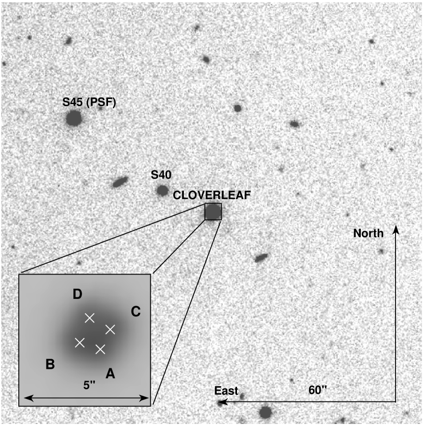
Figure 1.— $r$–band Liverpool Telescope imaging of the Cloverleaf quasar. We combine the 5 best frames in terms of seeing (total exposure time = 1500 s, FWHM = $0\farcs 87$). We then zoom into the central region and perform linear interpolation between adjacent pixels (box in the left bottom corner). The four quasar images and two relevant stars are properly labeled.

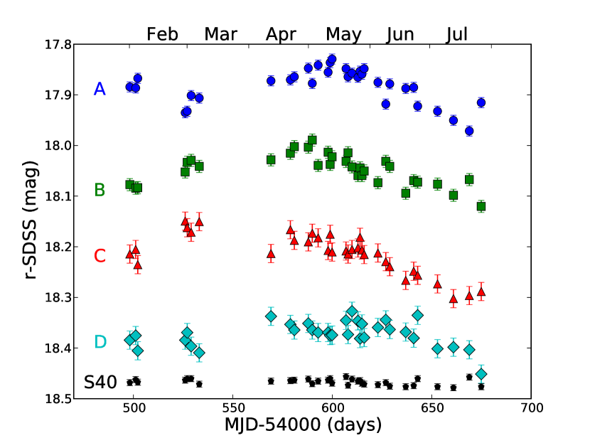
Figure 2.— Light curves of four quasar images A–D and the control star S40. The stellar record is shifted by +0.3 mag to facilitate comparison.

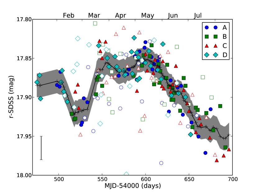
Figure 3.— Final combined light curve of H1413+117. This is made from the A light curve and the magnitude– and time–shifted B–D records (filled symbols). To create the combined record, we use the time delays $\Delta\tau_{AB}$ = $-$17, $\Delta\tau_{AC}$ = $-$20, and $\Delta\tau_{AD}$ = 23 days (shifts in time), and the magnitude differences $\Delta m_{AB}$ = 0.155, $\Delta m_{AC}$ = 0.322, and $\Delta m_{AD}$ = 0.501 mag (shifts in magnitude). We also display a possible reconstruction of the quasar signal (solid line), as well as the standard deviation between the combined record and the reconstruction (shaded area). The error bar in the lower left corner represents the average photometric error in the quasar light curves. To check the accuracy of the quasar magnitudes in 27 poor–quality frames that are not used in the time delay analysis, we also compare some of these additional magnitudes (open symbols) with those derived from the high–quality exposures (filled symbols). Several additional data (for the poor–quality frames) are outside the magnitude range from 18.0 to 17.8.

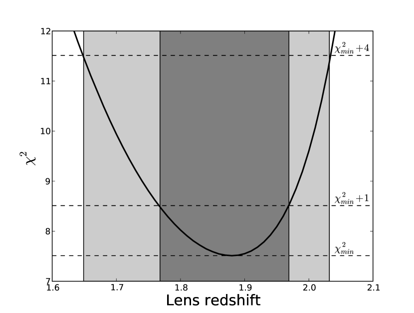
Figure 4.— Estimation of the previously unknown lens redshift. We show both the 1$\sigma$ (dark shaded area) and 2$\sigma$ (whole shaded area) confidence intervals. We estimate $z_{l}$ via gravitational lensing, using observational constraints on the lensed quasar images (positions, fluxes, and time delays), as well as data on the neighbour galaxies.

Table 1Photometry of H1413+117.

number	civil date	MJD-54000	FWHM	SNR	A	B	C	D	S40
1	Feb 1	498.1885	1.08	235	17.884	18.077	18.214	18.384	18.168
2	Feb 4	501.1370	1.07	232	17.886	18.084	18.205	18.375	18.162
3	Feb 5	502.1893	1.26	233	17.867	18.083	18.235	18.405	18.167
4	Feb 29	526.0175	1.45	164	17.935	18.052	18.149	18.384	18.163
5	Mar 1	527.0400	1.24	186	17.932	18.033	18.162	18.369	18.160
6	Mar 3	529.0227	1.44	173	17.901	18.029	18.171	18.396	18.160
7	Mar 7	533.0942	1.19	189	17.906	18.041	18.150	18.409	18.171
8	Apr 12	569.1711	1.31	192	17.872	18.028	18.213	18.337	18.165
9	Apr 22	578.9261	1.02	192	17.870	18.015	18.166	18.353	18.164
10	Apr 24	580.9120	1.32	202	17.864	18.002	18.187	18.364	18.163
11	May 1	587.9478	1.03	212	17.847	18.003	18.190	18.351	18.161
12	May 3	589.9377	1.22	210	17.877	17.989	18.173	18.364	18.170
13	May 6	592.8934	1.19	212	17.841	18.039	18.182	18.369	18.165
14	May 11	597.8990	1.27	192	17.855	18.013	18.207	18.369	18.163
15	May 12	598.9280	0.84	214	17.836	18.037	18.175	18.375	18.160
16	May 13	599.9053	1.04	167	17.829	18.022	18.210	18.374	18.169
17	May 20	606.9064	0.90	163	17.848	18.031	18.208	18.345	18.156
18	May 21	607.9159	1.09	182	17.864	18.014	18.214	18.373	18.173
19	May 23	609.9184	1.33	205	17.857	18.042	18.205	18.327	18.161
20	May 26	612.9050	1.15	220	17.865	18.059	18.202	18.346	18.165
21	May 27	613.9510	1.15	231	17.853	18.044	18.181	18.381	18.164
22	May 28	614.9155	0.87	238	17.859	18.059	18.206	18.352	18.169
23	May 29	616.0342	1.35	161	17.848	18.050	18.215	18.379	18.171
24	Jun 5	622.9486	1.19	238	17.875	18.073	18.212	18.359	18.172
25	Jun 9	626.9143	1.36	206	17.918	18.031	18.229	18.344	18.168
26	Jun 11	628.9096	0.84	196	17.878	18.041	18.239	18.363	18.175
27	Jun 19	636.9364	0.90	188	17.887	18.094	18.266	18.368	18.176
28	Jun 23	640.9468	1.24	228	17.885	18.069	18.248	18.380	18.174
29	Jun 25	642.9421	1.29	207	17.922	18.072	18.256	18.335	18.160
30	Jul 5	652.9233	1.17	232	17.932	18.076	18.273	18.401	18.176
31	Jul 13	660.9244	1.06	157	17.950	18.098	18.302	18.398	18.178
32	Jul 21	668.9129	1.29	164	17.971	18.067	18.296	18.403	18.157
33	Jul 27	674.9026	1.27	202	17.915	18.120	18.288	18.451	18.176

Table 2Time delays (in days) of H1413+117.

Method	Simulations	$\Delta\tau_{AB}$	$\Delta\tau_{AC}$	$\Delta\tau_{AD}$
$D^{2}$	NORMAL	$-$17${}^{+3}_{-5}$	$-$19 $\pm$ 6	24${}^{+5}_{-6}$
	BOOTSTRAP	$-$18 $\pm$ 3	$-$23${}^{+5}_{-7}$	20 $\pm$ 5
$\hat{\chi}^{2}$	NORMAL	$-$17 $\pm$ 3	$-$20 $\pm$ 4	23 $\pm$ 4
	BOOTSTRAP	$-$22${}^{+3}_{-4}$	$-$23${}^{+4}_{-7}$	21${}^{+4}_{-3}$

Note. — $\Delta\tau_{ij}=\tau_{j}-\tau_{i}$, so B and C are leading, and D is trailing. All measurements are 68% confidence intervals.

Table 3Modelling results.

Parameter	MacLeod et al. (2009)	This paper
$\chi^{2}$/dof	4.9/5	7.5/7
$b_{G1}$	$0\farcs 66$	$0\farcs 68$
$\Delta\alpha_{G1}$	$-0\farcs 166$	$-0\farcs 165$
$\Delta\delta_{G1}$	$0\farcs 556$	$0\farcs 552$
$e_{G1}$	0.26	0.28
$\theta_{e_{G1}}$	$-36\fdg 5$	$-37\fdg 6$
$b_{G2}$	$0\farcs 63$	$0\farcs 45$
$\Delta\alpha_{G2}$	$\equiv-1\farcs 87$	$\equiv-1\farcs 87$
$\Delta\delta_{G2}$	$\equiv 4\farcs 14$	$\equiv 4\farcs 14$
$\gamma_{ext}$	0.087	0.11
$\theta_{\gamma_{ext}}$	$50\fdg 1$	$45\fdg 4$
$z_{l}$	–	1.88

Note. — Position angles (ellipticity of G1 and external shear) are measured east of north and positions are relative to image A (negative $\Delta\alpha$ values are eastward of image A). Here, $b$, $e$, $\gamma$, and $z_{l}$ denote mass scale, ellipticity, shear strength, and lens redshift, respectively.

References

- Anguita et al. (2008) Anguita, T., Faure, C., Yonehara, A., Wambsganss, J., Kneib, J.-P., Covone, G., & Alloin, D. 2008, A&A, 481, 615
- Barbainis et al. (1997) Barbainis, R., Maloney, P., Antonucci, R., & Alloin, D. 1997, ApJ, 484, 695
- Chae & Turnshek (1999) Chae, K.-H., & Turnshek, D. A. 1999, ApJ, 51, 587
- Dobke et al. (2009) Dobke, B. M., King, L. J., Fassnacht,C. D., & Auger, M. W. 2009, MNRAS, 397, 311
- Efron & Tibshirani (1993) Efron, B., & Tibshirani, R. J. 1993, An Introduction to the Bootstrap (New York: Chapman & Hall)
- Falco et al. (1985) Falco, E. E., Gorenstein, M. V., & Shapiro, I. I. 1985, ApJ, 289, L1
- Fassnacht et al. (2006) Fassnacht, C. D., Gal, R. R., Lubin, L. M., McKean, J. P., Squires, G. K., & Readhead, A. C. S. 2006, ApJ, 642, 30
- Fassnacht & Lubin (2002) Fassnacht, C. D., & Lubin, L. M. 2002, AJ, 123, 627
- Faure et al. (2004) Faure, C., Alloin, D., Kneib, J. P., & Courbin, F. 2004, A&A, 428, 741
- Fohlmeister et al. (2007) Fohlmeister, J., et al. 2007, ApJ, 662, 62
- Gaynullina et al. (2005) Gaynullina, E. R., et al. 2005, A&A, 440, 53
- Gil-Merino et al. (2002) Gil-Merino, R., Wisotzki, L., & Wambsganss, J. 2002, A&A, 381, 428
- Gorenstein et al. (1988) Gorenstein, M. V., Falco, E. E., & Shapiro, I. I. 1988, ApJ, 327, 693
- Jackson (2007) Jackson, N. 2007, Living Reviews in Relativity, 10, Irr-2007-4
- Kayser et al. (1990) Kayser, R., Surdej, J., Condon, J. J., Kellermann, K. I., Magain, P., Remy, M., & Smette, A. 1990, ApJ, 364, 15
- Keeton (2001) Keeton, C. R. 2001, arXiv:astro-ph/0102340
- Keeton (2003) Keeton, C. R. 2003, ApJ, 584, 664
- Kneib et al. (1998) Kneib, J.-P., Alloin, D., & Pelló, R. 1998, A&A, 339, L65
- Kochanek & Schechter (2004) Kochanek, C. S., & Schechter, P. L. 2004, in Carnegie Observatories Astrophysics Ser. 2, Measuring and Modelling the Universe, ed. W.L. Freedman (Cambridge, UK: Cambridge University Press), 117
- Kundić et al. (1997) Kundić, T., et al. 1997, ApJ, 482, 75
- Lewis & Belle (1998) Lewis, G. F., & Belle, K. E. 1998, MNRAS, 297, 69
- MacLeod et al. (2009) MacLeod, C. L., Kochanek, C. S., & Agol, E. 2009, ApJ, 699, 1578
- Magain et al. (1988) Magain, P., Surdej, J., Swings, J.-P., Borgeest, U., Kayser, R., Kühr, H., Refsdal, S., & Remy, M. 1988, Nature, 334, 325
- McLeod et al. (1998) McLeod, B. A., Bernstein, G. M., Rieke, M. J., & Weedman, D. W. 1998, ApJ, 115, 1377
- Momcheva et al. (2006) Momcheva, I., Williams, K., Keeton, C., & Zabludoff, A. 2006, ApJ, 641, 169
- Monier et al. (1998) Monier, E. M., Turnshek, D. A., & Lupie, O. L. 1998, ApJ, 496, 177
- Nakajima et al. (2009) Nakajima, R., Bernstein, G. M., Fadely, R., Keeton, C. R., & Schrabback, T. 2009, ApJ, 697, 1793
- Oguri (2007) Oguri, M. 2007, ApJ, 660, 1
- Ostensen et al. (1997) Ostensen, R., et al. 1997, A&AS, 126, 393
- Pelt et al. (1996) Pelt, J., Kayser, R., Refsdal, S., & Schramm, T. 1996, A&A, 305, 97
- Popović et al. (2006) Popović, L. Č., Jovanović, P., Mediavilla, E., Zakharov, A. F., Abajas, C., Muñoz, J. A., & Chartas, G. 2006, ApJ, 637, 620
- Refsdal (1964) Refsdal, S. 1964, MNRAS, 128, 307
- Refsdal (1966) Refsdal, S. 1966, MNRAS, 132, 101
- Saha (2000) Saha, P. 2000, AJ, 120, 1654
- Saha et al. (2006) Saha, P., Coles, J., Macció, A. V., & Williams, L. L. R. 2006, ApJ, 650, L17
- Saha & Williams (2003) Saha, P., & Williams, L. R. 2003, AJ, 125, 2769
- Schechter (2004) Schechter, P. L. 2004, in Proceedings of the IAU Symposium 225, Impact of Gravitational Lensing on Cosmology, ed. Y. Mellier, & G. Meylan (Cambridge, UK: Cambridge University Press), 281
- Schneider et al. (1992) Schneider, P., Ehlers, J., & Falco, E. E. 1992, Gravitational Lensing (Berlin: Springer-Verlag)
- Schneider et al. (2006) Schneider, P., Kochanek, C. S., & Wambsganss, J. 2006, Gravitational Lensing: Strong, Weak & Micro, Proceedings of the 33rd Saas-Fee Advanced Course, ed. G. Meylan, P. Jetzer, & P. North (Berlin: Springer-Verlag)
- Shalyapin et al. (2009) Shalyapin, V. N., et al. 2009, MNRAS, 397, 1982
- Spergel et al. (2003) Spergel, D. N., et al. 2003, ApJ, 148, 175
- Turnshek et al. (1997) Turnshek, D. A., Lupie, O. L., Rao, S. M., Espey, B. R., & Sirola, C. J. 1997, ApJ, 485, 100
- Ullán et al. (2006) Ullán, A., Goicoechea, L. J., Zheleznyak, A. P., Koptelova, E., Bruevich, V. V., Akhunov, T., & Burkhonov, O. 2006, A&A, 452, 25
- Wambsganss (1990) Wambsganss, J. 1990, PhD thesis (Munich University), also available as report MPA 550