Difference in multiplicity distributions in proton-proton and proton-antiproton collisions at high energies

Abstract

Secondary charged hadrons multiplicity distributions in proton-proton and proton-antiproton collisions differ on principle. There are three types of inelastic processes in proton-antiproton scattering. The first type is production of secondary hadrons shower at gluon string decay. The second type is shower produced from two quark strings decay, the third type is shower produced from three quark strings decay. At the same time there are only two types of inelastic processes for proton-proton scattering - gluon string shower and two quark strings shower. Theoretical description of multiplicity distributions is obtained for proton-proton collisions at energies from 44.5 GeV to 200 GeV and for proton-antiproton collisions at energies from 200 GeV to 1800 GeV. The difference between proton-proton and proton-antiproton multiplicity distributions is discussed. The predictions of multiplicity distribution and mean multiplicity at LHC energy are given.

I Introduction

Multiplicity distributions and total cross sections are the main characteristics of hadrons multiple production at high energies. Analysis of secondary hadrons multiplicity distributions is very important for verification of different phenomenological approaches and models. Experimental data on multiplicity distribution are highly informative and can be measured with sufficient accuracy which gives significant advantage when comparing with theoretical calculations.

II Low Constituents Number Model and total cross sections

We are based on the Low Constituents Number Model (LCNM) which was proposed by V.A. Abramovsky and O.V. Kancheli in 1980 bib1 . Three steps are concretized in this model: preparation of colliding hadrons initial state; interaction; moving apart of reaction products.

1) On the first step before the collision there is small number of constituents in hadrons. They are valence quarks and few gluons which fill in the whole spectrum in rapidity space.

2) On the second step the hadrons interaction is carried out by gluon exchange between the valence quarks and initial gluons and the hadrons gain the color charge.

3) On the third step after interaction the colored hadrons move apart and when the distance between them becomes larger than the confinement radius, the lines of color electric field gather into the string. This string breaks out into secondary hadrons.

In the model total cross sections of proton-proton and proton-antiproton collisions are described by the following formulae

$$\sigma_{tot}^{p(\bar{p})p}=63.52s^{-0.358}\mp 35.43s^{-0.56}+$$

$$+\sigma_{0}+\sigma_{1}\ln s+\sigma_{2}(\ln s)^{2}+$$

$$+\sigma_{3}(\ln s)^{3}+[\mbox{higher powers of $\ln s$}].$$ (1)

where first two terms present non vacuum contributions and were taken from the paper by Cudell et. al. bib2 . There are also constant term and terms proportional to powers of logarithm of full energy. Constant term corresponds to gluon exchange between initial states containing only valence quarks. Powers of logarithm are equal to number of gluons in initial states of hadrons.

The fitting of formulae (II) to total cross sections of $pp$ and $p\bar{p}$ collisions (Fig.1, data were taken from bib3 ) showed that there are only two gluons in initial state. Contribution of the third gluon is about 1 mb at energy 14 TeV and thus is negligible. The values of parameters are $\sigma_{0}=20.08\pm 0.42$, $\sigma_{1}=1.14\pm 0.13$, $\sigma_{2}=0.16\pm 0.01$.

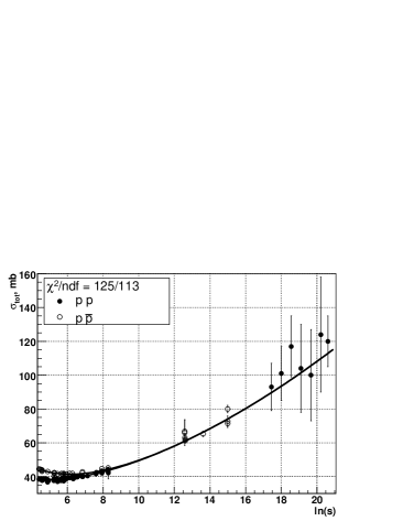
Figure 1: Fitting of total cross sections of $pp$ and $p\bar{p}$ collisions in LCNM

Having limited number of gluons we can describe the types of inelastic processes in proton-proton and proton-antiproton interactions.

III Three types of inelastic processes

From the obtained result of presence of only two gluons in initial state it follows existence of three types of inelastic processes in $pp$ and $p\bar{p}$ collisions.

There are three types of inelastic processes in proton-antiproton interaction. The first type is production of hadrons shower from decay of gluon string, it corresponds to constant contribution to total cross sections (Fig. 2a). The second type is shower produced from decay of two quark strings, it corresponds to contributions from one and two gluons (Fig. 2b). The third type is shower produced from decay of three quark strings, it corresponds to part of contribution from two gluons (Fig. 2c). In this case quark strings are produced between every quark of proton and antiquark of antiproton.

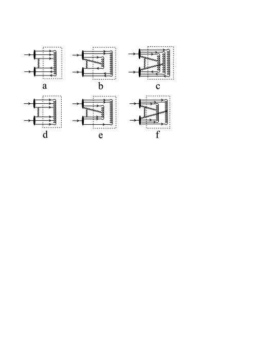
Figure 2: Types of inelastic processes for $p\bar{p}$ (a – c) and $pp$ interaction (d – f). Solid lines correspond to quarks and antiquarks, wavy lines to gluons, spirals to strings. Interaction in final state is marked by dashed block.

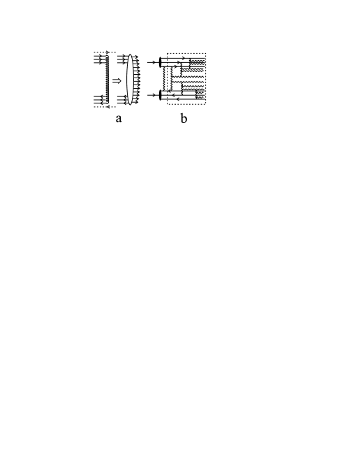
Figure 3: Hadrons production in gluon string. a) Amplitude of transition of two octet states produced after gluon exchange to hadrons, dashed lines show direction of octet states. b) One of possible diagrams of Fig. 2a; dashed block shows one of possible diagram of amplitude of transition of two octet states of Fig. 2a to hadrons

At the same time there are only two types of inelastic processes in proton-proton interaction, they are shower from gluon string (Fig. 2d) and shower from two quark strings (Fig. 2e,f). There are no three quark strings in $pp$ interaction because in this case strings can be formed between quark of one proton and diquark of another proton.

IV Multiplicity distributions for different processes

We suppose that hadrons multiplicity distribution in gluon string is normal distribution (Fig. 3).

Gluon pairs are sequentially produced in final state marked by dashed block. This production takes place until energy of pairs approaches hadrons mass. Then gluon pairs decays at several observable hadrons.

Every diagram of this type gives certain number of secondary hadrons. Number of such diagrams is considerably large. There is no suppression on energy because exchange is of vector type. Contributions from this diagrams have the same order of magnitude. So secondary hadrons multiplicity as random variable has to obey normal distribution because of central limit theorem of probability theory. Thus multiplicity distribution in gluon string is normal distribution.

We suppose that hadrons multiplicity distribution in quark string is negative binomial distribution (NBD). This is in good agreement with data on $e^{+}e^{-}$ annihilation at low energies where one quark string is produced with assurance. So multiplicity distribution in two quark strings is convolution of two NBD, namely NBD with double parameters, and in three quark strings it is convolution of three NBD, namely NBD with triple parameters.

Experimental charged multiplicities are normalized on non single diffraction cross sections, $\sigma_{nsd}=\sigma_{tot}-\sigma_{el}-\sigma_{sd}$. Pomeron contributions are the same as for total cross sections

$$\sigma^{nsd}_{vac}=\sigma_{0}^{nsd}(1+\delta_{1}^{nsd}\ln s+\delta_{2}^{nsd}\ln^{2}s),$$ (2)

here we divided formulae by constant term for convenience.

The fitting of vacuum contributions to non single diffraction cross sections is shown on Fig. 4, data were taken from bib4 ; bib5 . The value of $\chi^{2}$ to number of degrees of freedom 14 to 8 is caused by difference between data of UA4 and UA5 collaborations.

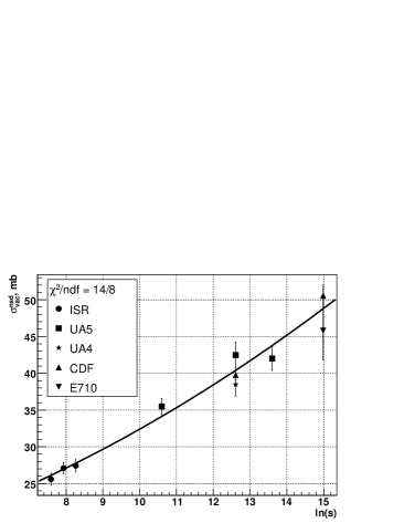
Figure 4: Vacuum contributions to non single diffraction cross sections of $pp$ and $p\bar{p}$ collisions

The obtained coefficients $\delta_{1}^{nsd}=0.075\pm 0.011$ and $\delta_{2}^{nsd}=0.007\pm 0.001$ determine the weights of configurations with gluon string, two quark strings, three quark strings.

Weight of normal distribution is defined by formulae (3) and it is the same for $pp$ and $p\bar{p}$ collisions.

$$\frac{1}{1+\delta_{1}^{nsd}\ln s+\delta_{2}^{nsd}(\ln s)^{2}}$$ (3)

Weights of double NBD are different for $pp$ (4) and $p\bar{p}$ (5) interactions because in case of proton-antiproton configuration with two gluons also gives contribution to three quark strings. It is taken into account by coefficient $c$, which does not depend on energy of collision.

$$\frac{\delta_{1}^{nsd}\ln s+\delta_{2}^{nsd}(\ln s)^{2}}{1+\delta_{1}^{nsd}\ln s+\delta_{2}^{nsd}(\ln s)^{2}}$$ (4)

$$\frac{\delta_{1}^{nsd}\ln s+(1-c)\,\delta_{2}^{nsd}(\ln s)^{2}}{1+\delta_{1}^{nsd}\ln s+\delta_{2}^{nsd}(\ln s)^{2}}$$ (5)

Therefore weight of triple NBD in configuration with three quark strings in $p\bar{p}$ collision is defined by formulae (6).

$$\frac{c\,\delta_{2}^{nsd}(\ln s)^{2}}{1+\delta_{1}^{nsd}\ln s+\delta_{2}^{nsd}(\ln s)^{2}}$$ (6)

But coefficient $c$ can not be evaluated from the existing data, so we consider two possible values of it – 0.25 and 0.75.

V Experimental data on charged multiplicity distributions

With assumptions stated in previous sections we described experimental data on charged particle multiplicity for $pp$ collisions at energy range from $\sqrt{s}=44.5$ to 200 GeV bib5 ; bib6 and for $p\bar{p}$ collisions from 200 to 1800 GeV bib7 – bib9 .

In case of $pp$ interaction weights of distributions are strictly defined by formulaes (3), (4). In Fig. 5 multiplicity distributions in $pp$ interaction at $\sqrt{s}=44.5$ and $\sqrt{s}=62.2$ GeV are shown. Here dash-dot line presents normal distribution in gluon string and dotted line presents double NBD in two quark strings, solid line is sum of these distributions.

Figure 5: $pp$ interaction at $\sqrt{s}=44.5$ ($\chi^{2}/ndf=13/15$) and $\sqrt{s}=62.2$ GeV ($\chi^{2}/ndf=13/16$)

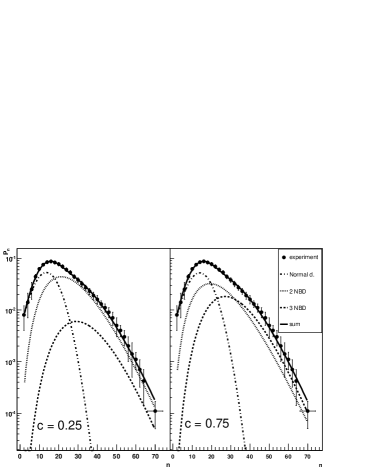
Figure 6: $p\bar{p}$ interaction at $\sqrt{s}=200$ GeV

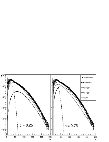
Figure 7: $p\bar{p}$ interaction at $\sqrt{s}=1800$ GeV

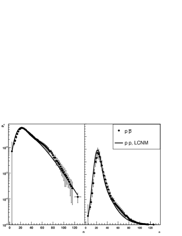
Figure 8: $p\bar{p}$ interaction at $\sqrt{s}=900$ GeV (points) and prediction for $pp$ at the same energy in LCNM for $c=0.75$ (line) in logarithmic and linear scale

But in case of $p\bar{p}$ interaction we have additional configuration with three quark strings, so weights of distributions are defined by formulaes (3), (5) and (6). The last two formulaes have undefined parameter – coefficient $c$ which describes appearance of three quark strings.

In Fig. 6 two fittings of $p\bar{p}$ collision at $\sqrt{s}=200$ GeV are shown. Here dash-dot line presents normal distribution in gluon string, dotted line presents double NBD in two quark strings and dashed line presents triple NBD in three quark strings, solid line is sum of these distributions. On the left side the case when 25 per cent of two gluons give three quark strings is shown, on the right side – the case when 75 per cent of two gluons give three quark strings. Values of $\chi^{2}$ to number of degrees of freedom are the same for both cases, $\chi^{2}/ndf=4/29$. As energy increases higher value of coefficient $c$ gives slightly better value of $\chi^{2}/ndf$, for example, at the highest available energy $\sqrt{s}=1800$ GeV $\chi^{2}/ndf=138/115$ when $c=0.25$ and $\chi^{2}/ndf=126/115$ when $c=0.75$ (Fig. 7).

After fitting all data we obtained energy dependence of parameters of gluon and quark strings ad thus we can predict the multiplicity distribution for $pp$ collisions at 900 GeV. This is the first high enough energy for which it will be possible to compare multiplicity distributions for $pp$ and $p\bar{p}$ interactions directly after start up of LHC. In the case of $c=0.25$ the shapes for both reactions are practically the same. But in the case of $c=0.75$ the systematic difference may be observed in region of “shoulder” given very precise measurements (Fig. 8).

VI Predictions for LHC energy 14 TeV

We predict the value of total cross section at $\sqrt{s}=14$ TeV to be

$$\sigma_{tot}^{pp}=101.30\pm 6.65.$$

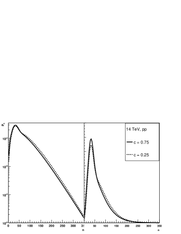
Figure 9: Prediction of multiplicity distribution for $pp$ interaction at $\sqrt{s}=14$ TeV in LCNM for $c=0.75$ (solid line) and for $c=0.25$ (dashed line) in logarithmic and linear scale

The multiplicity distribution for $pp$ interaction can be described as sum of normal distribution in gluon string and double negative binomial distribution in two quark strings. Weights of these distributions are strictly defined by formulaes (3), (4). Parameters of normal distribution are mean multiplicity in gluon string $\bar{n}_{gl}$ and standard deviation $\sigma_{gl}$. Parameters of double NBD are mean multiplicity in quark string $\bar{n}_{q}$ and shape parameter $k_{q}$. Since parameters of quark and gluon strings must be obtained at simultaneous fitting of $pp$ and $p\bar{p}$ distributions, they contain uncertainty of three quark strings coefficient $c$. So we have two sets of energy dependencies for gluon and quark string parameters.

$$\begin{array}[]{l}\underline{c=0.25}\\[2.84526pt] \bar{n}_{q}=3.45+0.46\ln^{2}\sqrt{s}\\[2.84526pt] k_{q}^{-1}=-0.24+0.11\ln\sqrt{s}\\[2.84526pt] \bar{n}_{gl}=-5.86+3.77\ln\sqrt{s}\\[2.84526pt] \sigma_{gl}=-2.67+1.52\ln\sqrt{s}\\[2.84526pt] \underline{c=0.75}\\[2.84526pt] \bar{n}_{q}=3.73+0.41\ln^{2}\sqrt{s}\\[2.84526pt] k_{q}^{-1}=-0.30+0.13\ln\sqrt{s}\\[2.84526pt] \bar{n}_{gl}=-6.65+3.97\ln\sqrt{s}\\[2.84526pt] \sigma_{gl}=-2.75+1.55\ln\sqrt{s}\end{array}$$

Predictions for charged multiplicity distribution for energy $\sqrt{s}=14$ TeV are shown in Fig. 9 for both cases of three quark strings coefficient $c$. The values of mean multiplicity are the following

$$\bar{n}_{pp}=\left\{\begin{array}[]{l}68.59\pm 4.47,\quad\mbox{if $c=0.25$;}\\ 63.20\pm 4.19,\quad\mbox{if $c=0.75$.}\end{array}\right.$$

It will be possible to distinguish between two values of coefficient $c$ when experimental data are available.

References

- (1) Abramovsky V.A., Kancheli O.V. (1980) JETP Letters 31:566-569, 32:498-501.
- (2) Cudell J.R. et al. (2000) Phys. Rev. D 61:034019.
- (3) Amsler C. et al. (2008) Phys. Lett. B 667:1-6.
- (4) Alner G.J. et al. (1986) Z. Phys. C 32:153-161.
- (5) Breakstone A. et al. (1984) Phys. Rev. D 30:528-535.
- (6) Sagerer J. (2004) http://www.phobos.bnl.gov/ Presentations/index.htm
- (7) Alner G.J. et al. (1987) Phys. Rept. 154:247-283.
- (8) Ansorge R.E. et al. (1989) Z. Phys. C 43:357-374.
- (9) Alexopoulos T. et al. (1998) Phys. Lett. B 435:453-457.