Diversity Order in ISI Channels with Single-Carrier Frequency-Domain Equalizers

Abstract

This paper analyzes the diversity gain achieved by single-carrier frequency-domain equalizer (SC-FDE) in frequency selective channels, and uncovers the interplay between diversity gain $d$, channel memory length $\nu$, transmission block length $L$, and the spectral efficiency $R$. We specifically show that for the class of minimum means-square error (MMSE) SC-FDE receivers, for rates $R\leq\log\frac{L}{\nu}$ full diversity of $d=\nu+1$ is achievable, while for higher rates the diversity is given by $d=\lfloor 2^{-R}L\rfloor+1$. In other words, the achievable diversity gain depends not only on the channel memory length, but also on the desired spectral efficiency and the transmission block length. A similar analysis reveals that for zero forcing SC-FDE, the diversity order is always one irrespective of channel memory length and spectral efficiency. These results are supported by simulations.

1 Introduction

A single-carrier frequency-domain equalizer (SC-FDE), as depicted in Fig. 1, consists of simple single-carrier block transmission with periodic cyclic-prefix insertion, and an equalizer that performs discrete Fourier Transform (DFT) and single-tap filtering followed by an inverse DFT (IDFT), where finally the equalizer output is fed into a slicer to make hard decisions on the input. Due to using computationally efficient fast Fourier transform, SC-FDE has lower complexity than time-domain equalizers. Structurally, SC-FDE has similarities with OFDM, but has the key distinction that SC-FDE decisions are made in the time domain, while OFDM decisions are made in the frequency domain. SC-FDE enjoys certain advantages over OFDM, as mentioned in, e.g., [1, 2]. In particular SC-FDE is not susceptible to the peak-to-average ratio (PAR) problem. Also, in OFDM one must code across frequency bands to capture frequency diversity, while in SC-FDE a similar issue does not exist since decisions are made in the time domain. In addition, SC-FDE has reduced sensitivity to carrier frequency errors, and confines the frequency-domain processing to the receiver. SC-FDE is deemed promising for broadband wireless communication [1, 3, 4, 2] and has been proposed for implementation in the 3GPP long term evolution (LTE) standard. This paper analyzes the SC-FDE and unveils hitherto unknown relationships between its diversity, spectral efficiency, and transmission block length. The explicit dependence of diversity on the transmission block length is especially intriguing, and to the best of our knowledge has no parallel in the literature of equalizers for dispersive channels.

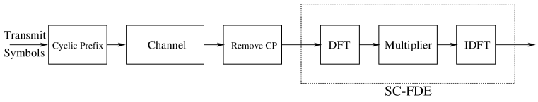
Figure 1: Block diagram of a SC-FDE system.

We start by briefly reviewing some of the existing results on the diversity gain of various block transmission schemes. It is known that uncoded OFDM is vulnerable to weak symbol detection when the frequency selective channel has nulls on the DFT grid, and therefore, uncoded OFDM may not capture the full diversity of the inter-symbol interference (ISI) channel [6]. To mitigate this effect, various coded-OFDM schemes have been considered [7, 8]. Motivated to achieve full diversity without error-control coding, complex-field coded (CFC)-OFDM has been introduced [6], where it is shown to achieve full diversity with maximum likelihood (ML) detection. CFC-OFDM achieves its diversity in a manner essentially similar to the so-called signal space diversity of Boutros and Viterbo [9], by sending linear combinations of the uncoded symbols via each subcarrier. It has been shown that both zero-padded single-carrier block transmission and cyclic-prefix single-carrier block transmission are special cases of CFC-OFDM [6]; therefore, by deploying ML detection, they also achieve full diversity.

The complexity of ML detection motivates the study of linear equalizers. The first analysis on the diversity order of CFC-OFDM with linear equalization was provided in [10], where it is shown that with additional constraints on the code design, zero-forcing (ZF) linear block equalizers can achieve the same diversity order as ML detection. Furthermore, in [11] it has been shown that zero-padded single-carrier block transmission, as a special case of CFC-OFDM, meets the conditions discussed in [10] and therefore achieves full diversity by exploiting ZF equalization.

Although it has been established that a cyclic-prefix single-carrier block transmission with ML detection, achieves full diversity [6], the result clearly cannot be applied to SC-FDE, because SC-FDE does not yield ML decisions. Furthermore the linear equalization results mentioned in [10, 11] do not apply to SC-FDE either, since SC-FDE does not satisfy the conditions in [10, 11]. This distinction is further solidified in the sequel where we show that SC-FDE in fact does not enjoy unconditional full diversity.

Our analyses reveal that for minimum-mean-square-error (MMSE) SC-FDE the diversity order varies between 1 and channel length, $\nu+1$, depending on the transmission setup. We demonstrate a tradeoff between the achievable diversity order, data transmission rate, $R$ (bits/second/Hz), channel memory length, $\nu$, and transmission block length, $L$. Specifically, at rates lower than $\log\frac{L}{\nu}$, full diversity of $\nu+1$ is achieved, while at higher rates, the diversity gain is $\lfloor 2^{-R}L\rfloor+1$. These results support the earlier analysis in [12, 13], where it has been shown that for very low and very high data rates, diversity gains 1 and $\nu+1$ are achieved, respectively. We also investigate the diversity order of zero-forcing (ZF) SC-FDE and find that the achievable diversity order is always 1, which is similar to that of OFDM with zero-forcing equalization [14].

The rest of this paper is organized as follows. In Section 2 the system model and some definitions are provided. Diversity analysis for MMSE-SC-FDE and ZF-SC-FDE are provided in sections 3 and 4, respectively. Section 5 provides numerical evaluations and simulation results and concluding remarks are presented in Section 6.

2 System Description

2.1 SC-FDE vs. OFDM

As seen in the baseband model of SC-FDE (Fig. 1), after removing the cyclic-prefix, a DFT operator is applied to the received signal, each sample is multiplied by a complex coefficient and then an IDFT transforms the signal back to the time domain. In the time domain, the equalizer output is fed into a slicer to make hard decisions on the transmitted vector.

In OFDM both channel equalization and detection are performed in the frequency domain, whereas in SC-FDE, while channel equalization is done in the frequency domain, receiver decisions are made in the time domain, which leads to differences in the performance of OFDM vs. SC-FDE. The underlying reason for such performance difference is that in uncoded OFDM, the subcarriers suffering from deep fade will exhibit poor performance. On the other hand, in SC-FDE detection decisions are made based on the (weighted) average performance of subcarriers, which is expected to be more robust to the fading of individual subcarriers. For more discussions see [1, 4].

2.2 Transmission Model

We consider a frequency selective quasi-static wireless fading channel with memory length $\nu$,

$$H(z)=h_{0}+h_{1}z^{-1}+\cdots+h_{\nu}z^{-\nu}.$$

The channel follows a block fading model where the channel coefficients are independent complex Gaussian $\mathcal{CN}(0,1)$ random variables that remain unchanged over the transmission block of length $L$, and change to an independent state afterwards. Received signals are contaminated with zero-mean unit variance complex additive white Gaussian noise (AWGN). The channel output is given by

$$\boldsymbol{y}=\sqrt{{{\sf SNR}}}\boldsymbol{H}\boldsymbol{x}+\boldsymbol{n},$$ (1)

where $\boldsymbol{x}=[x(L),\dots,x(-\nu+1)]^{T}$ denotes the transmitted block and $\boldsymbol{y}=[y(L),\dots,y(1)]^{T}$ is the vector of received symbols before equalization. We normalize $\boldsymbol{x}$ such that the average transmit power for each entry of $\boldsymbol{x}$ is 1, and ${{\sf SNR}}$ accounts for the average signal-to-noise ratio (${{\sf SNR}}$) at the transmitter. Channel noise is denoted by $\boldsymbol{n}=[n(L),\dots,n(1)]^{T}$, and the channel matrix is represented by

$$\boldsymbol{H}_{L\times(L+\nu)}\stackrel{{\scriptstyle\scriptscriptstyle\triangle}}{{=}}\begin{bmatrix}h_{0}&h_{1}&\cdots&h_{\nu}&0&\cdots&0\\ 0&h_{0}&h_{1}&\cdots&h_{\nu}&\cdots&0\\ \vdots&\ddots&\ddots&\ddots&\ddots&\ddots&\vdots\\ 0&\cdots&0&h_{0}&h_{1}&\cdots&h_{\nu}\end{bmatrix}.$$ (2)

To remove inter-block interference, a cyclic prefix is inserted at the beginning of each transmit block, giving rise to the equivalent channel

$$\boldsymbol{H}_{\rm{eq}}\stackrel{{\scriptstyle\scriptscriptstyle\triangle}}{{=}}\begin{bmatrix}h_{0}&h_{1}&\cdots&h_{\nu-1}&h_{\nu}&0&\cdots&0\\ 0&h_{0}&h_{1}&\cdots&h_{\nu-1}&h_{\nu}&\cdots&0\\ \vdots&\vdots&\vdots&\vdots&\vdots&\vdots&&\vdots\\ h_{1}&h_{2}&\cdots&h_{\nu}&0&0&\cdots&h_{0}\end{bmatrix}.$$

This $L\times L$ circulant matrix $\boldsymbol{H}_{\rm{eq}}$ has eigen decomposition $\boldsymbol{H}_{\rm{eq}}=\boldsymbol{Q}^{H}\boldsymbol{\Lambda}\boldsymbol{Q}$, where $\boldsymbol{Q}$ is the discrete Fourier transform (DFT) matrix with elements

$$\boldsymbol{Q}(m,n)=\frac{1}{\sqrt{L}}\exp\bigg{[}-j\frac{2\pi}{L}(m-1)(n-1)\bigg{]},\quad\mbox{for}\;\;m,n=1,\dots,L,$$

where we have $\boldsymbol{Q}^{H}\boldsymbol{Q}=\boldsymbol{I}$. Also, the diagonal matrix $\boldsymbol{\Lambda}$ contains the $L$-point (non-unitary) DFT of the first row of $\boldsymbol{H}_{\rm{eq}}$ given by

$$\lambda_{k}\stackrel{{\scriptstyle\scriptscriptstyle\triangle}}{{=}}\boldsymbol{\Lambda}_{k,k}=\sum_{i=0}^{\nu}h_{i}e^{-j\frac{2i\pi(k-1)}{L}},\quad\mbox{for}\;\;k=1,\dots,L.$$ (3)

Each eigenvalue $\lambda_{k}$ is a linear combination of channel coefficients, which are zero mean complex Gaussian random variables. Therefore $\{\lambda_{k}\}_{k=1}^{L}$ also have zero mean complex Gaussian distribution.

Remark 1

For the special case of $L=\nu+1$, the eigenvalues $\{\lambda_{k}\}_{k=1}^{L}$ are independent random variables.

We assume that the received signal is processed by a SC-FDE, designated by $\boldsymbol{W}$, where its output $\tilde{\boldsymbol{y}}\stackrel{{\scriptstyle\scriptscriptstyle\triangle}}{{=}}[\tilde{y}(L),\dots,\tilde{y}(1)]$ is

$$\tilde{\boldsymbol{y}}\stackrel{{\scriptstyle\scriptscriptstyle\triangle}}{{=}}\boldsymbol{W}\boldsymbol{y}=\sqrt{{{\sf SNR}}}\boldsymbol{W}\boldsymbol{H}_{\rm eq}\boldsymbol{x}+\boldsymbol{W}\boldsymbol{n}.$$

Throughout the paper we denote the transmission signal-to-noise ratio by ${{\sf SNR}}$ and we say that the two functions $f({{\sf SNR}})$ and $g({{\sf SNR}}$) are exponentially equal, denoted by $f({{\sf SNR}}){\overset{\text{\Large.}}{=}}g({{\sf SNR}})$, when

$$\lim_{{{\sf SNR}}\rightarrow\infty}\frac{\log f({{\sf SNR}})}{\log{{\sf SNR}}}=\lim_{{{\sf SNR}}\rightarrow\infty}\frac{\log g({{\sf SNR}})}{\log{{\sf SNR}}}.$$

The ordering operators $\;{\overset{\text{\Large.}}{\leq}}\;$ and $\;{\overset{\text{\Large.}}{\geq}}\;$ are also defined accordingly. If $f({{\sf SNR}}){\overset{\text{\Large.}}{=}}{{\sf SNR}}^{d}$, we say that $d$ is the exponential order of $f({{\sf SNR}})$.

2.3 Diversity Analysis

The diversity gain describes how fast the average pairwise error probability decays as the ${{\sf SNR}}$ increases. For an ISI channel with memory length $\nu$ and SC-FDE receiver with block length $L$, we denote the diversity gain at data rate $R$ by ${d(R,\nu,L)}$ and is given by

$${d(R,\nu,L)}\stackrel{{\scriptstyle\scriptscriptstyle\triangle}}{{=}}-\lim_{{{\sf SNR}}\rightarrow\infty}\frac{\log P_{\rm err}(R,\nu,L)}{\log{{\sf SNR}}},$$ (4)

where $P_{\rm err}(R,\nu,L)$ denotes the average pairwise error probability, which is the probability that the receiver decides erroneously in favor of $s_{k}$, while $s_{j}$ was transmitted, i.e.,

$$P_{\rm err}(R,\nu,L)\stackrel{{\scriptstyle\scriptscriptstyle\triangle}}{{=}}{\mathbb{E}}\bigg{\{}P\big{[}s_{j}\rightarrow s_{k}\;|\boldsymbol{H}=H\big{]}\bigg{\}}={\mathbb{E}}\bigg{\{}P\Big{[}\|\tilde{y}(\ell)-\sqrt{{{\sf SNR}}}s_{j}\|>\|\tilde{y}(\ell)-\sqrt{{{\sf SNR}}}s_{k}\;\big{|}\boldsymbol{H}=H\Big{]}\bigg{\}}.$$

In this paper we aim to characterize ${d(R,\nu,L)}$, whose direct analysis requires a PEP analysis that depends on the choice of signaling. This approach is not easily tractable and as a remedy, we first turn to mutual information and outage analysis and characterize the exponential order of the outage probability. In the next step, by establishing that the outage probability and the average PEP exhibit identical exponential orders, we can characterize ${d(R,\nu,L)}$.

Therefore, we will also perform outage analysis for SC-FDE, whose related definitions are as follows. Due to the equalizer structure, the effective mutual information between $\boldsymbol{x}$ and $\tilde{\boldsymbol{y}}$ is equal to the sum of the mutual information of their components (sub-streams) [15]

$${I}(\boldsymbol{x};\tilde{\boldsymbol{y}})=\frac{1}{L}\sum_{\ell=1}^{L}{I}(x_{\ell};\tilde{y}_{\ell}).$$ (5)

Subsequently, we define the following outage-type quantities

$$P_{\rm out}(R,\nu,L) \stackrel{{\scriptstyle\scriptscriptstyle\triangle}}{{=}} P\big{[}{I}(\boldsymbol{x};\tilde{\boldsymbol{y}})<R\big{]},$$

$$\mbox{and}\quad{d_{\rm out}(R,\nu,L)} \stackrel{{\scriptstyle\scriptscriptstyle\triangle}}{{=}} -\lim_{{{\sf SNR}}\rightarrow\infty}\frac{\log P_{\rm out}(R,\nu,L)}{\log{{\sf SNR}}}.$$ (6)

3 Diversity Analysis of MMSE SC-FDE

We start with finding the unbiased decision-point ${\sf SINR}$. For the transmission model given in (1) the MMSE linear equalizer is

$$\boldsymbol{W}_{\rm MMSE}=\big{[}\boldsymbol{H}_{\rm eq}^{H}\boldsymbol{H}_{\rm eq}+{{\sf SNR}}^{-1}\boldsymbol{I}\big{]}^{-1}\boldsymbol{H}_{\rm eq}^{H},$$ (7)

and the output of the equalizer can be found as

$$\tilde{\boldsymbol{y}}=\big{[}\boldsymbol{H}_{\rm eq}^{H}\boldsymbol{H}_{\rm eq}+{{\sf SNR}}^{-1}\boldsymbol{I}\big{]}^{-1}\boldsymbol{H}_{\rm eq}^{H}\boldsymbol{H}_{\rm eq}\boldsymbol{x}+\big{[}\boldsymbol{H}_{\rm eq}^{H}\boldsymbol{H}_{\rm eq}+{{\sf SNR}}^{-1}\boldsymbol{I}\big{]}^{-1}\boldsymbol{H}_{\rm eq}^{H}\boldsymbol{n}.$$

We also define the noise term $\tilde{\boldsymbol{n}}\stackrel{{\scriptstyle\scriptscriptstyle\triangle}}{{=}}[\tilde{n}(L),\dots,\tilde{n}(1)]$ as

$$\tilde{\boldsymbol{n}}\stackrel{{\scriptstyle\scriptscriptstyle\triangle}}{{=}}\tilde{\boldsymbol{y}}-\sqrt{{{\sf SNR}}}\boldsymbol{x}=\sqrt{{{\sf SNR}}}(\boldsymbol{W}\boldsymbol{H}_{\rm eq}-\boldsymbol{I})\boldsymbol{x}+\boldsymbol{W}\boldsymbol{n},$$ (8)

which accounts for the combined effect of the channel noise $\boldsymbol{n}$ and the ISI residual due to MMSE interference suppression. By recalling the eigen decomposition of $\boldsymbol{H}_{\rm eq}$ and noting that $\mathbb{E}[\boldsymbol{n}]=\boldsymbol{0},\;\mathbb{E}[\boldsymbol{n}\boldsymbol{n}^{H}]=\boldsymbol{I}$, some simple manipulations provide that

$$\boldsymbol{\mu}_{\tilde{\boldsymbol{n}}} \stackrel{{\scriptstyle\scriptscriptstyle\triangle}}{{=}} \mathbb{E}[\tilde{\boldsymbol{n}}]=\sqrt{{{\sf SNR}}}(\boldsymbol{W}\boldsymbol{H}_{\rm eq}-\boldsymbol{I})\boldsymbol{x},$$ (9)

$$\mbox{and}\quad\qquad\boldsymbol{R}_{\tilde{\boldsymbol{n}}} \stackrel{{\scriptstyle\scriptscriptstyle\triangle}}{{=}} \mathbb{E}[\tilde{\boldsymbol{n}}\tilde{\boldsymbol{n}}^{H}]=\big{[}\boldsymbol{H}_{\rm eq}^{H}\boldsymbol{H}_{\rm eq}+{{\sf SNR}}^{-1}\boldsymbol{I}\big{]}^{-1}.$$ (10)

Due to the underlying symmetry, it can be show that the diagonal elements of $\boldsymbol{R}_{\tilde{\boldsymbol{n}}}$ are identical. Therefore, the unbiased decision-point ${\sf SINR}$ of MMSE SC-FDE for detecting symbol $x(\ell),1\leq\ell\leq L$ (or the $\ell^{th}$ information stream) is

$$\gamma_{\ell}^{\rm MMSE} \stackrel{{\scriptstyle\scriptscriptstyle\triangle}}{{=}} \frac{{{\sf SNR}}}{\boldsymbol{R}_{\tilde{\boldsymbol{n}}}(\ell,\ell)}-1=\frac{{{\sf SNR}}}{\frac{1}{L}{\rm tr}[\boldsymbol{R}_{\tilde{\boldsymbol{n}}}]}-1=\frac{{{\sf SNR}}}{\frac{1}{L}{\rm tr}\big{[}\boldsymbol{H}_{\rm eq}^{H}\boldsymbol{H}_{\rm eq}+{{\sf SNR}}^{-1}\boldsymbol{I}\big{]}^{-1}}-1$$ (11)

$$= \frac{1}{\frac{1}{L}{\rm tr}\big{[}{{\sf SNR}}\;\boldsymbol{\Lambda}\boldsymbol{\Lambda}^{H}+\boldsymbol{I}\big{]}^{-1}}-1=\bigg{[}\frac{1}{L}\sum_{k=1}^{L}\frac{1}{1+{{\sf SNR}}|\lambda_{k}|^{2}}\bigg{]}^{-1}-1,$$

which does not depend on $\ell$ and is identical for all information streams. Therefore, the mutual information in (5) becomes

$${I}_{\rm MMSE}(\boldsymbol{x};\tilde{\boldsymbol{y}})=\frac{1}{L}\sum_{\ell=1}^{L}\log(1+\gamma_{\ell}^{\rm MMSE})=-\log\bigg{[}\frac{1}{L}\sum_{\ell=1}^{L}\frac{1}{{{\sf SNR}}|\lambda_{k}|^{2}+1}\bigg{]},$$ (12)

and the outage probability for the target rate $R$, which is the probability that the mutual information ${I}(\boldsymbol{x};\tilde{\boldsymbol{y}})$ falls below $R$ is

$$P_{\rm out}(R,\nu,L)=P\bigg{[}\frac{1}{L}\sum_{k=1}^{L}\frac{1}{1+{{\sf SNR}}|\lambda_{k}|^{2}}>2^{-R}\bigg{]}.$$ (13)

3.1 Outage Analysis

For analyzing the outage probability, we start with the special case of $L=\nu+1$, and then generalize the result for the arbitrary choices of $L$. The following lemma has a key role in finding the exponential order of the outage probability.

Lemma 1

For $n$ i.i.d. normal complex Gaussian random variables $\{\lambda_{k}\}_{k=1}^{n}$ and a real-valued constant $m\in(0,n)$ we have

$$P\bigg{[}\sum_{k=1}^{n}\frac{1}{1+{{\sf SNR}}|\lambda_{k}|^{2}}>m\bigg{]}{\overset{\text{\Large.}}{=}}{{\sf SNR}}^{-(\lfloor m\rfloor+1)},$$ (14)

where $\lfloor\cdot\rfloor$ denotes the floor function.

Proof: We define

$$\alpha_{k}\stackrel{{\scriptstyle\scriptscriptstyle\triangle}}{{=}}-\frac{\log|\lambda_{k}|^{2}}{\log{{\sf SNR}}},\quad\mbox{for}\;\;k=1,\dots,n\;\;,$$ (15)

based on which we can write the equality-in-the-limit

$$\frac{1}{1+{{\sf SNR}}|\lambda_{k}|^{2}}\;{\overset{\text{\Large.}}{=}}\begin{cases}{{\sf SNR}}^{\alpha_{k}-1}&\alpha_{k}<1\\ 1&\alpha_{k}>1\end{cases}\;\;.$$

This indicates that the term $\frac{1}{1+{{\sf SNR}}|\lambda_{k}|^{2}}$ is either 0 or 1 corresponding to the regions $\alpha_{k}<1$ and $\alpha_{k}>1$, respectively. Therefore, the probability in (14) is exponentially equal to having at least $(\lfloor m\rfloor+1)$ number of $\{\alpha_{k}\}$ greater 1. In other words,

$$\sum_{k=1}^{n}\frac{1}{1+{{\sf SNR}}|\lambda_{k}|^{2}} {\overset{\text{\Large.}}{=}} \sum_{\alpha_{k}>1}1+\sum_{\alpha_{k}<1}{{\sf SNR}}^{\alpha_{k}-1}{\overset{\text{\Large.}}{=}}M(\boldsymbol{\alpha})+\max_{\{\alpha_{k}\;|\;\alpha_{k}<1\}}{{\sf SNR}}^{\alpha_{k}-1},$$ (16)

where we have defined $\boldsymbol{\alpha}\stackrel{{\scriptstyle\scriptscriptstyle\triangle}}{{=}}[\alpha_{1},\dots,\alpha_{n}]$ and a new random variable

$$M(\boldsymbol{\alpha})\stackrel{{\scriptstyle\scriptscriptstyle\triangle}}{{=}}\sum_{\alpha_{k}>1}1\;,$$ (17)

i.e., $M(\boldsymbol{\alpha})$ counts the number of $\alpha_{k}>1$. Clearly $\{\alpha_{1},\ldots,\alpha_{n}\}$ and $M(\boldsymbol{\alpha})$ are random variables induced by $\{\lambda_{1},\ldots,\lambda_{n}\}$. Knowing that $|\lambda_{k}|^{2}$ has exponential distribution, by using arguments similar to [5] it can be verified that the cumulative density function (CDF) of $\alpha_{k}$ is

$$F_{\alpha_{k}}(\alpha){\overset{\text{\Large.}}{=}}\exp\big{(}-{{\sf SNR}}^{-\alpha}\big{)}.$$ (18)

As a result $P(\alpha_{k}>1){\overset{\text{\Large.}}{=}}1-\exp(-{{\sf SNR}}^{-1}){\overset{\text{\Large.}}{=}}{{\sf SNR}}^{-1}$. Invoking the independence of $\{\lambda_{k}\}$, and thereof the independence of $\{\alpha_{k}\}$, provides that the random variable $M(\boldsymbol{\alpha})$ is binomially distributed and its binomial parameter is asymptotically ${{\sf SNR}}^{-1}$. Hence,

$$P\bigg{[}\sum_{k=1}^{n}\frac{1}{1+{{\sf SNR}}|\lambda_{k}|^{2}}>m\bigg{]} {\overset{\text{\Large.}}{=}} P\big{(}M(\boldsymbol{\alpha})+\max_{\{\alpha_{k}\;|\;\alpha_{k}<1\}}{{\sf SNR}}^{\alpha_{k}-1}>m\big{)}$$

$${\overset{\text{\Large.}}{=}} P(M(\boldsymbol{\alpha})>m)$$

$$= \sum_{i=\lfloor m\rfloor+1}^{n}P\big{(}M(\boldsymbol{\alpha})=i\big{)}$$

$${\overset{\text{\Large.}}{=}} \sum_{i=\lfloor m\rfloor+1}^{n}{n\choose i}{{\sf SNR}}^{-i}\underset{{\overset{\text{\Large.}}{=}}1}{\underbrace{\big{(}1-{{\sf SNR}}^{-1}\big{)}}}^{n-i}$$

$${\overset{\text{\Large.}}{=}} {{\sf SNR}}^{-(\lfloor m\rfloor+1)},$$

In the above equations, the first (asymptotic) equality follows from exchange of limit and probability due to continuity of functions, the second equality holds because $\max_{\{\alpha_{k}\;|\;\alpha_{k}<1\}}{{\sf SNR}}^{\alpha_{k}-1}$ diminishes at high ${{\sf SNR}}$, and the final equality follows from the fact that inside the summation the term with the largest exponent dominates. This concludes the proof of the lemma.   

Now, by using the above lemma, we offer the following theorem which establishes the exponential order of the outage probability for $L=\nu+1$.

Theorem 1 (Outage Probability for $L=\nu+1$)

In an ISI channel with memory length $\nu$, transmission block length $L=\nu+1$, data rate $R$, and an MMSE SC-FDE receiver, the outage probability satisfies

$$P_{\rm out}(R,\nu,\nu+1){\overset{\text{\Large.}}{=}}{{\sf SNR}}^{-d_{\rm out}(R,\nu,\nu+1)},$$

where

$$d_{\rm out}(R,\nu,\nu+1)=\lfloor 2^{-R}(\nu+1)\rfloor+1.$$ (19)

Proof: Given the mutual information in (12), for the case of $L=\nu+1$ the outage probability is

$$P_{\rm out}(R,\nu,\nu+1) = P\big{[}{I}_{\rm MMSE}(\boldsymbol{x};\tilde{\boldsymbol{y}})<R\big{]}=P\bigg{[}\sum_{k=1}^{\nu+1}\frac{1}{1+{{\sf SNR}}|\lambda_{k}|^{2}}>2^{-R}(\nu+1)\bigg{]}.$$ (20)

As mentioned earlier in Remark 1 for $L=\nu+1$, $\{\lambda_{k}\}$ are i.i.d. with complex Gaussian distribution. By setting $n=\nu+1$ and $m\stackrel{{\scriptstyle\scriptscriptstyle\triangle}}{{=}}2^{-R}(\nu+1)$ for nonzero rates $R>0$, it is seen that $m\in(0,\nu+1)$. Therefore, the necessary conditions of Lemma 1 are satisfied and consequently we have

$$P_{\rm out}(R,\nu,\nu+1){\overset{\text{\Large.}}{=}}{{\sf SNR}}^{-(\lfloor 2^{-R}(\nu+1)\rfloor+1)},$$ (21)

which concludes the proof.   

In the next step, we generalize the results above for the arbitrary choice of block length $L$. We offer the following lemma which facilitates the transition from the special case of $L=\nu+1$ to any the arbitrary value for $L$.

Lemma 2

Consider the vector of channel coefficients $\boldsymbol{h}\stackrel{{\scriptstyle\scriptscriptstyle\triangle}}{{=}}[h_{0},\dots,h_{\nu}]$ together with its two zero-padded versions $\boldsymbol{g}_{1\times L}$ and $\boldsymbol{g}^{\prime}_{1\times L^{\prime}}$ that differ only in the number of zeros padded, i.e.,

$$\boldsymbol{g}_{1\times L}\stackrel{{\scriptstyle\scriptscriptstyle\triangle}}{{=}}[h_{0},\dots,h_{\nu},\underset{L-\nu-1}{\underbrace{0,\dots,0}}],\qquad\mbox{and}\qquad\boldsymbol{g}^{\prime}_{1\times L^{\prime}}\stackrel{{\scriptstyle\scriptscriptstyle\triangle}}{{=}}[h_{0},\dots,h_{\nu},\underset{L^{\prime}-\nu-1}{\underbrace{0,\dots,0}}].$$

The DFT vectors $\{\lambda_{i}\}_{1\times L}\stackrel{{\scriptstyle\scriptscriptstyle\triangle}}{{=}}{\rm DFT}(\boldsymbol{g})$ and $\{\lambda^{\prime}_{i}\}_{1\times L^{\prime}}\stackrel{{\scriptstyle\scriptscriptstyle\triangle}}{{=}}{\rm DFT}(\boldsymbol{g}^{\prime})$ have the following property for any real-valued constant $m\in(0,\nu+1)$

$$P\bigg{[}\sum_{k=1}^{L}\frac{1}{1+{{\sf SNR}}|\lambda_{k}|^{2}}>m\bigg{]}{\overset{\text{\Large.}}{=}}P\bigg{[}\sum_{k=1}^{L^{\prime}}\frac{1}{1+{{\sf SNR}}|\lambda^{\prime}_{k}|^{2}}>m\bigg{]}.$$ (22)

Proof: See Appendix A.   

By using the above lemma, we generalize $d_{\rm out}(R,\nu,\nu+1)$ as characterized in Theorem 1 for the general case of arbitrary $L$ to obtain ${d_{\rm out}(R,\nu,L)}$. The result offered in the next theorem demonstrates how altering the transmission block length from $L$ to $L^{\prime}$ influences the characterization of ${d_{\rm out}(R,\nu,L)}$.

Theorem 2

In an ISI channel with memory length $\nu$ and MMSE SC-FDE receiver, the exponential order of the outage probability of block transmission length $L$ and rate $R$ is equivalent to that of block length $L^{\prime}$ and rate $R+\log\frac{L^{\prime}}{L}$, i.e.,

$${d_{\rm out}(R,\nu,L)}=d_{\rm out}\big{(}R+\log\frac{L^{\prime}}{L},\nu,L^{\prime}\big{)}.$$ (23)

Proof: By defining $\beta=\log\frac{L^{\prime}}{L}$ we have

$$P_{\rm out}(R,\nu,L) = P\bigg{[}\frac{1}{L}\sum_{k=1}^{L}\frac{1}{1+{{\sf SNR}}|\lambda_{k}|^{2}}>2^{-R}\bigg{]}$$

$$= P\bigg{[}\sum_{k=1}^{L}\frac{1}{1+{{\sf SNR}}|\lambda_{k}|^{2}}>L2^{-R}\bigg{]}$$

$${\overset{\text{\Large.}}{=}} P\bigg{[}\sum_{k=1}^{L^{\prime}}\frac{1}{1+{{\sf SNR}}|\lambda^{\prime}_{k}|^{2}}>L2^{-R}\bigg{]}$$

$$= P\bigg{[}\frac{1}{L^{\prime}}\sum_{k=1}^{L^{\prime}}\frac{1}{1+{{\sf SNR}}|\lambda^{\prime}_{k}|^{2}}>\frac{L}{L^{\prime}}2^{-R}\bigg{]}$$

$$= P\bigg{[}\frac{1}{L^{\prime}}\sum_{k=1}^{L^{\prime}}\frac{1}{1+{{\sf SNR}}|\lambda^{\prime}_{k}|^{2}}>2^{-(\beta+R)}\bigg{]}$$

$$= P_{\rm out}\big{(}R+\beta,\nu,L^{\prime}\big{)},$$ (26)

where (3.1) holds according to Lemma (2) for $m=L2^{-R}$. Exponential equality of  (3.1) and (26) shows that

$${{\sf SNR}}^{-d_{\rm out}(R,\nu,L)}{\overset{\text{\Large.}}{=}}{{\sf SNR}}^{-d_{\rm out}(R+\log\frac{L^{\prime}}{L},\nu,L^{\prime})},$$

which completes the proof.   

Combining Theorem 1 and Theorem 2 leads to the main result of this paper as stated in the following corollary.

Corollary 1 (Outage Probability)

In an ISI channel with memory length $\nu$, transmission block length $L$, data rate $R$, and an MMSE SC-FDE receiver, the outage probability is characterized by

$$P_{\rm out}(R,\nu,L){\overset{\text{\Large.}}{=}}{{\sf SNR}}^{-{d_{\rm out}(R,\nu,L)}},$$

where,

$${d_{\rm out}(R,\nu,L)}=\begin{cases}\nu+1&\mbox{\rm for}\;R\leq\log\frac{L}{\nu}\\ \lfloor 2^{-R}L\rfloor+1&\mbox{\rm for}\;R>\log\frac{L}{\nu}\end{cases}.$$ (27)

Proof: We use the result of the case $L=\nu+1$ as the benchmark. For this case as given in (19) we observe that for the rate interval $(\log\frac{\nu+1}{i},\log\frac{\nu+1}{i-1}]$, we have $d_{\rm out}=i$, for $i=1,\dots,\nu+1$. By invoking the result of Theorem 2 and setting $L^{\prime}=\nu+1$ it is concluded that for block transmission length $L$, the rate interval for which ${d_{\rm out}(R,\nu,L)}=1$ shifts to the interval $(0,\log\frac{L}{\nu}]$ and the rate interval for which ${d_{\rm out}(R,\nu,L)}=i\geq 2$ shifts to the interval $(\log\frac{\nu+1}{i}+\log\frac{L}{\nu+1},\log\frac{\nu+1}{i-1}+\log\frac{L}{\nu+1}]=(\log\frac{L}{i},\log\frac{L}{i-1}]$ for $i=2,\dots,\nu+1$. Such intervals can be mathematically represented as in (27).   

The analyses above convey that the maximum value of ${d_{\rm out}(R,\nu,L)}$ is $\nu+1$ and is achievable for all rates not exceeding $\log\frac{L}{\nu}$. If transmission rate increases beyond this point, ${d_{\rm out}(R,\nu,L)}$ degrades following the rule given in (27). Such degradation can be compensated by increasing $L$.

3.2 PEP Analysis

In this section, we find lower and upper bounds on ${d(R,\nu,L)}$ and show that these bounds meet and are equal to ${d_{\rm out}(R,\nu,L)}$. The result is established via two lemmas. We start by a lemma that utilizes the techniques developed in [5, Lemma 5]. This lemma differs with [5, Lemma 5] in the sense that we are dealing with rate, whereas [5, Lemma 5] deals with multiplexing gain, and also the analysis of [5, Lemma 5] exploits the fact that outage probability is continuous with respect to multiplexing gain, while in our analysis, as shown in Corollary 1, the outage probability is only left-continuous with respect to rate.

Lemma 3 (Upper bound)

For an ISI channel with MMSE SC-FDE receiver we have

$${d_{\rm out}(R,\nu,L)}\geq{d(R,\nu,L)}$$

if $\exists\;d_{\min},\;d_{\max}\in\mathbb{R}_{++}$ such that $d_{\min}\leq{d(R,\nu,L)}\leq d_{\max}$.

Proof: We fix a codebook $\mathcal{C}$ of size $2^{Rl}$, where $R$ and $l$ are data rate and code length, respectively and $\boldsymbol{x}\in\mathcal{C}$ is the input to the system. The system input and output are related through the mapping $\tilde{\boldsymbol{y}}=\boldsymbol{f}(\boldsymbol{x})+\tilde{\boldsymbol{n}}$, where $\boldsymbol{f}$ accounts for the combined effect channel and equalizer. All transmit messages are assumed to be equiprobable which provides ${\cal H}(\boldsymbol{x})=\log|{\cal C}|=Rl$, where ${\cal H}(\cdot)$ denotes entropy. By defining $E$ as the error event from Fano’s inequality we get [16, 2.130]

$${\cal H}(P(E)\;|\;\boldsymbol{f}=f)+Rl\times P(E\;|\;\boldsymbol{f}=f)\geq{\cal H}(\boldsymbol{x}\;|\;\tilde{\boldsymbol{y}},\;\boldsymbol{f}=f).$$

Therefore,

$$P({E}\;|\;\boldsymbol{f}=f)\geq\frac{Rl-{I}(\boldsymbol{x};\tilde{\boldsymbol{y}}\;|\;\boldsymbol{f}=f)}{Rl}-\frac{\mathcal{H}(P(E)\;|\;\boldsymbol{f}=f)}{Rl}.$$ (28)

By defining $D_{\delta}$ for any value of $\delta>0$ as

$$\mathcal{D}_{\delta}\stackrel{{\scriptstyle\scriptscriptstyle\triangle}}{{=}}\{f:{I}(\boldsymbol{x};\tilde{\boldsymbol{y}}\;|\;\boldsymbol{f}=f)<l(R-\delta)\},$$

and noting that $\mathcal{H}(P(E)\;|\;f\in{\cal D}_{\delta})\leq\mathcal{H}(P(E))$ from (28) we get

$$P({E}\;|\;f\in{\cal D}_{\delta})\geq\frac{Rl-{I}(\boldsymbol{x};\tilde{\boldsymbol{y}}\;|\;f\in{\cal D}_{\delta})}{Rl}-\frac{\mathcal{H}(P(E))}{Rl}\geq\frac{\delta}{R}-\frac{\mathcal{H}(P(E))}{Rl}.$$ (29)

Also by using the definition of $P_{\rm out}(R,\nu,L)$ we have

$$P[f\in\mathcal{D}_{\delta}]=P\big{[}{I}(\boldsymbol{x};\tilde{\boldsymbol{y}})<l(R-\delta)\big{]}\;{\overset{\text{\Large.}}{=}}\;{{\sf SNR}}^{-d_{\rm out}(R-\delta,\nu,L)}.$$ (30)

In our system (MMSE SC-FDE), we saw that function ${d_{\rm out}(R,\nu,L)}$ is left-continuous with respect to $R$ since the ranges over which the diversity gains are constant are $(0,\log\frac{L}{\nu}],\dots,(\log L,\infty]$. Therefore, for small enough values of $\delta>0$, we have $d_{\rm out}(R,\nu,L)=d_{\rm out}(R-\delta,\nu,L)$. Hence, for for small enough values of $\delta>0$ by invoking (29) and (30) we have

$$P_{\rm err}(R,\nu,L) = P(E\;|\;f\in\mathcal{D}_{\delta})\;P(f\in\mathcal{D}_{\delta})+P(E\;|\;f\notin\mathcal{D}_{\delta})\;P(f\notin{\mathcal{D}}_{\delta})$$ (31)

$$\geq P(E\;|\;f\in\mathcal{D}_{\delta})\;P(f\in\mathcal{D}_{\delta})$$

$$\;{\overset{\text{\Large.}}{\geq}}\; \left(\frac{\delta}{R}-\frac{\mathcal{H}(P(E))}{Rl}\right)\;{{\sf SNR}}^{-d_{\rm out}(R-\delta,\nu,L)}$$

$${\overset{\text{\Large.}}{=}} \left(\frac{\delta}{R}-\frac{\mathcal{H}(P(E))}{Rl}\right)\;{{\sf SNR}}^{-d_{\rm out}(R,\nu,L)}.$$

Next we show that $\left(\frac{\delta}{R}-\frac{\mathcal{H}(P(E))}{Rl}\right){\overset{\text{\Large.}}{=}}1$. By recalling the definition of the diversity gain given in (4), the assumption $d_{\min}\leq{d(R,\nu,L)}\leq d_{\max}$ conveys that ${{\sf SNR}}^{-d_{\max}}\;{\overset{\text{\Large.}}{\leq}}\;P(E)\;{\overset{\text{\Large.}}{\leq}}\;{{\sf SNR}}^{-d_{\min}}$. By further deploying the assumption $0<d_{\min}$ and some simple manipulations we get $\log P(E)\;{\overset{\text{\Large.}}{=}}\;-1$, $1-P(E)\;{\overset{\text{\Large.}}{=}}\;1$, and $\log(1-P(E))\;{\overset{\text{\Large.}}{=}}\;0$. Therefore,

$${\cal H}(P(E))=-P(E)\log(P(E))-(1-P(E))\log(1-P(E)){\overset{\text{\Large.}}{=}}P(E)\;{\overset{\text{\Large.}}{\leq}}\;{{\sf SNR}}^{-d_{\min}}.$$

As a result, by noting that $\delta$, $l$, and $R$ are fixed constants we get $\left(\frac{\delta}{R}-\frac{\mathcal{H}(P(E))}{Rl}\right){\overset{\text{\Large.}}{=}}1-P(E)\;{\overset{\text{\Large.}}{=}}\;1$. This exponential equality along with (31) establishes the desired result.   

Lemma 4 (Lower Bound)

For an ISI channel with MMSE SC-FDE receiver we have

$${d_{\rm out}(R,\nu,L)}\leq{d(R,\nu,L)}.$$

Proof: For pairwise error probability analysis, we assess the probability that the transmitted symbol $x(\ell)=s_{j}$ is erroneously detected as $\tilde{x}(\ell)=s_{k}$. By recalling (8), the combined channel noise and residual ISI is $\tilde{\boldsymbol{n}}=\sqrt{{{\sf SNR}}}(\boldsymbol{W}\boldsymbol{H}_{\rm eq}-\boldsymbol{I})\boldsymbol{x}+\boldsymbol{W}\boldsymbol{n}$, where it is observed that for any channel realization $H_{\rm eq}$, $\sqrt{{{\sf SNR}}}(\boldsymbol{W}\boldsymbol{H}_{\rm eq}-\boldsymbol{I})$ is deterministic and therefore $\tilde{\boldsymbol{n}}$ inherits all its randomness from $\boldsymbol{n}$ and as a result has complex Gaussian distribution. Moreover by using (10) and following the same approach as in obtaining $\gamma_{l}^{\rm MMSE}$ in (11), the variance of the noise term $\tilde{n}(\ell)$ is given by

$$\sigma^{2}_{\tilde{\boldsymbol{n}}}(\ell)=\mathbb{E}[|\tilde{n}(\ell)-\boldsymbol{\mu}_{\tilde{\boldsymbol{n}}}(\ell)|^{2}]=\boldsymbol{R}_{\tilde{\boldsymbol{n}}}(\ell,\ell)-|\boldsymbol{\mu}_{\tilde{\boldsymbol{n}}}(\ell)|^{2}=\frac{1}{L}\sum_{k=1}^{L}\frac{{{\sf SNR}}}{{{\sf SNR}}|\lambda_{k}|^{2}+1}-|\boldsymbol{\mu}_{\tilde{\boldsymbol{n}}}(\ell)|^{2}.$$ (32)

By noting that $|\boldsymbol{\mu}_{\tilde{\boldsymbol{n}}}(\ell)|^{2}$ is the $\ell^{th}$ diagonal element of the matrix $\widehat{\boldsymbol{R}}_{\tilde{\boldsymbol{n}}}$ defined as

$$\widehat{\boldsymbol{R}}_{\tilde{\boldsymbol{n}}}\stackrel{{\scriptstyle\scriptscriptstyle\triangle}}{{=}}\mathbb{E}[\tilde{\boldsymbol{n}}](\mathbb{E}[\tilde{\boldsymbol{n}}])^{H}={{\sf SNR}}^{-1}\big{[}\boldsymbol{H}_{\rm eq}^{H}\boldsymbol{H}_{\rm eq}+{{\sf SNR}}^{-1}\boldsymbol{I}\big{]}^{-2},$$ (33)

and also taking into account that due to the underlying symmetry the diagonal elements of $\widehat{\boldsymbol{R}}_{\tilde{\boldsymbol{n}}}$ are equal we get $|\boldsymbol{\mu}_{\tilde{\boldsymbol{n}}}(\ell)|^{2}=\frac{1}{L}{\rm tr}(\widehat{\boldsymbol{R}}_{\tilde{\boldsymbol{n}}})$. By recalling the eigen decomposition of $\boldsymbol{H}_{\rm eq}$ and matrix trace properties, (32) and (33) establish that

$$\sigma^{2}_{\tilde{\boldsymbol{n}}}(\ell) =\frac{1}{L}\sum_{k=1}^{L}\frac{{{\sf SNR}}}{{{\sf SNR}}|\lambda_{k}|^{2}+1}-\frac{1}{L}{\rm tr}(\widehat{\boldsymbol{R}}_{\tilde{\boldsymbol{n}}})$$

$$=\frac{1}{L}\sum_{k=1}^{L}\frac{{{\sf SNR}}}{{{\sf SNR}}|\lambda_{k}|^{2}+1}-\frac{{{\sf SNR}}^{-1}}{L}{\rm tr}\left(\big{[}\boldsymbol{H}_{\rm eq}^{H}\boldsymbol{H}_{\rm eq}+{{\sf SNR}}^{-1}\boldsymbol{I}\big{]}^{-2}\right)$$

$$=\frac{1}{L}\sum_{k=1}^{L}\frac{{{\sf SNR}}}{{{\sf SNR}}|\lambda_{k}|^{2}+1}-\frac{{{\sf SNR}}^{-1}}{L}{\rm tr}\left(\big{[}\boldsymbol{\Lambda}^{H}\boldsymbol{\Lambda}+{{\sf SNR}}^{-1}\boldsymbol{I}\big{]}^{-2}\right)$$

$$=\frac{1}{L}\sum_{k=1}^{L}\frac{{{\sf SNR}}}{{{\sf SNR}}|\lambda_{k}|^{2}+1}-\frac{1}{L}\sum_{k=1}^{L}\frac{{{\sf SNR}}}{({{\sf SNR}}|\lambda_{k}|^{2}+1)^{2}}=\frac{1}{L}\sum_{k=1}^{L}\frac{{{\sf SNR}}^{2}|\lambda_{k}|^{2}}{({{\sf SNR}}|\lambda_{k}|^{2}+1)^{2}}.$$ (34)

On the other hand, by defining $e_{kj}\stackrel{{\scriptstyle\scriptscriptstyle\triangle}}{{=}}\frac{s_{k}-s_{j}}{|s_{k}-s_{j}|}$, the probability of erroneous detection for channel realization $H$ is

$$P\big{[}s_{j}\rightarrow s_{k}\;|\;\boldsymbol{H}=H\big{]} = P\bigg{[}\frac{{{\sf SNR}}}{4}|s_{k}-s_{j}|^{2}\leq|e^{*}_{kj}(\tilde{y}(\ell)-\sqrt{{{\sf SNR}}}s_{j})|^{2}\;\Big{|}\;\boldsymbol{H}=H\bigg{]}$$

$$\leq P\bigg{[}\frac{{{\sf SNR}}}{4}|s_{k}-s_{j}|^{2}\leq|\tilde{n}(\ell)|^{2}\;\Big{|}\;\boldsymbol{H}=H\bigg{]},$$

where the inequality holds since $|e^{*}_{kj}(\tilde{y}(\ell)-\sqrt{{{\sf SNR}}}s_{j})\leq|e^{*}_{kj}||\tilde{y}(\ell)-\sqrt{{{\sf SNR}}}s_{j}|=|\tilde{y}(\ell)-\sqrt{{{\sf SNR}}}s_{j}|=|\tilde{n}(\ell)|$. Now, let us denote the real and imaginary parts of $\tilde{n}(\ell)$ by $\tilde{n}_{r}(\ell)\sim{\cal N}(\mu_{r}(\ell),\sigma^{2}_{r}(\ell))$ and $\tilde{n}_{i}(\ell)\sim{\cal N}(\mu_{i}(\ell),\sigma^{2}_{i}(\ell))$, respectively, based on which we have

$$\bigg{\{}\frac{{{\sf SNR}}}{4}|s_{k}-s_{j}|^{2}\leq|\tilde{n}(\ell)|^{2}\bigg{\}}\subset\bigg{\{}\frac{{{\sf SNR}}}{16}|s_{k}-s_{j}|^{2}\leq|\tilde{n}_{r}(\ell)|^{2}\bigg{\}}\bigcup\bigg{\{}\frac{{{\sf SNR}}}{16}|s_{k}-s_{j}|^{2}\leq|\tilde{n}_{i}(\ell)|^{2}\bigg{\}}.$$

Therefore, by taking into account that $\tilde{n}_{r}$ and $\tilde{n}_{i}$ have Gaussian distribution and applying the property of the Gaussian tail function $Q(x)\leq\exp(-x^{2}/2)$ for the pairwise error probability we get

$$P\big{[}s_{j}\rightarrow s_{k}\;|\;\boldsymbol{H}=H\big{]} \leq\exp\left(-\frac{(\frac{\sqrt{{{\sf SNR}}}}{4}|s_{k}-s_{j}|-\mu_{r}(\ell))^{2}}{\sigma^{2}_{r}(\ell)}\right)+\exp\left(-\frac{(\frac{\sqrt{{{\sf SNR}}}}{4}|s_{k}-s_{j}|+\mu_{r}(\ell))^{2}}{\sigma^{2}_{r}(\ell)}\right)$$

$$+\exp\left(-\frac{(\frac{\sqrt{{{\sf SNR}}}}{4}|s_{k}-s_{j}|-\mu_{i}(\ell))^{2}}{\sigma^{2}_{i}(\ell)}\right)+\exp\left(-\frac{(\frac{\sqrt{{{\sf SNR}}}}{4}|s_{k}-s_{j}|+\mu_{i}(\ell))^{2}}{\sigma^{2}_{i}(\ell)}\right)$$

$$\leq\exp\left(-\frac{(\frac{\sqrt{{{\sf SNR}}}}{4}|s_{k}-s_{j}|-\mu_{r}(\ell))^{2}}{\sigma^{2}_{\tilde{\boldsymbol{n}}}(\ell)}\right)+\exp\left(-\frac{(\frac{\sqrt{{{\sf SNR}}}}{4}|s_{k}-s_{j}|+\mu_{r}(\ell))^{2}}{\sigma^{2}_{\tilde{\boldsymbol{n}}}(\ell)}\right)$$

$$+\exp\left(-\frac{(\frac{\sqrt{{{\sf SNR}}}}{4}|s_{k}-s_{j}|-\mu_{i}(\ell))^{2}}{\sigma^{2}_{\tilde{\boldsymbol{n}}}(\ell)}\right)+\exp\left(-\frac{(\frac{\sqrt{{{\sf SNR}}}}{4}|s_{k}-s_{j}|+\mu_{i}(\ell))^{2}}{\sigma^{2}_{\tilde{\boldsymbol{n}}}(\ell)}\right),$$ (35)

where the las step holds as $\sigma^{2}_{\tilde{\boldsymbol{n}}}(\ell)=\sigma^{2}_{r}(\ell)+\sigma^{2}_{i}(\ell)\geq\sigma^{2}_{r}(\ell),\sigma^{2}_{i}(\ell)$. Now we show that $\mu_{r}(\ell)\;{\overset{\text{\Large.}}{\leq}}\;{{\sf SNR}}^{\frac{1}{2}}$ and $\mu_{i}(\ell)\;{\overset{\text{\Large.}}{\leq}}\;{{\sf SNR}}^{\frac{1}{2}}$. Recall that, as given in (9), $\boldsymbol{\mu}_{\tilde{\boldsymbol{n}}}=-{{\sf SNR}}^{-\frac{1}{2}}\big{[}\boldsymbol{H}_{\rm eq}^{H}\boldsymbol{H}_{\rm eq}+{{\sf SNR}}^{-1}\boldsymbol{I}\big{]}^{-1}\boldsymbol{x}$ and consider the following decomposition

$$\big{[}\boldsymbol{H}_{\rm eq}^{H}\boldsymbol{H}_{\rm eq}+{{\sf SNR}}^{-1}\boldsymbol{I}\big{]}^{-1}=\boldsymbol{Q}^{H}\big{[}\boldsymbol{\Lambda}^{H}\boldsymbol{\Lambda}+{{\sf SNR}}^{-1}\boldsymbol{I}\big{]}^{-1}\boldsymbol{Q}=\boldsymbol{Q}^{H}\bigg{[}{\rm diag}\Big{\{}\frac{1}{|\lambda_{k}|^{2}+{{\sf SNR}}^{-1}}\Big{\}}\bigg{]}\boldsymbol{Q}.$$

Note that $|\lambda_{k}|^{2}+{{\sf SNR}}^{-1}\;{\overset{\text{\Large.}}{\geq}}\;{{\sf SNR}}^{-1}$ or equivalently $\frac{1}{|\lambda_{k}|^{2}+{{\sf SNR}}^{-1}}\;{\overset{\text{\Large.}}{\leq}}\;{{\sf SNR}}$. Therefore, all elements of the matrix $\pm\boldsymbol{Q}^{H}\big{[}\boldsymbol{\Lambda}^{H}\boldsymbol{\Lambda}+{{\sf SNR}}^{-1}\boldsymbol{I}\big{]}^{-1}\boldsymbol{Q}\boldsymbol{x}$, being linear combinations of $\{\frac{1}{|\lambda_{k}|^{2}+{{\sf SNR}}^{-1}}\}$, cannot grow with ${{\sf SNR}}$ faster than ${{\sf SNR}}$, and therefore, the elements of $\pm{{\sf SNR}}^{-\frac{1}{2}}\big{[}\boldsymbol{H}_{\rm eq}^{H}\boldsymbol{H}_{\rm eq}+{{\sf SNR}}^{-1}\boldsymbol{I}\big{]}^{-1}\boldsymbol{x}$ cannot grow with ${{\sf SNR}}$ faster than ${{\sf SNR}}^{-\frac{1}{2}}$, i.e., $\pm\boldsymbol{\mu}_{\tilde{\boldsymbol{n}}}(\ell)\;{\overset{\text{\Large.}}{\leq}}\;{{\sf SNR}}^{\frac{1}{2}}$ and thereof, ${{\sf SNR}}^{\frac{1}{2}}\pm\boldsymbol{\mu}_{\tilde{\boldsymbol{n}}}(\ell){\overset{\text{\Large.}}{=}}{{\sf SNR}}^{\frac{1}{2}}$. The same result is concluded for $\mu_{r}(\ell)$ and $\mu_{i}(\ell)$, being the real and imaginary parts of $\boldsymbol{\mu}_{\tilde{\boldsymbol{n}}}(\ell)$.

As a result, for any $s_{k}$ and $s_{j}$, $\frac{\sqrt{{{\sf SNR}}}}{4}|s_{k}-s_{j}|\pm\mu_{r}(\ell)\;{\overset{\text{\Large.}}{=}}\;{{\sf SNR}}^{\frac{1}{2}}\pm\mu_{r}(\ell)\;{\overset{\text{\Large.}}{=}}\;{{\sf SNR}}^{\frac{1}{2}}$ and similarly $\frac{\sqrt{{{\sf SNR}}}}{4}|s_{k}-s_{j}|\pm\mu_{i}(\ell)\;{\overset{\text{\Large.}}{=}}\;{{\sf SNR}}^{\frac{1}{2}}$. Hence, from (3.2) and (35) we get

$$P\big{[}s_{j}\rightarrow s_{k}\;|\;\boldsymbol{H}=H\big{]}\;{\overset{\text{\Large.}}{\leq}}\;4\exp\left(-\frac{{{\sf SNR}}}{\sigma^{2}_{\tilde{\boldsymbol{n}}}(\ell)}\right){\overset{\text{\Large.}}{=}}\exp\bigg{[}-\bigg{(}\frac{1}{L}\sum_{k=1}^{L}\frac{{{\sf SNR}}|\lambda_{k}|^{2}}{({{\sf SNR}}|\lambda_{k}|^{2}+1)^{2}}\bigg{)}^{-1}\bigg{]}.$$

By denoting the error event by $E$ and applying the union bound, for data rate $R$ and uncoded transmission ($l=1$) we get

$$P\Big{(}E\;|\;\boldsymbol{H}=H\Big{)} \;{\overset{\text{\Large.}}{\leq}}\;2^{R}\exp\bigg{[}-\bigg{(}\frac{1}{L}\sum_{k=1}^{L}\frac{{{\sf SNR}}|\lambda_{k}|^{2}}{({{\sf SNR}}|\lambda_{k}|^{2}+1)^{2}}\bigg{)}^{-1}\bigg{]}.$$ (36)

Next, in order to find the exponential order of $P_{\rm err}(R,\nu,L)=P(E)$ we first find the probability of occurring an error while there is no outage, i.e., $P(E,\bar{O}\;|\;\boldsymbol{H}=H\Big{)}$ where $\bar{O}$ denotes the non-outage event which based on (13) is given by

$$\bar{O}=\bigg{\{}\frac{1}{L}\sum_{k=1}^{L}\frac{1}{1+{{\sf SNR}}|\lambda_{k}|^{2}}<2^{-R}\bigg{\}}\quad\Rightarrow\quad\exp\bigg{[}2^{R}-\bigg{(}\frac{1}{L}\sum_{k=1}^{L}\frac{1}{{{\sf SNR}}|\lambda_{k}|^{2}+1}\bigg{)}^{-1}\bigg{]}\leq 1.$$ (37)

By representing the channel matrix with the exponential orders of the eigenvalues $\{\alpha_{k}\}$ and recalling the equality-in-the-limit

$$\frac{1}{1+{{\sf SNR}}|\lambda_{k}|^{2}}{\overset{\text{\Large.}}{=}}\begin{cases}{{\sf SNR}}^{\alpha_{k}-1}&\alpha_{k}<1\\ 1&\alpha_{k}>1\end{cases}\quad\mbox{for}\;\;k=1,\dots,L,$$ (38)

and by following the same line of argument as in Lemma 1 we get

$$\bar{O}=\big{\{}M(\boldsymbol{\alpha})\leq\lfloor L2^{-R}\rfloor\big{\}},$$ (39)

where we had defined $M(\boldsymbol{\alpha})=\sum_{\alpha_{k}>1}1$ in (17). Note that for the region $\{\boldsymbol{\alpha}\;|\;M(\boldsymbol{\alpha})=0\}$ there will be no outage for any rate as for any $R>0$ we have $\lfloor 2^{-R}\rfloor\geq M(\boldsymbol{\alpha})=0$. On the other hand, in the region $\{\boldsymbol{\alpha}\;|\;M(\boldsymbol{\alpha})\geq 1\}$ there will be outage for the rates $R\leq\log L$. We investigate these two regions separately.

For the region $\{\boldsymbol{\alpha}\;|\;M(\boldsymbol{\alpha})=0\}$, over which we have $\max_{i}\alpha_{k}<1$, from (36) and (38) and some simple manipulations we get

$$P(E,\;\bar{O}\;|\;M(\boldsymbol{\alpha})=0)\;\;{\overset{\text{\Large.}}{\leq}}\;\;2^{R}\exp\bigg{[}-L\bigg{(}{{\sf SNR}}^{\max_{k}\alpha_{k}-1}\bigg{)}^{-1}\bigg{]}=2^{R}\exp\bigg{[}-L{{\sf SNR}}^{1-\max_{k}\alpha_{k}}\bigg{]}.$$ (40)

Since the growth of the exponential function is faster than polynomial functions and $1-\max_{i}\alpha_{k}>0$, we get

$$\lim_{{{\sf SNR}}\rightarrow\infty}\frac{\exp\bigg{[}-L{{\sf SNR}}^{1-\max_{k}\alpha_{k}}\bigg{]}}{{{\sf SNR}}^{-(\nu+1)}}=0,$$ (41)

which in turn provides that

$$P(E,\;\bar{O}\;|\;M(\boldsymbol{\alpha})=0)\;\;{\overset{\text{\Large.}}{\leq}}\;\;\exp\bigg{[}-L{{\sf SNR}}^{1-\max_{k}\alpha_{k}}\bigg{]}\;{\overset{\text{\Large.}}{\leq}}\;{{\sf SNR}}^{-(\nu+1)}.$$ (42)

Next, we show the same result for the region $\{\boldsymbol{\alpha}\;|\;M(\boldsymbol{\alpha})\geq 1\}$. We can rewrite (36) as

$$P\Big{(}E\;|\;\boldsymbol{H}=H\Big{)} \;{\overset{\text{\Large.}}{\leq}}\;2^{R}\exp\bigg{[}-\bigg{(}\frac{1}{L}\sum_{k=1}^{L}\frac{{{\sf SNR}}|\lambda_{k}|^{2}}{({{\sf SNR}}|\lambda_{k}|^{2}+1)^{2}}\bigg{)}^{-1}\bigg{]}$$

$$\leq\exp\bigg{[}2^{R}-\bigg{(}\frac{1}{L}\sum_{k=1}^{L}\frac{1}{{{\sf SNR}}|\lambda_{k}|^{2}+1}-\frac{1}{L}\sum_{k=1}^{L}\frac{1}{({{\sf SNR}}|\lambda_{k}|^{2}+1)^{2}}\bigg{)}^{-1}\bigg{]}$$

$$=\underset{\leq 1\;\textrm{in the non-outage region}\;\bar{O}\;\textrm{from (\ref{eq:O1}) }}{\underbrace{\exp\bigg{[}2^{R}-\bigg{(}\frac{1}{L}\sum_{k=1}^{L}\frac{1}{{{\sf SNR}}|\lambda_{k}|^{2}+1}\bigg{)}^{-1}\bigg{]}}}$$

$$\qquad\times\exp\bigg{[}\bigg{(}\frac{1}{L}\sum_{k=1}^{L}\frac{1}{{{\sf SNR}}|\lambda_{k}|^{2}+1}\bigg{)}^{-1}-\bigg{(}\frac{1}{L}\sum_{k=1}^{L}\frac{{{\sf SNR}}|\lambda_{k}|^{2}}{({{\sf SNR}}|\lambda_{k}|^{2}+1)^{2}}\bigg{)}^{-1}\bigg{]}.$$ (43)

Therefore, for the region $\{\boldsymbol{\alpha}\;|\;M(\boldsymbol{\alpha})\geq 1\}$ we get

$$P(E,\;\bar{O}\;|\;M(\boldsymbol{\alpha})\geq 1) \;\;{\overset{\text{\Large.}}{\leq}}\;\;\exp\bigg{[}\bigg{(}\frac{1}{L}\sum_{k=1}^{L}\frac{1}{{{\sf SNR}}|\lambda_{k}|^{2}+1}\bigg{)}^{-1}-\bigg{(}\frac{1}{L}\sum_{k=1}^{L}\frac{{{\sf SNR}}|\lambda_{k}|^{2}}{({{\sf SNR}}|\lambda_{k}|^{2}+1)^{2}}\bigg{)}^{-1}\bigg{]}$$

$$=\exp\left[-\frac{\bigg{(}\frac{1}{L}\sum_{k=1}^{L}\frac{1}{({{\sf SNR}}|\lambda_{k}|^{2}+1)^{2}}\bigg{)}}{\bigg{(}\frac{1}{L}\sum_{k=1}^{L}\frac{1}{{{\sf SNR}}|\lambda_{k}|^{2}+1}\bigg{)}\bigg{(}\frac{1}{L}\sum_{k=1}^{L}\frac{{{\sf SNR}}|\lambda_{k}|^{2}}{({{\sf SNR}}|\lambda_{k}|^{2}+1)^{2}}\bigg{)}}\right]$$

$${\overset{\text{\Large.}}{=}}\exp\left[-\frac{LM(\boldsymbol{\alpha})}{M(\boldsymbol{\alpha}){{\sf SNR}}^{-\min_{k}|1-\alpha_{k}|}}\right]\qquad(\mbox{note that }\;M(\boldsymbol{\alpha})\geq 1)$$

$${\overset{\text{\Large.}}{=}}\exp\left[-L{{\sf SNR}}^{\min_{k}|1-\alpha_{k}|}\right].$$

By noting that $|1-\alpha_{k}|>0$ and following the same line of argument as in (40)-(42) we find that

$$P(E,\;\bar{O}\;|\;M(\boldsymbol{\alpha})\geq 1)\;\;{\overset{\text{\Large.}}{\leq}}\;\;\exp\bigg{[}-L{{\sf SNR}}^{1-\max_{k}\alpha_{k}}\bigg{]}\;{\overset{\text{\Large.}}{\leq}}\;{{\sf SNR}}^{-(\nu+1)}.$$ (44)

Therefore, if we denote the pdf of $\boldsymbol{\alpha}$ by $p(\boldsymbol{\alpha})$, and invoke the results of (42) and (44) we get

$$P(E,\;\bar{O}) = \int_{M(\boldsymbol{\alpha})=0}P\big{(}E,\;\bar{O}\;|\;M(\boldsymbol{\alpha})=0\big{)}p(\boldsymbol{\alpha})\;d\boldsymbol{\alpha}+\int_{M(\boldsymbol{\alpha})\geq 1}P\big{(}E,\;\bar{O}\;|\;M(\boldsymbol{\alpha})\geq 1\big{)}p(\boldsymbol{\alpha})\;d\boldsymbol{\alpha}$$

$$\;\;{\overset{\text{\Large.}}{\leq}}\;\; \int_{M(\boldsymbol{\alpha})=0}{{\sf SNR}}^{-(\nu+1)}p(\boldsymbol{\alpha})\;d\boldsymbol{\alpha}+\int_{M(\boldsymbol{\alpha})\geq 1}{{\sf SNR}}^{-(\nu+1)}p(\boldsymbol{\alpha})\;d\boldsymbol{\alpha}$$

$$= {{\sf SNR}}^{-(\nu+1)}\int_{M(\boldsymbol{\alpha})=0}p(\boldsymbol{\alpha})\;d\boldsymbol{\alpha}+\int_{M(\boldsymbol{\alpha})\geq 1}p(\boldsymbol{\alpha})\;d\boldsymbol{\alpha}$$

$$= {{\sf SNR}}^{-(\nu+1)}.$$

Finally, by taking into account that we always have ${d_{\rm out}(R,\nu,L)}\leq\nu+1$ (based on (27)) we get

$$P_{\rm err}(R,\nu,L) = P(E\;|\;O)\cdot P_{\rm out}(R,\nu,L)+P(E,\;\bar{O})$$ (45)

$$\leq P_{\rm out}(R,\nu,L)+P(E,\;\bar{O})$$

$$\;{\overset{\text{\Large.}}{\leq}}\; {{\sf SNR}}^{-{d_{\rm out}(R,\nu,L)}}+{{\sf SNR}}^{-(\nu+1)}$$

$${\overset{\text{\Large.}}{=}} {{\sf SNR}}^{-{d_{\rm out}(R,\nu,L)}}$$

$$= P_{\rm out}(R,\nu,L).$$

Therefore, we always have ${d(R,\nu,L)}\geq{d_{\rm out}(R,\nu,L)}$, which concludes the proof of the lemma.   

Lemmas 3 and 4, in conjunction with Corollary 1 characterize the diversity order achieved in ISI channels with MMSE SC-FDE which is stated in the following theorem.

Theorem 3 (MMSE Diversity Gain)

For an ISI channel with MMSE SC-FDE, the average pairwise error probability (PEP) and the outage probability are exponentially equal and the diversity gain is ${d(R,\nu,L)}={d_{\rm out}(R,\nu,L)}$, where ${d_{\rm out}(R,\nu,L)}$ is given in (27).

Proof: The characterization of ${d_{\rm out}(R,\nu,L)}$ given in (27) provides that ${d_{\rm out}(R,\nu,L)}\geq 1$. Therefore, by applying Lemma 4 we find that ${d(R,\nu,L)}\geq 1$. On the other hand as the diversity gain cannot exceed the degrees of freedom $(\nu+1)$ we also find that $1\leq{d(R,\nu,L)}\leq(\nu+1)$. Therefore, by selecting $d_{\min}=1$ and $d_{\max}=\nu+1$ the conditions of Lemma 3 are satisfied and as a result we find ${d_{\rm out}(R,\nu,L)}\geq{d(R,\nu,L)}$. This result in conjunction with the inequality ${d(R,\nu,L)}\geq{d_{\rm out}(R,\nu,L)}$ from Lemma (4) concludes the desires result.   

4 Zero-Forcing Diversity

Zero-forcing (ZF) equalizers invert the channel and remove all ISI from the received values. For the system defined in (1) the ZF linear equalizer is

$$\boldsymbol{W}_{\rm ZF}=\boldsymbol{H}_{\rm eq}^{-1}=\boldsymbol{Q}^{H}\boldsymbol{\Lambda}^{-1}\boldsymbol{Q},$$

and the equalizer taps are $\lambda_{i}^{-1}$ as defined n (3). Thus the equalizer output is

$$\tilde{\boldsymbol{y}}=\sqrt{{{\sf SNR}}}\,\boldsymbol{x}+\boldsymbol{H}_{\rm eq}^{-1}\boldsymbol{n},$$

where the noise term $\tilde{\boldsymbol{n}}=\boldsymbol{H}_{\rm eq}^{-1}\boldsymbol{n}$ has covariance matrix

$$\boldsymbol{R}_{\tilde{\boldsymbol{n}}}=\mathbb{E}\big{[}\tilde{\boldsymbol{n}}\tilde{\boldsymbol{n}}^{H}\big{]}=\boldsymbol{Q}^{H}(\boldsymbol{\Lambda}\boldsymbol{\Lambda}^{H})^{-1}\boldsymbol{Q}.$$ (46)

Since all the diagonal elements of the matrix $\boldsymbol{R}_{\tilde{\boldsymbol{n}}}$ are equal, the decision-point SINR for detecting symbol $x(\ell),1\leq\ell\leq L$ is given by

$$\gamma_{\ell}^{\rm ZF} =\frac{{{\sf SNR}}}{\frac{1}{L}{\rm tr}[\boldsymbol{R}_{\tilde{\boldsymbol{n}}}]}=\frac{{{\sf SNR}}}{\frac{1}{L}{\rm tr}[\boldsymbol{Q}(\boldsymbol{\Lambda}\boldsymbol{\Lambda}^{H})^{-1}\boldsymbol{Q}^{\rm H}]}=\frac{{{\sf SNR}}}{\frac{1}{L}{\rm tr}[(\boldsymbol{\Lambda}\boldsymbol{\Lambda}^{H})^{-1}]}=\bigg{[}\frac{1}{L}\sum_{k=1}^{L}\frac{1}{{{\sf SNR}}|\lambda_{k}|^{2}}\bigg{]}^{-1}.$$

For ZF SC-FDE receiver, the effective mutual information between $\boldsymbol{x}$ and $\tilde{\boldsymbol{y}}$ is equal to the sum of the mutual information of their components given by

$${I}_{\rm ZF}(\boldsymbol{x};\boldsymbol{\tilde{y}})=\log\bigg{[}1+\frac{1}{\frac{1}{L}\sum_{k=1}^{L}\frac{1}{{{\sf SNR}}|\lambda_{k}|^{2}}}\bigg{]}.$$ (47)

Theorem 4

In an ISI channel with memory length $\nu$, transmission block length $L$, data rate $R$, and ZFE SC-FDE receiver, the diversity gain is always 1, i.e., $P_{\rm err}(R,\nu,L){\overset{\text{\Large.}}{=}}{{\sf SNR}}^{-1}$.

Proof: Given the mutual information for ZF equalization in (47) the outage probability is

$$P_{\rm out}(R,\nu,L)=P\bigg{[}\sum_{k=1}^{L}\frac{1}{{{\sf SNR}}|\lambda_{k}|^{2}}>\frac{L}{2^{R}-1}\bigg{]}.$$ (48)

By using the definition of $\alpha_{i}$ and replacing $|\lambda_{i}|^{2}{\overset{\text{\Large.}}{=}}{{\sf SNR}}^{-\alpha_{i}}$ we get

$$P_{\rm out}(R,\nu,L) = P\bigg{[}\sum_{k=1}^{L}\frac{1}{{{\sf SNR}}|\lambda_{k}|^{2}}>\frac{L}{2^{R}-1}\bigg{]}$$ (49)

$${\overset{\text{\Large.}}{=}} P\bigg{[}\sum_{k=1}^{L}{{\sf SNR}}^{(\alpha_{k}-1)}>\frac{L}{2^{R}-1}\bigg{]}$$

$$= P[\max_{k}\{\alpha_{k}-1\}>0]$$

$$= P[\max_{k}\{\alpha_{k}\}>1]$$

$$\geq P[\alpha_{1}>1]$$

$${\overset{\text{\Large.}}{=}} {{\sf SNR}}^{-1},$$ (50)

where (49) is obtained by noting that the event $\{\alpha_{1}>1\}$ is a subset of the event $\{\max_{k}\alpha_{k}>1\}$ which provides that $P(\max_{k}\alpha_{k}>1)\geq P(\alpha_{1}>1){\overset{\text{\Large.}}{=}}{{\sf SNR}}^{-1}$. Therefore unlike MMSE equalization, for ZF equalization ${d_{\rm out}(R,\nu,L)}$ cannot exceed 1. This result holds for all rates, block transmission lengths and is independent of channel memory length. The result of Lemma 3 holds for ZF SC-FDE too, concluding that $P_{\rm err}(R,\nu,L)\;{\overset{\text{\Large.}}{\geq}}\;P_{\rm out}(R,\nu,L)\;{\overset{\text{\Large.}}{\geq}}\;{{\sf SNR}}^{-1}$. It is easy to verify that diversity gain 1 is always achievable, which concludes the proof.   

5 Simulation Results

In this section we provide numerical evaluation and simulations results for assessing the outage and pairwise error probabilities. Figure 2 depicts the numerical evaluation of the outage probability for MMSE receivers given in (13). We consider block transmissions of length $L=10$ for frequency selective channels with memory lengths $\nu=2,3$. Based on the numerical evaluations we find that for $\nu=2$ and rates $R=2,\;3,\;4$, the negative of the exponential order fo outage probabilities are $d=3,\;2,\;1$, respectively. Note that for for $\nu=2$ and $L=10$, the rate intervals characterized in (27) for achieving diversity gains 3, 2, 1 are (0, 2.32], (2.32, 3.32], and (3.32, $\infty$), respectively, which anticipate achieving the same diversity gains as achieved by the numerical evaluations. The same evaluations is carried out for the case of $\nu=3$ and $L=4$ as well where it is observed that for $R=1,\;2,\;3,\;4$ the diversity gains are $d=4,\;3,\;2,\;1$, respectively and match the results expected from (27) from which we obtain the rate intervals (0, 1.73], (1.73, 2.32], (2.32, 3.32], and (3.32, $\infty$).

For examining the asymptotic equivalent of outage and pairwise error probabilities, Fig. 3 illustrates the simulation results on the pairwise error probability. We have considered the setting $\nu=3$ and $L=$ and uncoded transmission where the symbols are drawn from $2^{R}$-PSK constellations for $R=1,\dots,4$. It is observed that the achievable diversity gain for the rates $R=$ 1, 2, 3, 4, are $d=$ 4, 3, 2, 1, respectively.

In Fig. 4 we provide the numerical evaluations of the outage probability for showing the effect of varying transmission block lengths. It is demonstrated that for fixed data rates, it is possible to span the entire range of diversity gains by controlling the transmission block lengths. The evaluations are provided for the settings $(\nu,R)=(2,2)$ and $(\nu,R)=(3,3)$.

The tradeoff between diversity order, data rate, channel memory length, and transmission block length is demonstrated in Fig. 5 for a representative example and finally Fig. 6 shows the simulation results on the diversity order achieved by ZF SC-FDE receivers. It is shown that the diversity order for different channel memory lengths, data rates, and transmission block lengths $L=10$ is 1.

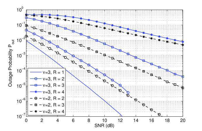
Figure 2: Outage probability for MMSE SC-FDE block transmission in a channels with memory lengths $\nu=2,3$, block length $L=10$ and different data rates $R=1,2,3,4$.

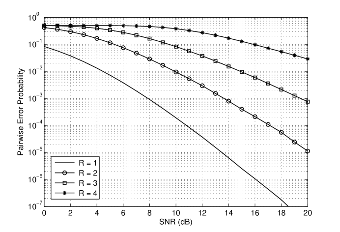
Figure 3: Achievable diversity order in MMSE SC-FDE block transmission in channels with memory length $\nu=3$, block length $L=10$ and different data rates $R=1,2,3,4$.

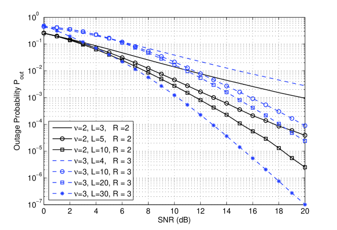
Figure 4: The effect of transmission block length on the diversity order for the settings $(\nu,R)=(2,2)$ and $(\nu,R)=(3,3)$.

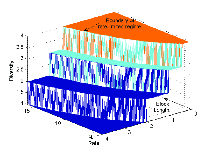
Figure 5: The tradeoff between diversity, rate, and block length for MMSE SC-FDE.

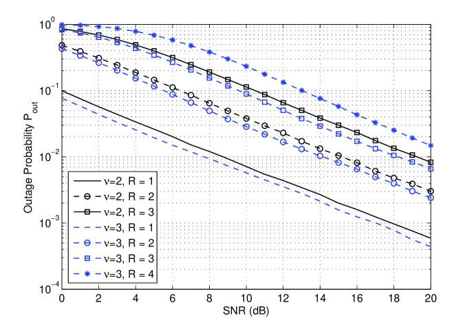
Figure 6: Average error probability for ZF SC-FDE block transmission for channel memory lengths $\nu=2,3$, block length $L=10$, and data rates $R=1,2,3,4$.

6 Discussion and Conclusion

In this paper we analyze the diversity of single-carrier cyclic-prefix block transmission with frequency-domain linear equalization. We show that MMSE SC-FDE may not fully capture the inherent frequency diversity of the ISI channels, depending on the system settings. We show that for such receivers, there exist a tradeoff between achievable diversity order, data rate and transmission block length. At high rates and low block-lengths, only diversity 1 is achieved, but by increasing the transmission block length and/or decreasing data rate, diversity order can be increased up to a maximum level of $\nu+1$, where $\nu$ is the channel memory length. We characterize the dependence on these two parameters in our results. Specifically, it is demonstrated that for MMSE SC-FDE, the results admit an interpretation in terms of operating regimes. As long as $R\leq\log\frac{L}{\nu}$, full diversity is achieved regardless of the exact value of the rate. When $R>\log\frac{L}{\nu}$ we are in a rate-limited regime where the diversity is affected by rate. In this regime, to maintain a given diversity while increasing the rate, each additional bit of spectral efficiency must be offset by at most doubling the block length. Naturally the block length cannot exceed the coherence time of the channel, thus putting practical limits on the performance of the equalizer.

We also prove that for zero-forcing SC-FDE, the diversity order is always one, independently of channel memory, transmission block length, or data rate.

For clarity and ease of exposition, the rates $R$ in this paper do not include the fractional rate loss incurred by the cyclic prefix. Once the fractional rate loss is included, the overall throughput will be equal to $R^{\prime}=\frac{L}{L+\nu}R$ which can be easily factored into all results.

Finally we would like to remark that the shorter version of this paper [17], which provides the outage analysis for MMSE equalizers, differs with the current paper in the following directions. First, [17] only treats MMSE equalizers whereas in this paper we have treated both MMSE and ZF equalizers. Secondly and more importantly, the analysis in [17] characterizes only the outage probability and its asymptotic behavior which does not suffice to obtain the diversity gain and, as discussed in Section 3.2, requires further analysis to establish the connection between the outage probability and the pair-wise error probability. Finally, we have provided a new and more intuitive proof for lemmas 1 and 2, which have key roles in characterizing the outage probability.

Appendix A Proof of Lemma 2

We start by showing that for any integer multiplier of $L$ denoted by $\tilde{L}=TL$, where $T\in\mathbb{N}$, and for any real-valued $m\in(0,\nu+1)$ we have

$$P\bigg{[}\sum_{k=1}^{\tilde{L}}\frac{1}{1+{{\sf SNR}}|\tilde{\lambda}_{k}|^{2}}>m\bigg{]}{\overset{\text{\Large.}}{=}}P\bigg{[}\sum_{k=1}^{L}\frac{1}{1+{{\sf SNR}}|\lambda_{k}|^{2}}>m\bigg{]},$$ (51)

where we have defined

$$\tilde{\boldsymbol{g}}_{1\times\tilde{L}}\stackrel{{\scriptstyle\scriptscriptstyle\triangle}}{{=}}[h_{0},\dots,h_{\nu},\underset{\tilde{L}-\nu-1}{\underbrace{0,\dots,0}}]\quad\mbox{and}\quad\{\tilde{\lambda}_{i}\}_{1\times\tilde{L}}\stackrel{{\scriptstyle\scriptscriptstyle\triangle}}{{=}}{\rm DFT}(\tilde{\boldsymbol{g}}),$$

and therefore, $\tilde{g}_{1\times\tilde{L}}$ is a zero-padded version of $g_{1\times L}$. Note that zero padding and applying a larger DFT size ($\tilde{L}$) is equivalent to sampling the Fourier transform of the $L$ data points at $\tilde{L}$ points. Based on the given set of DFT points $\{\lambda_{k}\}$ we can characterize the Fourier transform of $\boldsymbol{g}$ denoted by $G(\omega)$ at any specific frequency $\omega$ via

$$G(\omega)=\frac{1}{L}\sum_{i=1}^{L}\lambda_{i}\frac{1-e^{-jL\omega}}{1-e^{-j(\omega-\frac{2\pi(i-1)}{L})}}.$$ (52)

Therefore the DFT points $\{\tilde{\lambda}_{k}\}$ can be found by sampling the Fourier Transform $G(\omega)$ at frequenies $\omega=2\pi\frac{k-1}{\tilde{L}}$ for $k=1,\dots,\tilde{L}$. Therefore, we can describe the DFT points $\{\tilde{\lambda}_{k}\}$ in terms of $\{\lambda_{k}\}$ as

$$\tilde{\lambda}_{k}=\sum_{i=1}^{L}\lambda_{i}\;\underset{\stackrel{{\scriptstyle\scriptscriptstyle\triangle}}{{=}}\;\gamma_{i}}{\underbrace{\frac{1}{L}\cdot\frac{1-e^{-j\frac{(k-1)2\pi L}{\tilde{L}}}}{1-e^{-j(\frac{2\pi(k-1)}{\tilde{L}}-\frac{2\pi(i-1)}{L})}}}},\quad\mbox{for}\;k=1,\dots,\tilde{L}.$$ (53)

Moreover, since $\tilde{L}=TL$ we have

$$\tilde{\lambda}_{T(k-1)+1}=\lambda_{k},\quad\mbox{for}\;k=1,\dots,L.$$ (54)

By defining $\alpha_{k}\stackrel{{\scriptstyle\scriptscriptstyle\triangle}}{{=}}-\frac{\log|\lambda_{k}|^{2}}{\log{{\sf SNR}}}$ and $\tilde{\alpha}_{k}\stackrel{{\scriptstyle\scriptscriptstyle\triangle}}{{=}}-\frac{\log|\tilde{\lambda}_{k}|^{2}}{\log{{\sf SNR}}}$, for $k=1,\dots,L$ from (54) we get

$$\tilde{\alpha}_{T(k-1)+1}=\alpha_{k},\quad\mbox{for}\;k=1,\dots,L.$$ (55)

Also, from (53) we get

$$|\tilde{\lambda}_{k}|^{2}=\sum_{i=1}^{L}|\gamma_{i}|^{2}|\lambda_{i}|^{2}+\sum_{i=1}^{L}\sum_{l=1}^{L}\gamma_{i}\gamma^{*}_{l}\lambda_{i}\lambda^{*}_{l},\quad\mbox{for}\;k=1,\dots,\tilde{L}.$$ (56)

Since for any specific $\tilde{L}$ the coefficients $\{\gamma_{k}\}$ are constant values, we get

$$\lim_{{{\sf SNR}}\rightarrow\infty}\frac{\log|\gamma_{i}|^{2}|\lambda_{i}|^{2}}{\log{{\sf SNR}}}=\lim_{{{\sf SNR}}\rightarrow\infty}\frac{\log|\gamma_{i}|^{2}+\log|\lambda_{i}|^{2}}{\log{{\sf SNR}}}=\lim_{{{\sf SNR}}\rightarrow\infty}\frac{\log|\lambda_{i}|^{2}}{\log{{\sf SNR}}}\quad\Rightarrow\quad|\gamma_{i}|^{2}|\lambda_{i}|^{2}{\overset{\text{\Large.}}{=}}|\lambda_{i}|^{2}.$$

Let us also define $A\stackrel{{\scriptstyle\scriptscriptstyle\triangle}}{{=}}\sum_{i=1}^{L}\sum_{l=1}^{L}\gamma_{i}\gamma^{*}_{l}\lambda_{i}\lambda^{*}_{l}$ and $\alpha_{A}\stackrel{{\scriptstyle\scriptscriptstyle\triangle}}{{=}}-\frac{\log|A|}{\log\rho}$ which provides that $|A|=\rho^{-\alpha_{A}}$. Therefore (56) can be rewritten as

$${{\sf SNR}}^{-\tilde{\alpha}_{k}}{\overset{\text{\Large.}}{=}}\sum_{i=1}^{L}{{\sf SNR}}^{-\alpha_{i}}+\frac{A}{|A|}{{\sf SNR}}^{-\alpha_{A}}{\overset{\text{\Large.}}{=}}{{\sf SNR}}^{-\min_{i}\alpha_{i}}+\frac{A}{|A|}{{\sf SNR}}^{-\alpha_{A}},\quad\mbox{for}\;k=1,\dots,\tilde{L}.$$ (57)

Note that if $A<0$ we should have $\alpha_{A}\leq\min_{i}\alpha_{i}$ as otherwise for large values of ${{\sf SNR}}$ the RHS of (57) will be negative while the LHS is positive. Therefore, for $A<0$ we have ${{\sf SNR}}^{-\min_{i}\alpha_{i}}+\frac{A}{|A|}{{\sf SNR}}^{-\alpha_{A}}{\overset{\text{\Large.}}{=}}{{\sf SNR}}^{-\min_{i}\alpha_{i}}$. On the other hand, for $A\geq 0$ we have ${{\sf SNR}}^{-\min_{i}\alpha_{i}}+{{\sf SNR}}^{-\alpha_{A}}\;{\overset{\text{\Large.}}{\geq}}\;{{\sf SNR}}^{-\min_{i}\alpha_{i}}$. Hence, in summary we always have

$${{\sf SNR}}^{-\tilde{\alpha}_{k}}{\overset{\text{\Large.}}{=}}{{\sf SNR}}^{-\min_{i}\alpha_{i}}+\frac{A}{|A|}{{\sf SNR}}^{-\alpha_{A}}\;{\overset{\text{\Large.}}{\geq}}\;{{\sf SNR}}^{-\min_{i}\alpha_{i}}\quad\Rightarrow\quad\tilde{\alpha}_{k}\leq\min_{i}\alpha_{i}.$$ (58)

Now by using (55) and (56) we group the indices of the DFT points into two disjoint sets denoted by ${\cal A}\stackrel{{\scriptstyle\scriptscriptstyle\triangle}}{{=}}\{T(i-1)+1\;|\;i=1,\dots,L\}$ and ${\cal B}\stackrel{{\scriptstyle\scriptscriptstyle\triangle}}{{=}}\{1,\dots,\tilde{L}\}\backslash\{T(i-1)+1\;|\;i=1,\dots,L\}$. Therefore, by taking into account (55) we get

$$P\bigg{[}\sum_{k=1}^{\tilde{L}} \frac{1}{1+{{\sf SNR}}|\tilde{\lambda}_{k}|^{2}}>m\bigg{]}=P\bigg{[}\sum_{k\in{\cal A}}\frac{1}{1+{{\sf SNR}}|\tilde{\lambda}_{k}|^{2}}+\sum_{k\in{\cal B}}\frac{1}{1+{{\sf SNR}}|\tilde{\lambda}_{k}|^{2}}>m\bigg{]}$$

$$\;\;{\overset{\text{\Large.}}{=}}P\bigg{[}\sum_{k=1}^{L}\frac{1}{1+{{\sf SNR}}^{1-\alpha_{k}}}+\sum_{k\in{\cal B}}\frac{1}{1+{{\sf SNR}}^{1-\tilde{\alpha}_{k}}}>m\bigg{]}$$

$$=P\bigg{[}\sum_{k=1}^{L}\frac{1}{1+{{\sf SNR}}^{1-\alpha_{k}}}+\sum_{k\in{\cal B}}\frac{1}{1+{{\sf SNR}}^{1-\tilde{\alpha}_{k}}}>m\;\Big{|}\;\min_{i}\alpha_{i}<1\bigg{]}P(\min_{i}\alpha_{i}<1)$$

$$+P\bigg{[}\sum_{k=1}^{L}\frac{1}{1+{{\sf SNR}}^{1-\alpha_{k}}}+\sum_{k\in{\cal B}}\frac{1}{1+{{\sf SNR}}^{1-\tilde{\alpha}_{k}}}>m\;\Big{|}\;\min_{i}\alpha_{i}>1\bigg{]}P(\min_{i}\alpha_{i}>1).$$ (59)

Next, we further simplify the summands in (A). By taking into account that $\tilde{\alpha}_{k}\leq\min_{i}\alpha_{i}$, conditioning on the event $\{\min_{i}\alpha_{i}<1\}$ provides that $\sum_{k\in{\cal B}}\frac{1}{1+{{\sf SNR}}^{1-\tilde{\alpha}_{k}}}=0$ and the first summand becomes

$$P\bigg{[}\sum_{k=1}^{L}\frac{1}{1+{{\sf SNR}}^{1-\alpha_{k}}}+\sum_{k\in{\cal B}}\frac{1}{1+{{\sf SNR}}^{1-\tilde{\alpha}_{k}}}>m \;\Big{|}\;\min_{i}\alpha_{i}<1\bigg{]}$$

$$=P\bigg{[}\sum_{k=1}^{L}\frac{1}{1+{{\sf SNR}}^{1-\alpha_{k}}}>m\;\Big{|}\;\min_{i}\alpha_{i}<1\bigg{]}.$$ (60)

On the other hand, conditioning on the event $\{\min_{i}\alpha_{i}>1\}$ provides that $\sum_{k=1}^{L}\frac{1}{1+{{\sf SNR}}^{1-\alpha_{k}}}=L$ and $\sum_{k=1}^{L}\frac{1}{1+{{\sf SNR}}^{1-\alpha_{k}}}+\sum_{k\in{\cal B}}\frac{1}{1+{{\sf SNR}}^{1-\min_{i}\alpha_{i}}}\geq L$. Therefore, since $L>m\in(0,\nu+1)$ the second summand becomes

$$P\bigg{[}\sum_{k=1}^{L}\frac{1}{1+{{\sf SNR}}^{1-\alpha_{k}}}+\sum_{k\in{\cal B}}\frac{1}{1+{{\sf SNR}}^{1-\tilde{\alpha}_{k}}}>m \;\Big{|}\;\min_{i}\alpha_{i}>1\bigg{]}$$

$$=P\bigg{[}\sum_{k=1}^{L}\frac{1}{1+{{\sf SNR}}^{1-\alpha_{k}}}>m\Big{|}\min_{i}\alpha_{i}>1\bigg{]}=1.$$ (61)

Combining (A)-(A) establishes that

$$P\bigg{[}\sum_{k=1}^{\tilde{L}}\frac{1}{1+{{\sf SNR}}|\tilde{\lambda}_{k}|^{2}}>m\bigg{]} =P\bigg{[}\sum_{k=1}^{L}\frac{1}{1+{{\sf SNR}}^{1-\alpha_{k}}}>m\;\Big{|}\;\min_{i}\alpha_{i}<1\bigg{]}P(\min_{i}\alpha_{i}<1)$$

$$+P\bigg{[}\sum_{k=1}^{L}\frac{1}{1+{{\sf SNR}}^{1-\alpha_{k}}}>m\;\Big{|}\;\min_{i}\alpha_{i}>1\bigg{]}P(\min_{i}\alpha_{i}>1)$$

$$=P\bigg{[}\sum_{k=1}^{L}\frac{1}{1+{{\sf SNR}}|\lambda_{k}|^{2}}>m\bigg{]}$$ (62)

Therefore, to this end we have established that if $L\big{|}\tilde{L}$ then for any real-valued $m\in(0,\nu+1)$ we have

$$P\bigg{[}\sum_{k=1}^{\tilde{L}}\frac{1}{1+{{\sf SNR}}|\tilde{\lambda}_{k}|^{2}}>m\bigg{]}{\overset{\text{\Large.}}{=}}P\bigg{[}\sum_{k=1}^{L}\frac{1}{1+{{\sf SNR}}|\lambda_{k}|^{2}}>m\bigg{]}.$$

Now, lets set $\tilde{L}=L\times L^{\prime}$. As $L\big{|}\tilde{L}$ we have

$$P\bigg{[}\sum_{k=1}^{\tilde{L}}\frac{1}{1+{{\sf SNR}}|\tilde{\lambda}_{k}|^{2}}>m\bigg{]}{\overset{\text{\Large.}}{=}}P\bigg{[}\sum_{k=1}^{L}\frac{1}{1+{{\sf SNR}}|\lambda_{k}|^{2}}>m\bigg{]},$$ (63)

and since $L^{\prime}\big{|}\tilde{L}$ we have

$$P\bigg{[}\sum_{k=1}^{\tilde{L}}\frac{1}{1+{{\sf SNR}}|\tilde{\lambda}_{k}|^{2}}>m\bigg{]}{\overset{\text{\Large.}}{=}}P\bigg{[}\sum_{k=1}^{L^{\prime}}\frac{1}{1+{{\sf SNR}}|\lambda^{\prime}_{k}|^{2}}>m\bigg{]}.$$ (64)

(63) and (64) together establish the desired result.

References

• [1] H. Sari, G. Karam, and I. Jeanclaude, “Transmission techniques for digital terrestrial TV broadcasting,” IEEE Commun. Mag., vol. 33, pp. 100–109, February 1995.
• [2] D. Falconer, S. L. Ariyavisitakul, A. Benyamin-Seeyar, and B. Eidson, “Frequency domain equalization for single-carrier broadband wireless systems,” IEEE Commun. Mag., vol. 40, no. 4, pp. 58–66, April 2002.
• [3] M. V. Clark, “Adaptive frequency-domain equalization and diversity combining for broadband wireless communications,” IEEE J. Sel. Areas Commun., vol. 16, p. 1385 1395, October 1998.
• [4] N. Al-Dhahir, “Single-carrier frequency-domain equalization single-carrier frequency-domain equalization frequency-selective fading channels,” IEEE Commun. Lett., vol. 7, no. 7, 2001.
• [5] L. Zheng and D. Tse, “Diversity and multiplexing: a fundamental tradeoff in multiple-antenna channels,” IEEE Trans. Inf. Theory, vol. 49, no. 5, pp. 1073–1096, May 2003.
• [6] Z. Wang and F. Giannakis, “Complex field coding for OFDM over fading wireless channels,” IEEE Trans. Inf. Theory, vol. 49, no. 3, pp. 707–720, March 2003.
• [7] A. Ruiz, J. M. Cioffi, and S. Kasturia, “Discrete multiple tone modulation with coset coding for the spectrally shaped channel,” IEEE Trans. Commun., vol. 40, pp. 1012–1029, June 1992.
• [8] H. R. Sadjadpour, “Application of turbo codes for discrete multi-tone modulation schemes,” in Proc. Int. Conf. Comunications, vol. 2, Vancouver, BC, Canada, November 1999, pp. 1022– 1027.
• [9] J. Boutros and E. Viterbo, “Signal space diversity: a power- and bandwidth-efficient diversity technique for the Rayleigh fading channel,” IEEE Trans. Inf. Theory, vol. 44, no. 4, pp. 1453–1467, July 1998.
• [10] C. Tepedelenlioglu, “Maximum multipath diversity with linear equalization in precoded OFDM systems,” IEEE Trans. Inf. Theory, vol. 50, no. 1, pp. 232–235, January 2004.
• [11] C. Tepedelenlioglu and Q. Ma, “On the performance of linear equalizers for block transmission systems,” in Proc. IEEE Global Telecommunicaions Conference (Globecom), vol. 6, St. Louis, MO, November 2005.
• [12] A. Hedayat, A. Nosratinia, and N. Al-Dhahir, “Outage probability and diversity order of linear equalizers in frequency-selective fading channels,” in Proc. 38th Asilomar Conf. on Signals, Systems and Computers, vol. 2, Pacific Grove, CA, November 2004, pp. 2032– 2036.
• [13] D. T. M. Slock, “Diversity and coding gain of linear and deceision-feedback equalizers for frequency-selective SIMO channels,” in Proc. IEEE International Symposium of Information Theory (ISIT), Seattle, WA, July 2006, pp. 605–609.
• [14] W. Zhang, X. Ma, and A. Swami, “Maximum diversity of MIMO-OFDM schemes with linear equalizers,” in Proc. 4th IEEE Workshop on Sensor Array and Multi-channel Processing (SAM), July 2006.
• [15] E. K. Onggosanusi, A. G. Dabak, T. Schmidl, and T. Muharemovic, “Capacity analysis of frequency-selective mimo channels with suboptimal detectors,” in Proc. International Conference on Acoustics, Speech, and Signal Processing, May 2002, pp. 2369–2372.
• [16] T. M. Cover and J. A. Thomas, Elements of Information Theory, 2nd ed.   Hoboken, NJ: John Wiley and Sons, 2006.
• [17] A. Tajer and A. Nosratinia, “Diversity order of MMSE single-carrier frequency domain linear equalization,” in Proc. IEEE Global Communications Conference (Globecom), Washington, D.C., November 2007, pp. 1524 – 1528.