The effect of decoherence on mixing time in continuous-time quantum walks on one-dimension regular networks

S. Salimi , R. Radgohar
Faculty of Science, Department of Physics, University of Kurdistan, Pasdaran Ave., Sanandaj, Iran

Abstract

In this paper, we study decoherence in continuous-time quantum walks (CTQWs) on one-dimension regular networks. For this purpose, we assume that every node is represented by a quantum dot continuously monitored by an individual point contact(Gurvitz’s model). This measuring process induces decoherence. We focus on small rates of decoherence and then obtain the mixing time bound of the CTQWs on one-dimension regular network which its distance parameter is $l\geq 2$. Our results show that the mixing time is inversely proportional to rate of decoherence which is in agreement with the mentioned results for cycles in [29, 37]. Also, the same result is provided in [38] for long-range interacting cycles. Moreover, we find that this quantity is independent of distance parameter $l(l\geq 2)$ and that the small values of decoherence make short the mixing time on these networks.

1 Introduction

Quantum walk(QW) as a generalization of random walk(RW) is attracting great attention in many research areas, ranging from solid-state physics [1] to quantum computing [2]. Experimental implementations for the quantum walks have been presented in [3, 4, 5]. In recent years, two types of the quantum walks exist in the literature: the continuous-time quantum walks(CTQWs) [6, 7, 8, 9, 10] and the discrete-time quantum walks(DTQWs)  [11, 12, 13, 14, 15, 16]. The relationship between the CTQWs and the DTQWs has been considered in [17, 18, 19]. The CTQWs have been studied on star graph [20, 21], on direct product of cayley graphs [22], on quotient graphs [23], on odd graphs [24], on trees [25] and on ultrametric spaces [26]. All of these articles have focused on the coherent CTQWs. The effect of decoherence in the CTQWs has been studied on hypercube [27, 28], on cycle [29], on line [30, 31], on $N$-cycle [32] and on long-range interaction cycles [38]. Here, we study the CTQWs on one-dimension$(1D)$ networks with diatance parameter $l\geq 2$ which can be constructed as follows [33]: we construct an one dimensional ring lattice of $N$ nodes, each node of which is connected to its 2$l$ nearest neighbors($l$ on either side). The structure of one-dimension regular network with $N=8$ and $l=3$ is illustrated in Fig. 1. One-dimension regular networks have broad applications in various coupled systems, for example, Josephson junction arrays [34], small-world networks [35] and synchronization [36]. In our paper, the network nodes are represented by identical tunnel-coupled quantum dots(QDs). The walks are performed by an electron initially placed in one of the dots. An individual ballistic one-dimension point-contact is placed near each dot as ”detector” which its resistance is very sensitive to the electrostatic field generated by electron occupying the measured quantum dot. Decoherence is induced by continuous monitoring of each network node with nearby point contact. We focus on small rates of decoherence, then calculate the probability distribution and the mixing time bound of the CTQWs on one-dimension regular network with distance parameter $l\geq 2$. Our analytical results show that small decoherence can make short the mixing time in the CTQWs. The same result was produced for cycles in [29] and for long-range interacting cycles in [38]. Moreover, we show that for small rates of decoherence, the mixing time is independent of distance parameter $l(l\geq 2)$.

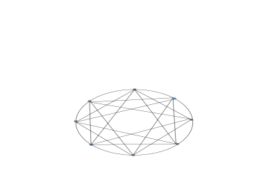
Figure 1: One-dimension regular network with $N=8$ and $l=3$

This paper is organized as follows:
In Sec. 2, we briefly review the properties of CTQWs on one-dimension regular networks. In Sec. 3, we study the decoherent CTQWs on the underlying network. We assume that the rate of decoherence is small and obtain the probability distribution, analytically in Sec. 4. The bound of the mixing time and its physical interpretation are provided in Sec. 5. Conclusions and discussions are given in the last part, Sec. 6.

2 CTQWs on $1D$ regular network

The properties of network is well characterized by the spectrum of adjacency matrix of associated graph. The network adjacency matrix($A$) is defined in the following way: $A_{ij}=1$ if nodes $i$ and $j$ are connected and otherwise $A_{ij}=0$. The Laplacian is defined as $L=A-D$, where $D$ is a diagonal matrix and $D_{j,j}$ is the degree of vertex $j$. Classically, the continuous-time random walks(CTRWs) are described by the master equation [1, 39]

$$\frac{d}{dt}p_{k,j}(t)=\sum_{l}T_{kl}p_{l,j}(t),$$ (1)

where $p_{k,j}(t)$ is the conditional probability to find the walker at time $t$ and node $k$ when starting at node $j$. The transfer matrix of the walk, $T$, is related to the adjacency matrix by $T=-\gamma L$. For the sake of simplicity, we assume that the transmission rate $\gamma$ of all bonds to be equal. The formal solution of Eq. (1) is

$$p_{k,j}(t)=\langle k|e^{Tt}|j\rangle.$$ (2)

The quantum-mechanical extension of the CTRW is called the continuous-time quantum walk(CTQW). The CTQW is obtained by replacing the Hamiltonian of system with the classical transfer operator, $H=-T$ [1, 39, 40].
The Hamiltonian matrix $H$ for one-dimension regular network is written as the following form [33]

$$H_{ij}=\langle i|H|j\rangle=\left\{\begin{array}[]{ll}-2\emph{m},&\hbox{if $i=j$;}\\ +1,&\hbox{if $i=j\pm z,z\in[1,\emph{l}]$;}\\ 0,&\hbox{Otherwise,}\end{array}\right.$$ (6)

that the basis vectors $|j\rangle$ associated with the nodes $j$ span the whole accessible Hilbert space. In these basis, the Schrödinger equation(SE) is

$$i\frac{d}{dt}|j\rangle=H|j\rangle,$$ (7)

where we set $m\equiv 1$ and $\hbar\equiv 1$. The Hamiltonian acting on the state $|j\rangle$ can be written as

$$H|j\rangle=-(2l+1)|j\rangle+\sum_{z=-l}^{l}|j+z\rangle,z\in Integers$$ (8)

which is the discrete version of the Hamiltonian for a free particle moving on a lattice. It is well known in solid state physics that the solutions of the SE for a particle moving freely in a regular potential are Bloch functions [41, 42]. Thus, the time independent SE is given by

$$H|\Phi_{n}\rangle=E_{n}|\Phi_{n}\rangle,$$ (9)

where eigenstates $|\Phi_{n}\rangle$ are Bloch states. The periodic boundary conditions require that $\Phi_{n}(N)=\Phi_{n}(0)$, where $\Phi_{n}(x)=\langle x|\Phi_{n}\rangle$. This restricts the $\theta$-values to $\theta=\frac{2\pi n}{N}$, where $n=0,1,\ldots,N-1$. The Bloch state $|\Phi_{n}\rangle$ can be expressed as a linear combination of the states $|j\rangle$ localized at nodes $j$,

$$|\Phi_{n}\rangle=\frac{1}{\sqrt{N}}\sum_{j=0}^{N-1}e^{-i\theta_{n}j}|j\rangle.$$ (10)

Substituting Eqs. (5) and (7) into Eq. (6) , we obtain the eigenvalues of the system as

$$E_{n}=-2l+2\sum_{j=1}^{l}cos(j\theta_{n}).$$ (11)

The time evolution of state $|j\rangle$ starting at time $t_{0}$ is given by $U(t,t_{0})|j\rangle$, where $U(t,t_{0})=\exp(-iH(t-t_{0}))$ is the quantum mechanical time evolution operator. Hence, the transition amplitude $\alpha_{k,j}(t)$ from state $|j\rangle$ at time $0$ to state $|k\rangle$ at time $t$ is

$$\alpha_{k,j}(t)=\langle k|e^{-iHt}|j\rangle.$$ (12)

Applying $E_{n}$ and $|\Phi_{n}\rangle$ to represent the nth eigenvalue and eigenvector of $H$, the classical and quantum transition probabilities between two nodes can be written as

$$P_{k,j}(t)=\sum_{n}e^{-tE_{n}}\langle k|\Phi_{n}\rangle\langle\Phi_{n}|j\rangle,$$ (13)

$$\pi_{k,j}(t)=|\alpha_{k,j}(t)|^{2}=|\sum_{n}e^{-itE_{n}}\langle k|\Phi_{n}\rangle\langle\Phi_{n}|j\rangle|^{2}.$$ (14)

3 The Decoherent CTQWs on $1D$ regular network

In this section, we investigate decoherence induced by the point contact(PC) detector measuring the occupation of one of the quantum dots(QDs) in a double-dot system. The measurement process is shown schematically in Fig. 2. We assume all electrons to be spin-less fermions and the tunneling between the PCs and the QDs to be negligible, but we take into account Coulomb interaction between electrons in the QD and the PC. We start with writing the Hamiltonian for the entire system. The total Hamiltonian is

$$H=H_{s}+\sum_{j=0}^{N-1}(H_{pc,j}+H_{int,j}),$$ (15)

where $H_{s}$, $H_{pc,j}$ and $H_{int,j}$ would be identified next.
Note that in this paper, quantum walk is defined over an undirected graph with $N$ nodes that each node is labeled by an integer $n\in[0,N-1]$. Also, we assume that the quantum walker has no internal state (i.e. simple quantum walker), so that we can describe its dynamics by a Hamiltonian of form [43]:

$$\begin{array}[]{cc}H_{s}=&\displaystyle\sum_{ij}\Delta_{ij}(t)(\hat{c}^{{\dagger}}_{i}\hat{c}_{j}+\hat{c}_{i}\hat{c}^{{\dagger}}_{j})-\displaystyle\sum_{j}E_{j}(t)\hat{c}^{{\dagger}}_{j}\hat{c}_{j},\\ &\\ =&\displaystyle\sum_{ij}\Delta_{ij}(t)(|i\rangle\langle j|+|j\rangle\langle i|)+\displaystyle\sum_{j}E_{j}(t)|j\rangle\langle j|\end{array}$$ (19)

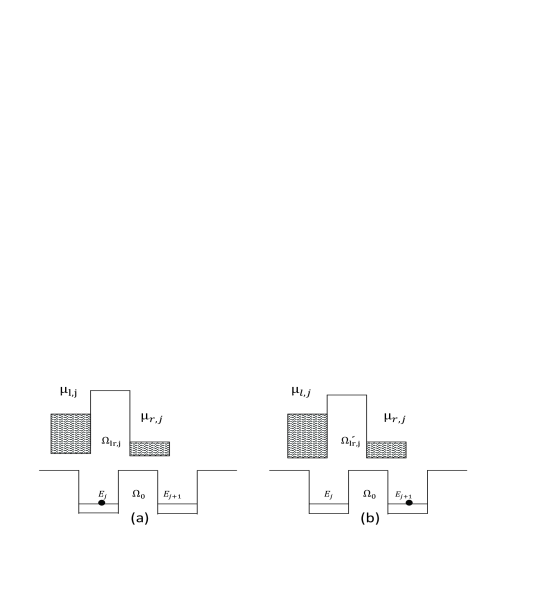
Figure 2: Fig. 2(a) shows point contact detector $j$ monitoring the electron in dot $j$ and Fig. 2(b) shows point contact detector $j$ when electron is placed in dot $j+1$. $\mu_{l,j}$ and $\mu_{r,j}$ are chemical potentials of left and right reservoirs of $j$th point contact, respectively. $E_{j}$ is the on-site node energy.

where $\hat{c}^{\dagger}_{j}(\hat{c}_{j})$ is creation (annihilation) operator and the walker at node $j$ corresponds to the quantum state $|j\rangle=\hat{c}_{j}^{{\dagger}}|0\rangle$. The first term in Eq. (13) is a ’hopping’ term with amplitude $\Delta_{ij}(t)$ along the edge ${ij}$ between nodes $i$ and $j$; the second term describes ’on-site’ node energies $E_{j}(t)$. We assume the hopping amplitude between connected sites to be constant and drop on-site energy terms (ie., ${E_{j}}=0,\forall j$). Also, for convenience, we renormalize the time so that it becomes dimensionless [44]. Thus, the simple quantum walker Hamiltonian has the form:

$$H_{s}=\frac{1}{4}\sum_{j=0}^{N-1}\sum_{z=1}^{l}(\hat{c}^{\dagger}_{j+z}\hat{c}_{j}+\hat{c}^{{\dagger}}_{j}c_{j+z}).$$ (20)

The tunneling Hamiltonian $H_{pc}$ describing this system can be written as

$$H_{pc,j}=\sum_{l}E_{l,j}\hat{a}^{\dagger}_{l,j}\hat{a}_{l,j}+\sum_{r}E_{r,j}\hat{a}^{\dagger}_{r,j}\hat{a}_{r,j}+\sum_{l,r}\Omega_{lr,j}(\hat{a}^{\dagger}_{l,j}\hat{a}_{r,j}+\hat{a}^{\dagger}_{r,j}\hat{a}_{l,j}),$$ (21)

where $\hat{a}^{\dagger}_{l,j}(\hat{a}_{l,j})$ and $\hat{a}^{\dagger}_{r,j}(\hat{a}_{r,j})$ are creation(annihilation) operators in the left and right reservoirs of point contact $j$, respectively. Also, $E_{l,j}$ and $E_{r,j}$ are the energy levels in the left and right reservoirs of detector, and $\Omega_{lr,j}$ is the hopping amplitude between the states $E_{l,j}$ and $E_{r,j}$. We assume that the hopping amplitude of $j$th point contact is $\Omega_{lr,j}$ when an electron occupies the left dot, and it is $\acute{\Omega_{lr,j}}$ when an electron occupies the right dot. Hence, we can represent the interaction term as

$$H_{int}=\sum_{l,r}\delta\Omega_{lr,j}\hat{c}_{j}^{\dagger}\hat{c}_{j}(\hat{a}_{l,j}^{\dagger}\hat{a}_{r,j}+\hat{a}^{\dagger}_{r,j}\hat{a}_{l,j}).$$ (22)

where ($\delta\Omega_{lr,j}=\Omega_{lr,j}-\acute{\Omega_{lr,j}}$). For simplicity, we assume that the hoping amplitudes are weakly dependent on states $E_{l,j}$ and $E_{r,j}$, so that $\Omega_{lr,j}=\Omega$, $\delta\Omega_{lr,j}=\delta\Omega$ and $\mu_{l,j}(\mu_{r,j})=\mu_{l}(\mu_{r})$. Gurvitz in [45] applied the Bloch-type equations for a description of the entire system with the large bias voltage($\mu_{l}-\mu_{r}$). He showed that the appearance of decoherence leads to the collapse of the density matrix into the statistical mixture in the course of the measurement processes. Using Eq. (5), this analysis for our model results in the following equation for the reduced density matrix

$$\begin{array}[]{cc}\frac{d}{dt}\rho_{j,k}(t)=&\frac{i}{4}[\displaystyle\sum_{z=-l}^{l}(\rho_{j,k+z}-\rho_{j+z,k})]-\Gamma(1-\delta_{j,k})\rho_{j,k}\\ &\\ =&\frac{i}{4}[\displaystyle\sum_{z=1}^{l}(\rho_{j,k+z}-\rho_{j+z,k}+\rho_{j,k-z}-\rho_{j-z,k})]-\Gamma(1-\delta_{j,k})\rho_{j,k}.\end{array}$$ (26)

4 Small Decoherence

In this section, we assume that the decoherence rate $\Gamma$ is small as ($\Gamma N\ll 1$) and consider its effect in the CTQWs on one-dimension regular network. For this end, we make use of the perturbation theory of linear operators ,as mentioned in [29], and rewrite Eq. (17) as the perturbed linear operator equation

$$\frac{d}{dt}\rho_{\alpha,\beta}(t)=\sum_{\mu,\nu=0}^{N-1}(iL_{(\alpha,\beta)}^{(\mu,\nu)}+U_{(\alpha,\beta)}^{(\mu,\nu)})\rho_{\mu,\nu}(t),$$ (27)

where $\alpha,\beta,\mu,\nu$ run from 0 to $N-1$. Also, $L_{(\alpha,\beta)}^{(\mu,\nu)}$ and $U_{(\alpha,\beta)}^{(\mu,\nu)}$ which are the row $(\mu,\nu)$ and column $(\alpha,\beta)$ elements of $N^{2}\times N^{2}$ matrices of $L$ and $U$ respectively, are defined as

$$L_{(\alpha,\beta)}^{(\mu,\nu)}=\frac{1}{4}[\sum_{z=-l}^{l}(\delta_{\alpha,\mu}\delta_{\beta,\nu-z}-\delta_{\alpha,\mu-z}\delta_{\beta,\nu})],$$ (28)

$$U_{(\alpha,\beta)}^{(\mu,\nu)}=-\Gamma\delta_{\alpha,\mu}\delta_{\beta,\nu}(1-\delta_{\alpha,\beta}).$$ (29)

Also, for our case, the initial conditions are

$$\rho_{\alpha,\beta}(0)=\delta_{\alpha,0}\delta_{\beta,0}.$$ (30)

Now, we want to obtain the eigenvalues and the eigenvectors of $L+U$. For this aim, we study the perturbed eigenvalue equation [29]

$$(L+U)(V+\tilde{V})=(\lambda+\tilde{\lambda})(V+\tilde{V}),$$ (31)

that $V$ is the corresponding eigenvector with eigenvalue $\lambda$ i.e. $LV=\lambda V$. Applying first-order perturbation theory of quantum mechanics, one can get

$$\tilde{\lambda}=V^{{\dagger}}UV.$$ (32)

We assume that $\epsilon_{\lambda}$ is the eigenspace with eigenvalue $\lambda$ and some of eigenvectors of $L$ (i.e. $\{V_{k}:k\in I\}$) span it. For the uniform linear combination, we can obtain $\tilde{\lambda}$ as following

$$\tilde{\lambda}=\sum_{k\in I}V_{j}^{{\dagger}}UV_{k}.$$ (33)

The solution of Eq. (18) is obtained by dropping the terms $\tilde{V}_{j}$ [29]

$$\rho(t)=\sum_{\lambda}e^{t(i\lambda+\tilde{\lambda})}\sum_{j\in\epsilon_{\lambda}}c_{j}V_{j}.$$ (34)

For unperturbed linear operator $L$, we have

$$\sum_{\mu,\nu=0}^{N-1}L_{(\alpha,\beta)}^{(\mu,\nu)}V_{(\mu,\nu)}^{(m,n)}=\lambda_{(m,n)}V_{(\alpha,\beta)}^{(m,n)},$$ (35)

that $\lambda_{(m,n)}$ is

$$\lambda_{(m,n)}=\sum_{z=1}^{l}\sin(\frac{\pi z(n+m)}{N})\sin(\frac{\pi z(m-n)}{N})$$ (36)

and $V_{(\mu,\nu)}^{(m,n)}$ is

$$V_{(\mu,\nu)}^{(m,n)}=\frac{1}{N}\exp(\frac{2\pi i}{N}(m\mu+n\nu)).$$ (37)

Using Eq. (24), one can obtain

$$\begin{array}[]{cc}U_{(m,n),(m^{\prime},n^{\prime})}&=(V^{(m,n)})^{{\dagger}}UV^{(m^{\prime},n^{\prime})}\\ &\\ &=-\frac{\Gamma}{N^{2}}\displaystyle\sum_{(a,b)}(1-\delta_{a,b})\exp(\frac{2\pi i}{N}[(m^{\prime}-m)a+(n^{\prime}-n)b])\\ &\\ &=-\Gamma\delta_{m^{\prime},m}\delta_{n^{\prime},n}+\frac{\Gamma}{N}\delta_{[(m^{\prime}-m)+(n^{\prime}-n)](modN),0}\end{array}$$ (43)

In what follows, we first find the degenerate eigenvalues of Eq. (27) and then calculate the eigenvalue perturbation terms:

(a) Diagonal element($m=n$):
Since $U$ is diagonal over the corresponding eigenvectors, there is not such degeneracy in our case [29]. For these eigenvalues, the correction terms are given by Eq. (29): $\tilde{\lambda}_{(m,m)}=-\Gamma\frac{(N-1)}{N}$.

(b) Zero$(m+n\equiv 0(modN))$:
Since the corresponding eigenvectors can not display in the linear combination of the initial state $\rho(0)$, this degeneracy is irrelevant to our problem [29].

(c) Off-diagonal elements:
By Eq. (29), the off-diagonal elements are non-zero if
$m+n\equiv m^{\prime}+n^{\prime}(modN)$.
To find degenerate eigenvalues satisfying the relation(c), we make divide the problem into two separate states as follows:

The state $l=1$: This state is equal to a cycle network, for which Eq. (27) reduces to $\lambda_{(m,n)}=\sin(\frac{\pi(n+m)}{N})\sin(\frac{\pi(m-n)}{N})$. $\lambda_{(m,n)}=\lambda_{(m^{\prime},n^{\prime})}$ results in $\sin(\frac{\pi(m+n)}{N})=\pm\sin(\frac{\pi(m^{\prime}+n^{\prime})}{N})$ and $\sin(\frac{\pi(m-n)}{N})=\pm\sin(\frac{\pi(m^{\prime}-n^{\prime})}{N})$. Thus, we have

$$\left\{\begin{array}[]{ll}m=n^{\prime}+N/2,n=m^{\prime}+N/2,&\hbox{for $N/2\leq m\leq N-1,N/2\leq n\leq N-1$;}\\ m=n^{\prime}-N/2,n=m^{\prime}-N/2,&\hbox{for $0\leq m<N/2,0\leq n<N/2$;}\\ m=n^{\prime}+N/2,n=m^{\prime}-N/2,&\hbox{for $N/2\leq m\leq N-1,0\leq n<N/2$;}\\ m=n^{\prime}-N/2,n=m^{\prime}+N/2,&\hbox{for $0\leq m<N/2,N/2\leq n\leq N-1$.}\end{array}\right.$$ (48)

The correction terms to these eigenvalues are $\tilde{\lambda}_{(m,n)}=-\Gamma\frac{(N-2)}{N}$.

The state $l\geq 2$: In this case, the structure of cycle network can be destroyed by $2l$ additional bonds in the network.
$\lambda_{(m,n)}=\lambda_{(m^{\prime},n^{\prime})}$ implies to
$\displaystyle\sum_{z=1}^{l}\sin(\frac{\pi z(n+m)}{N})\sin(\frac{\pi z(m-n)}{N})=\displaystyle\sum_{z=1}^{l}\sin(\frac{\pi z(n^{\prime}+m^{\prime})}{N})\sin(\frac{\pi z(m^{\prime}-n^{\prime})}{N})$.

One can see that there is not any degeneracy for this state. Thus, correction terms to these eigenvalues are $\tilde{\lambda}_{m,n}=-\Gamma\frac{(N-1)}{N}$.

The mixing time bound for the state $l=1$ was provided in  [29, 37].
In the following, we focus on the state $l\geq 2$(one-dimension regular network under condition $l\geq 2$) and in the end, compare our results with [29, 37]’s results for cycle.
Based on the above analysis, Eq. (25) can be written as

$$\rho(t)=\sum_{(m,n)}\frac{1}{N}(\delta_{m+n,0}+\delta_{m+n,N})V^{(m,n)}$$ (49)

and from Eq. (21), we have

$$\rho(0)=\sum_{(m,n)}\frac{1}{N}V^{(m,n)}.$$ (50)

Thus, the full solution is

$$\begin{array}[]{cc}\rho_{\alpha,\beta}(t)&=\frac{\delta_{\alpha,\beta}}{N}+\frac{1}{N^{2}}\displaystyle\sum_{(m,n)}(1-\delta_{[m+n](modN),0})e^{t(i\lambda_{(m,n)}+\tilde{\lambda}_{(m,n)})}\\ &\\ &\times\exp[\frac{2\pi i}{N}(m\alpha+n\beta)].\end{array}$$ (54)

The probability distribution $P_{j}(t)$ of the quantum walk is specified by the diagonal elements of the reduced density matrix, i.e.

$$\begin{array}[]{cc}P_{j}(t)&=\frac{1}{N}+\frac{1}{N^{2}}\displaystyle\sum_{(m,n)}(1-\delta_{[m+n](modN),0})\times[e^{-\Gamma\frac{N-1}{N}t}]\\ &\\ &\times\exp{[it\displaystyle\sum_{z=1}^{l}\sin(\frac{\pi z(m+n)}{N})\sin(\frac{\pi z(m-n)}{N})]}\times\exp[\frac{2\pi i}{N}(m+n)j].\end{array}$$ (58)

5 Mixing time

There are two distinct notions of mixing time for quantum walks in the literature:
Instantaneous mixing time: Instantaneous mixing time is defined as the first time instant at which the probability distribution of the walker’s position is $\epsilon$-close to the uniform distribution [46]. Thus, the instantaneous mixing time is

$$M_{inst,\epsilon}=min\{t:\|P_{j}(t)-\frac{1}{N}\|_{tv}<\epsilon\},$$ (59)

where here we use the total variation distance to measure the distance between two distributions $P,Q$: $\|P-Q\|_{tv}=\sum_{i}|P(i)-Q(i)|$.
Now by Eq. (34), we calculate an upper bound on the $M_{inst,\epsilon}$

$$\begin{array}[]{cc}|P_{j}(t)-\frac{1}{N}|&=e^{-\Gamma\frac{N-1}{N}t}|\frac{1}{N^{2}}\displaystyle\sum_{(m,n)}(\exp[{it\displaystyle\sum_{z=1}^{l}\sin(\frac{\pi z(m+n)}{N})\sin(\frac{\pi z(m-n)}{N})}]\\ &\\ &\times\exp[\frac{2\pi i}{N}(m+n)j])-\frac{1}{N}|.\end{array}$$ (63)

By noting that
$\exp[it\displaystyle\sum_{z=1}^{l}\sin(\frac{\pi z(m+n)}{N})\sin(\frac{\pi z(m-n)}{N})]\times\exp[\frac{2\pi i}{N}(m+n)j]\leq 1$,

one can obtain

$$|P_{j}(t)-\frac{1}{N}|\leq e^{-\Gamma\frac{N-1}{N}t}.$$ (64)

Thus, we have

$$\sum_{j=0}^{N-1}|P_{j}(t)-\frac{1}{N}|\leq Ne^{-\Gamma\frac{N-1}{N}t}.$$ (65)

Based on the above definition, the upper bound of instantaneous mixing time can be obtained in the following way:

$$Ne^{-\Gamma\frac{N-1}{N}t}\leq\epsilon,$$ (66)

and therefore,

$$M_{inst,\epsilon}\leq\frac{1}{\Gamma}\ln(\frac{N}{\epsilon})[1+\frac{1}{N-1}].$$ (67)

The $M_{inst,\epsilon}$ for cycles was provided in [29], that is

$$M_{inst,\epsilon}\leq\frac{1}{\Gamma}\ln(\frac{N}{\epsilon})[1+\frac{2}{N-2}].$$ (68)

These relations show that the instantaneous mixing time for one-dimension regular network with distance parameter $l(l\geq 2)$ is shorter than the one for cycle network. Also, this quantity is independent of distance parameter $l$ .

Average mixing time: To define the notion of average mixing time of CTQWs, we use the time-averaged probability distribution, i.e. $\bar{P}_{j}(t)=\frac{1}{\tau}\int_{0}^{\tau}P_{j}(t)dt$. The average mixing time measures the number of time steps required for the time-averaged probability distribution to be $\epsilon$-close to the limiting distribution [47], i.e.

$$M_{ave,\epsilon}=min\{t|\forall\tau>T:\|\bar{P}_{j}(t)-\frac{1}{N}\|_{tv}<\epsilon\}.$$ (69)

In the following, we want to obtain the lower bound of average mixing time for one-dimension regular network$(l\geq 2)$.
Applying Eq. (36) for large $N\gg 1$, we have

$$\|\bar{P}_{j}(t)-\frac{1}{N}\|\leq|\frac{1}{T}\int_{0}^{T}(e^{-\Gamma t}+\frac{1}{N})dt-\frac{1}{N}|=\frac{1}{\Gamma T}[1-e^{-\Gamma T}].$$ (70)

Summing over $j$ to calculate the total variation distance, we have

$$\frac{N}{\Gamma T}(1-e^{-\Gamma T})\leq\epsilon.$$ (71)

Then we assume that $\Gamma T\gg 1$ (since $N\gg 1$ and $\Gamma N\ll 1$, thus $T\gg N$) and achieve

$$M_{ave,\epsilon}\geq\frac{N}{\Gamma\epsilon},$$ (72)

which is similar to the average mixing time bound produced for cycle in [37].

Physical interpretation:
As mentioned in Sec. 3, we assumed the hopping amplitude between all of connected sites to be equal. Also, we supposed that every point-contact detector which is coupled to states localized on the corresponding node, measures the position of the particle in space of graph. Since these detectors identify the path of the walker took, quantum interference which is the result of an uncertainty in the path, is then lost and therefore the mixing time is independent of distance parameter $l$ [48]. However, one notes that this explanation might not be broadly accepted.

6 Conclusion

We studied the effect of small decoherence on one-dimension ring lattice of $N$ nodes in which every node is linked to its $2l$ nearest neighbors ($l\geq 2$ on either side). In our investigation, this network was represented by the system of identical tunnel-coupled quantum dots. As the detector, we used the point contact in close proximity to one of the dots. For description of the entire system, we applied the Bloch-type equations. Then, we calculated the probability distribution and the mixing time bound. We showed that the mixing time bound is independent of parameter $l(l\geq 2)$. Also, we observed that this quantity is inversely proportional to rate of decoherence, as mentioned in [29, 37]. Hence, decoherence can make short the mixing time on these networks. Moreover, we found that the instantaneous mixing time for one-dimension regular network is smaller than the one for cycle network.

References

• [1] G. H. Weiss, Aspect and Applications of the Random Walk, North-Holland, Amsterdam (1994).
• [2] M.A. Nielsen and I.L. Chuang. Quantum Computation and Quantum Information, Cambridge University Press, Cambridge, UK (2000).
• [3] C. A. Ryan, M. Laforest, J. C. Boileau and R. Laflamme, Phys. Rev. A 72, 062317 (2005).
• [4] B. C. Sanders et al., Phys. Rev. A 67, 042305 (2003).
• [5] P. Zhang, et al., Phys. Rev. A 75, 052310 (2007).
• [6] E. Agliari, O. MΓΌlken and A. Blumen, quant-ph/0903.3288 (2009).
• [7] A. J. Bessen, quant-ph/0609128 (2006).
• [8] M. A. Jafarizadeh, S. Salimi and R. Sufiani, Eur. Phys. J. B, 59, Pages: 199-216 (2007).
• [9] N. Konno, Physical Review E, Vol. 72, 026113 (2005).
• [10] M. A. Jafarizadeh and S. Salimi, J. Phys. A: Math. Gen., 39, Pages: 13295-13323 (2006).
• [11] K. Chisaki, M. hamada, N. Konno and E. Segawa, quant-ph/0903.4508 (2009).
• [12] M. Hamada, N. Konno and W. Mlotkowski, quant-ph/0903.4047 (2009).
• [13] C. M. Chandrashekar, R. Srikanth and R. Laflamme, Phys. Rev. A 77, 032326 (2008).
• [14] N. Konno, Quantum Information Processing, 1, Pages: 345-354 (2002).
• [15] M. A. Jafarizadeh and S. Salimi, Annals of Physics, 322, 1005-1033 (2007).
• [16] E. Feldman and M. Hillery, Phys. Lett A 324, 227 (2004).
• [17] A. Childs, quant-ph/0810.0312 (2009).
• [18] D. Alessandro, quant-ph/0902.3496 (2009).
• [19] A. Kempf and R. Portugal, quant-ph/0901.4237 (2009).
• [20] S. Salimi, Annals of Physics 324, Pages: 1185-1193 (2009).
• [21] X-P. Xu, J. Phys. A: Math. Theor. 42, 115205 (2009).
• [22] S. Salimi and M. Jafarizadeh, Commun. Theor. Phys. 51, Pages: 1003-1009 (2009).
• [23] S. Salimi, Int. J. Quantum Inf. 6, 945 (2008).
• [24] S. Salimi, Int. J. Theor. Phys. 47, Pages: 3298-3309 (2008).
• [25] N. Konno, Infinite Dimensional Analysis, Quantum Probability and Related Topics, Vol. 9, No. 2, Pages: 287-297 (2006).
• [26] N. Konno, International Journal of Quantum Information, Vol. 4, No. 6, Pages: 1023-1035 (2006).
• [27] F. W. Strauch, quant-ph/0808.3403 (2008).
• [28] G. Alagic and A. Russell, Phys. Rev A 72, 062304 (2005).
• [29] L. Fedichkin, D. Solenov and C. Tamon, Quantum Information and Computation, Vol 6, No. 3, Pages: 263-276 (2006).
• [30] A. Romanelli, R. Siri, G. Abal, A. Auyuanet and R. Donangelo, Phys. A, Vol. 347C. Pages: 137-152 (2005).
• [31] V. Kendon, B. Tregenna, in Proceedings of the 6th International Conference on Quantum Communication, Measurement and Computing, edu. J. H. Shapiro and O. Hirota (Rinton Press, Princeton, NJ, 2003), quant-ph/0210047.
• [32] V. Kendon, B. Tregenna, quant-ph/0301182 (2003).
• [33] X. Xu, F. Liu, Phys. Rev. E 77, 061127 (2008).
• [34] K. Wiesenfeld, Physica B 222, 315 (1996).
• [35] O. MΓΌlken, V. Pernice and A. Blumen, Phys. Rev. E 76, 051125 (2007).
• [36] I. V. Belykh, V. N. Belykh and M. Hasler, Physica D 195, 159 (2004).
• [37] V. Kendon, Math. Struct. in Comp. Sci. 17(6), Pages: 1169-1220 (2006).
• [38] S. Salimi and R. Radgohar, J. Phys. A: Math. Theor. 42, 475302 (2009).
• [39] N. Kampen, Stochastic Processes inPhysics and Chemistry(North-Holland, Amsterdam, 1990).
• [40] E. Farhi and S. Gutmann, Phys. Rev. A 58, 915 (1998).
• [41] O. M ulken and A. Blumen, Phys. Rev. E 71, 036128 (2005).
• [42] J. M. Ziman, Principles of the Theory of Solids (Cambridge University Press, Cambridge, England, 1972).
• [43] A. P. Hines and P. C. E. Stamp, quant-ph/0701088 (2007).
• [44] D. Solenov and L. Fedichkin, Phys. Rev. A 73, 012313 (2006).
• [45] A.Gurvitz, Phy. Rev B 56 (1997), 15215.
• [46] M. DrezgiΔ‡, A. P. Hines, M. Sarovar and S. Sastry, Quantum Information and Comp., vol. 9, 856 (2009).
• [47] D. Aharonov, A. Ambainis, J. Kempe and U. Vazirani, Proceedings of ACM Symposium on Theory of Computation (STOC’01), Pages: 50-59, (2001).
• [48] N. V. Prokof’ev and P. Stamp, Phys. Rev. A 74, 020102(R) (2006).