Isospin mixing and the continuum coupling in weakly bound nuclei

Abstract

The isospin breaking effects due to the Coulomb interaction in weakly-bound nuclei are studied using the Gamow Shell Model, a complex-energy configuration interaction approach which simultaneously takes into account many-body correlations between valence nucleons and continuum effects. We investigate the near-threshold behavior of one-nucleon spectroscopic factors and the structure of wave functions along an isomultiplet. Illustrative calculations are carried out for the $T$=1 isobaric triplet. By using a shell-model Hamiltonian consisting of an isoscalar nuclear interaction and the Coulomb term, we demonstrate that for weakly bound or unbound systems the structure of isobaric analog states varies within the isotriplet and impacts the energy dependence of spectroscopic factors. We discuss the partial dynamical isospin symmetry present in isospin-stretched systems, in spite of the Coulomb interaction that gives rise to large mirror symmetry breaking effects.

I Introduction

The charge independence of nuclear force gives rise to isospin symmetry [Hei32] ; [Wig37] and the formalism of isotopic spin has proven to be a very powerful concept in nuclear physics Wil69 . While useful, isospin symmetry is not perfectly conserved. On the hadronic level, isospin is weakly violated due to the difference in the masses of the up and down quarks Mil06 ; Mei08 ; Mac01 . The main source of isospin breaking in atomic nuclei lies, however, in the electromagnetic interaction [Ber72] .

The members of a nuclear isomultiplet, in particular mirror nuclei, provide a unique playground for studying isospin physics. The invariance under rotations in isospin space implies that energies of excited states in an isomultiplet should be identical; the deviations are usually attributed to the Coulomb force Wil69 ; Nol69 ; Len06 ; War06 ; Ben07 . However, for nuclear states close to, or above the reaction thresholds, the isospin breaking can be modified by the coupling to the particle continuum. Here, a spectacular example is the Thomas-Ehrman (TE) effect Ehr51 ; Tho52 ; Lan58 that occurs when one of the mirror states is unstable against particle emission due to a large asymmetry between proton and neutron emission thresholds. The resulting TE energy shifts strongly depend on the angular momentum content of the nuclear state and can be fairly large for low partial waves Com88 ; Wap02 .

The TE effect has also a direct consequence for the structure of mirror wave functions Aue00 ; Gri02 ; Tim08 ; Tim08a . Indeed, for near-threshold states, the configuration mixing involving scattering states strongly depends on (i) positions of particle emission thresholds in mirror systems (the binding energy effect) Oko08 , and (ii) different asymptotic behavior of neutron and proton wave functions. The latter leads to the universal behavior of cross sections Wigner ; Breit and spectroscopic factors (SFs) Mic07 ; Mic07a in the vicinity of a reaction threshold.

Recently, SFs and asymptotic normalization coefficients have been discussed in mirror systems within cluster approaches Tim08 ; Tim08a , and strong mirror symmetry-breaking in mirror SFs has been predicted. The main focus of this work is on the isospin mixing and mirror symmetry breaking in the isobaric analog states (IAS) of light nuclei. We show how the different asymptotic behavior within an isomultiplet and the isospin-nonconserving (INC) Coulomb interaction impact wave functions of IASs and resulting SFs. Our theoretical framework is the complex-energy continuum shell model, the Gamow Shell Model (GSM) Mic02 ; Bet02 ; Mic04 ; Mic09 . GSM is a configuration-interaction approach with a single-particle (s.p.) basis given by the Berggren ensemble Berggren1 which consists of Gamow (bound and resonance) states and the non-resonant scattering continuum.

This paper is organized as follows. Section II presents the details of the GSM calculations, with a particular focus on the treatment of the Coulomb potential and the recoil term. SFs in IASs are discussed in Sec. III. Therein, we study the dependence of SFs on the position of one- and two-particle thresholds. Our calculations are performed for prototypical $T=1$ isotriplet consisting of $J^{\pi}=0^{+}$ and 2⁺ IASs in ‘⁶He’, ⁶Li, and ‘⁶Be’. To remove the binding energy effect, we assume identical 1n/1p emission thresholds. In this way, we isolate the effect of the continuum coupling on isospin mixing, and study it in the vicinity of proton and neutron drip lines. The results for ⁶He, ⁶Li, and ⁶Be are discussed in Sec. IV by considering experimental and predicted one-particle thresholds. We point out that the conservation of isospin in the low-lying states of ⁶Be can be explained in terms of partial dynamical isospin symmetry present in the GSM wave functions of this isospin-aligned system. Finally, the conclusions are contained in Sec. V.

II The model

The GSM Hamiltonian is diagonalized in the many-body Slater determinants spanned upon the Berggren s.p. basis. The many-body resonant states of GSM obey the generalized variational principle Rot09 ; they are obtained using the generalized Davidson procedure that has been developed analogously to the generalized Lanczos procedure in the context of GSM (see Refs. Mic02 ; Mic09 for details).

We assume in the following that the nucleus can be described as a system of $n_{\pi}$ valence protons or $n_{\nu}$ valence neutrons evolving around a closed core. Since our discussion concerns the isobaric triplet ⁶He-⁶Li-⁶Be, we take ⁴He as a core. Consequently, the nuclei ⁵He and ⁵Li can be considered as one-particle systems, and ⁶He, ⁶Li, and ⁶Be as two-particle systems. In calculations involving ⁵He and ⁶He, the s.p. basis is generated by a Woods-Saxon (WS) potential with the radius $R_{0}$=2 fm, diffuseness $d$=0.65 fm, and spin-orbit strength $V_{\rm so}$=7.5 MeV. The depth of the central potential $V_{0}$ has been varied to move the binding energy of a one-neutron system, ⁵He (i.e., the one-neutron threshold). For $V_{0}$=47 MeV (the “⁵He” parameter set), this potential reproduces energies and widths of experimental $3/2_{1}^{-}$ and $1/2_{1}^{-}$ resonances in ⁵He.

The GSM results should be free from spurious center-of-mass (CM) motion. To cope with this problem in our GSM approach, we adopt a system of intrinsic nucleon-core coordinates inspired by the Cluster Orbital Shell Model (COSM) Suz88 ; Suz90 . In the COSM coordinates, the translationally-invariant GSM Hamiltonian can be written as:

$$\textit{H}=\sum_{i=1}^{n_{\pi}+n_{\nu}}\left[\frac{\bm{p}_{i}^{2}}{2\mu}+U_{i}\right]+\sum_{i<j}^{n_{\pi}+n_{\nu}}\left[V_{ij}+\frac{1}{A_{c}}\bm{p}_{i}\bm{p}_{j}\right],$$ (1)

where $\mu$ is the reduced mass of the nucleon+core system, $U_{i}$ is the one-body WS potential representing the field of the core, $V_{ij}$ is the two-body residual interaction between valence nucleons, and the two-body term $A_{c}^{-1}\bm{p}_{i}\bm{p}_{j}$, with $A_{c}$ being the mass of the core, takes into account the recoil of the active nucleons.

The modified finite-range surface Gaussian interaction (MSGI) used in this study is a variant of the finite-range surface Gaussian interaction (SGI) Mic04 . In order to discuss the motivation behind MSGI, we begin with the definition of the two-body residual interaction SGI:

$$V_{J,T}^{SGI}(\bm{r_{1}},\bm{r_{2}})$$ (2)

$$= V_{0}(J,T)\exp\left[-\left(\frac{\bm{r_{1}}-\bm{r_{2}}}{\mu_{I}}\right)^{2}\right]\delta(r_{1}+r_{2}-2R_{0})$$

$$= V_{0}(J,T)\sum_{\ell=0}^{+\infty}\exp\left(-\frac{r_{1}^{2}+r_{2}^{2}}{\mu_{I}^{2}}\right)\delta(r_{1}+r_{2}-2R_{0})$$

$$\times i^{\ell}(2\ell+1)~{}j_{\ell}\left(\frac{2r_{1}r_{2}}{i\mu_{I}^{2}}\right)\bm{Y}_{\ell}(\hat{r}_{1})\cdot\bm{Y}_{\ell}(\hat{r}_{2}),$$

where $\mu_{I}$ is the interaction range; $V_{0}(J,T)$ is the strength of the interaction, which depends on the total angular momentum $J$ and isospin $T$; $R_{0}$ is the radius of the one-body Woods-Saxon potential; and $\hat{r}=\bm{r}/r$.

The contact term represented by the Dirac delta function in Eq. (2) generates unwanted divergences in momentum space analogous to those present for zero-range interactions. To rectify this problem, we replace the radial form factors of the multipole expansion of SGI by separable terms, chosen independently of $\ell$ for simplicity. With this choice, the modified interaction MSGI reads:

$$V_{J,T}^{MSGI}(\bm{r_{1}},\bm{r_{2}})$$ (3)

$$= V_{0}(J,T)\exp\left[-\left(\frac{r_{1}-R_{0}}{\mu_{I}}\right)^{2}\right]\exp\left[-\left(\frac{r_{2}-R_{0}}{\mu_{I}}\right)^{2}\right]$$

$$\times F(R_{0},r_{1})F(R_{0},r_{2})\sum_{\ell=0}^{\ell_{\rm max}}\bm{Y}_{\ell}(\hat{r}_{1})\cdot\bm{Y}_{\ell}(\hat{r}_{2}),$$

where $\displaystyle F(R_{0},r)=\left[1+\exp\left(\frac{r-2R_{0}-r_{F}}{\mu_{F}}\right)\right]^{-1}$ (with $r_{F}=1$ fm and $\mu_{F}=0.05$ fm) is a Fermi function which makes MSGI practically vanish at $r>2R_{0}$.

The surface character of MSGI is incorporated through the Gaussians centered at $R_{0}$. Due to the separability of the radial form factors and the presence of the radial Fermi cut-off, two-body radial matrix elements of MSGI are products of one-dimensional integrals which are non-zero only for $0<r<2R_{0}$; hence, they are as easy to calculate as the radial integrals of SGI Mic04 . The range of MSGI is fixed at $\mu_{I}=1$ fm. The coupling constants $V_{0}(J,T)$ are adjusted to the binding energies ground state (g.s.) and first 2⁺ state of ⁶He and ⁶Be. It is important to point out that the two-body nuclear GSM interaction of Eq. (3) is isoscalar by construction. That is, in our work, we do not address the question of INC nuclear forces.

The valence space for neutrons and protons consists of all partial waves of angular momentum $\ell=$ 0, 1, and 2. Consequently, the orbital angular momentum cut-off in Eq. (3) is $\ell_{\rm max}$=2. The $p_{3/2}$ wave functions include a $0p_{3/2}$ resonant state and $p_{3/2}$ non-resonant scattering states along a complex contour enclosing the $0p_{3/2}$ resonance in the complex $k$-plane. For the remaining partial waves, i.e., $s_{1/2}$, $p_{1/2}$, $d_{3/2}$, and $d_{5/2}$, we take the non-resonant contour along the real-$k$ axis (the broad $0p_{1/2}$ resonant state plays a negligible role in the g.s. wave function of ⁶He and ⁶Be). For all contours, the maximal momentum value is $k_{\rm max}=4$ fm^-1. The contours have been discretized with up to 80 points.

In calculations for systems having valence protons, one has to consider explicitly the Coulomb interaction. For ⁵Li, it is represented by a one-body Coulomb potential of ⁴He. In principle, one could approximate it by a Coulomb potential of a uniformly charged sphere of radius $R_{0}$. However, such a potential is inconvenient to use because of its non-analytic behavior at $R_{0}$. Therefore, we use the dilatation-analytic form of the Coulomb potential $U^{(Z)}_{c}$ Sai77 ; Myo98 ; idb08 , generated by a Gaussian proton density:

$$U^{(Z)}_{c}(r) = Ze^{2}~{}\frac{{\rm erf}(r/\nu_{c})}{r}.$$ (4)

In the above equation, $\nu_{c}=4R_{0}/(3\sqrt{\pi})$, where $R_{0}$ is the radius of the WS potential, and $Z$ is the number of protons of the target, e.g., $Z$=2 for the “proton + ⁴He core” system. The above choice of $R_{0}$ assures that the Coulomb potential given by Eq. (4) and the uniformly charged sphere potential are equal at $r$=0.

The nucleus ⁶Be has two valence protons outside the ⁴He core. Consequently, the two-body Coulomb interaction $V_{c}$ has to be considered. Unfortunately, the calculation of two-body matrix elements of $V_{c}$ in a basis generated by the one-body part of the GSM Hamiltonian is impractical because of difficulties associated with computing two-dimensional integrals with the complex scaling method for resonant and scattering basis states. A more practical procedure can be developed if one notices that at large distances the Coulomb term $U^{(2)}_{c}+V_{c}$ must behave as $\displaystyle U^{(3)}_{c}(r)\sim 3~{}e^{2}~{}r^{-1}$. Consequently, since $U^{(Z)}_{c}$ is additive in $Z$, one can rewrite the Coulomb interaction in the ⁶Be Hamiltonian as $U^{(3)}_{c}+(V_{c}-U^{(1)}_{c})$. The short-range character of the operator $V_{c}-U^{(1)}_{c}$ suggests using the method which consists of expanding two-body operators in a truncated basis of harmonic oscillator (HO) states Gaute_Morten :

$$V_{c}-U^{(1)}_{c} \simeq [V_{c}-U^{(1)}_{c}]^{(N)}$$ (5)

$$= P_{N}(V_{c}-U^{(1)}_{c})P_{N}$$

$$= \sum_{\alpha\beta\gamma\delta}^{N}|\alpha\beta\rangle\langle\alpha\beta|V_{c}-U^{(1)}_{c}|\gamma\delta\rangle\langle\gamma\delta|$$

where Greek letters label HO states, $N$ is the number of HO states used in a given partial wave, and $P_{N}$ is a projector:

$$P_{N}=\sum_{\alpha\beta}^{N}|\alpha\beta\rangle\langle\alpha\beta|.$$ (6)

To justify the approximation stated in Eq. (5), let us consider a normalizable two-body eigenstate $|\Psi\rangle$. $|\Psi\rangle$ can be either bound or resonant because resonant states become integrable when complex scaling is applied to radial coordinates Gya71 . In this case, $|\Psi\rangle$ can be expanded in the HO basis used in Eq. (5). According to Eq. (6), $P_{N}|\Psi\rangle\rightarrow|\Psi\rangle$ when $N\rightarrow+\infty$. Hence, the matrix elements of the operator $[V_{c}-U^{(1)}_{c}]^{(N)}$ involving two-body normalizable states converge to those of $V_{c}-U^{(1)}_{c}$ when $N\rightarrow+\infty$, i.e. $\displaystyle\langle\Psi_{f}|[V_{c}-U^{(1)}_{c}]^{(N)}|\Psi_{i}\rangle\rightarrow\langle\Psi_{f}|V_{c}-U^{(1)}_{c}|\Psi_{i}\rangle$. The latter equality is independent of the basis used to expand $|\Psi_{i}\rangle$ and $|\Psi_{f}\rangle$. In particular, one can use the Berggren basis for this purpose. The short-range character of the operator $V_{c}-U^{(1)}_{c}$ implies that $\displaystyle\langle\Psi_{f}|[V_{c}-U^{(1)}_{c}]^{(N)}|\Psi_{i}\rangle$ should converge rapidly with $N$. This argument can be easily generalized for many-body wave functions with more than two particles.

The matrix elements in Eq. (5) can be calculated efficiently using the Brody-Moshinsky transformation. The computation of one-body overlap integrals between Berggren basis and HO states is straightforward, as these always converge along the real axis due to the Gaussian tail of HO states; hence, no complex scaling is needed. The recoil term in Eq. (1) can be treated in the same way as the Coulomb interaction, i.e., by expanding $\bm{p}_{i}$ in a HO basis Gaute_Morten . The attained precision of calculations on energies and widths is better than 0.2 keV for calculations without recoil and Coulomb terms, and it is around 1 keV for the full GSM scheme.

It has to be noted that because our model involves a core, our treatment of the Coulomb interaction is not exact. In particular, we neglect the contribution to the exchange term arising from the core protons. We also ignore other known charge-symmetry breaking electromagnetic terms such as the Coulomb spin-orbit interaction.

III Spectroscopic factors in isobaric analog states

The SF in the GSM framework is given by the real part of the squared norm $S^{2}$ of the overlap integral between initial and final state in the reaction channel Mic07 ; Mic07a . The imaginary part of $S^{2}$, which is an uncertainty of ${\cal R}e$($S^{2}$), vanishes if both states in nuclei $A$ and $A$–1 are bound. Using a decomposition of the s.p. channel $(\ell,j)$ in the complete Berggren basis, one obtains:

$$S^{2}=\int\sum_{\mathcal{B}}\langle\widetilde{\Psi^{J_{A}}_{A}}||a^{+}_{\ell j}(\mathcal{B})||\Psi^{J_{A-1}}_{A-1}\rangle^{2}$$ (7)

where $a^{+}_{\ell j}(\mathcal{B})$ is a creation operator associated with a s.p. basis state $|u_{\mathcal{B}}\rangle$ and the tilde symbol above bra vectors signifies that the complex conjugation arising in the dual space affects only the angular part and leaves the radial part unchanged. Since Eq. (7) involves summation over all discrete Gamow states and integration over all scattering states along the complex contour, the final result is independent of the s.p. basis assumed. This feature is crucial for loosely bound states and near-threshold resonances, where the coupling to the non-resonant continuum can no longer be neglected. Indeed, the contribution of the scattering continuum to SFs can be as large as 25% in such cases Mic07 ; Mic07a .

In the context of this study, the direct use of Eq. (7) is impractical when assessing effects related to the configuration mixing. Indeed, because of the presence of reduced matrix elements, $S^{2}\neq 1$ in the absence of many-body correlations, and its value depends on $j$, $J_{A-1}$, and $J_{A}$. Hence, we choose to renormalize $S^{2}$ by dividing it by the extreme single-particle value (obtained by neglecting two-body interactions). Within this convention, $S^{2}=1$ if configuration mixing is absent.

The SFs for the two-neutron (⁶He) and two-proton (⁶Be) g.s. configurations considered in our work correspond to the $[{{}^{5}}{\rm He}({\rm g.s.})\otimes\nu p_{3/2}]^{0^{+}}$ and $[{{}^{5}}{\rm Li}({\rm g.s.})\otimes\pi p_{3/2}]^{0^{+}}$ channels, respectively. For the $T=1$ IASs in ⁶Li, we consider two channels: $[{{}^{5}}{\rm He}({\rm g.s.})\otimes\pi p_{3/2}]^{0^{+}}$ and $[{{}^{5}}{\rm Li}({\rm g.s.})\otimes\nu p_{3/2}]^{0^{+}}$.

III.1 Stability of HO expansion

The quality of the HO expansion of Eq. (5) has been numerically checked for both the Coulomb interaction and recoil term. Figure 1 displays the convergence with respect to the number of HO states used in the expansion for the total energy, width, and SF (real and imaginary part) of g.s. configurations in ⁶Be and ⁶He. For ⁶Be, the results obtained by assuming the inert core (no recoil, i.e., $A_{c}=+\infty$ in Eq. (1)) are also presented. It is seen that with nine HO states per partial wave, one obtains excellent convergence for both energies and wave functions, the latter being represented by SFs. For the complex energy, the associated numerical error is of the order of 2 keV, and this is well below other theoretical uncertainties of the model.

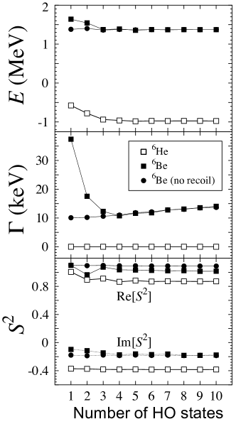
Figure 1: The numerical check of the HO expansion (5) for the total energy (top), width (middle), and spectroscopic factor (bottom) for g.s. configurations of ⁶Be (filled symbols) and ⁶He (open squares). The GSM predictions are plotted as a number of HO states used in the expansion. The HO length is $b$=2 fm Gaute_Morten .

III.2 Threshold dependence of spectroscopic factors

The GSM SFs for ⁶He and ⁶Be are shown in the left column of Fig. 2. The results are plotted as a function of one-nucleon separation energy ($S_{1n}$ for ⁶He and $S_{1p}$ for ⁶Be) for three different values of the one-particle threshold energy $E_{T}$ (i.e., negative of one-nucleon separation energy) in one-nucleon systems: ⁵He and ⁵Li.

For the bound $A$=5 systems ($E_{T}=-1.5$ MeV), the SFs in ⁶He and ⁶Be are different in the whole range of separation energies considered. The difference of the SFs reach the maximum at the one-nucleon emission threshold. As the separation energy increases (both nuclei become more particle-bound) both SFs slowly approach the value of one, as expected from simple shell-model considerations Mic07 . A characteristic irregularity in the $\ell=1$ neutron SF at the neutron emission threshold of ⁶He is the Wigner cusp. The cusp is absent in the mirror system ⁶Be as a result of the different asymptotic behavior of the proton wave function Wigner .

The energy dependence of SFs changes if the $A$=5 system happens to be at the particle emission threshold ($E_{T}$=0) or is unbound ($E_{T}$=0.5 MeV). In both situations, a significant difference of SFs in mirror states is seen in particle stable (positive $S_{1n}$ or $S_{1p}$) $A$=6 systems. One may also notice that the Wigner cusp disappears altogether if ⁵He becomes unbound (cf. $E_{T}$=0.5 MeV variant in Fig. 2).

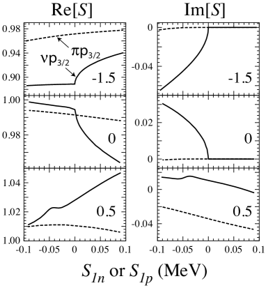
Figure 2: The spectroscopic factor $S=\sqrt{S^{2}}$, i.e., the real and imaginary parts of the square root of the overlap integral (7) corresponding to $\langle{{}^{6}}{\rm He}({\rm g.s.})|[{{}^{5}}{\rm He}({\rm g.s.})\otimes\nu p_{3/2}]^{0^{+}}\rangle$ (solid line) and $\langle{{}^{6}}{\rm Be}({\rm g.s.})|[{{}^{5}}{\rm Li}({\rm g.s.})\otimes\pi p_{3/2}]^{0^{+}}\rangle$ (dashed line) as a function of one-nucleon separation energy ($S_{1n}$ for ⁶He and $S_{1p}$ for ⁶Be) for three different values of one-particle threshold energy $E_{T}=-1.5$, 0, and 0.5 MeV in $A$=5 systems (indicated at the right of each panel).

It is interesting to notice that SFs can be greater than 1 if the state of the $A-1$ system is particle unstable. This unusual situation (see, e.g., ${\cal R}e$($S$) in ⁶He for $E_{T}=+0.5$ MeV) is discussed below.

The imaginary part of the expectation value of an operator in a resonant state can be interpreted as the uncertainty in the determination of this expectation value due to the possibility of decay during the measuring process Ber96 ; Civ99 ; Hat08 ; Hat09 . Figure 2 (right column) shows the uncertainty ${\cal I}m$($S$) of SFs displayed in Fig. 2 (left column). The uncertainty vanishes if the wave functions in both $A$=6 and $A$=5 systems are bound with respect to the particle emission. Note that in Fig. 2, the appearance of ${\cal R}e$($S$)$>1$ cannot be fully explained by the ${\cal I}m$($S$) plot. Indeed, for ⁶He at $E_{T}$=0.5 MeV and $0.05<S_{1n}<0.1$ MeV, ${\cal R}e$($S$)$>1$ corresponds to $|{\cal I}m$($S)|\simeq 0$.

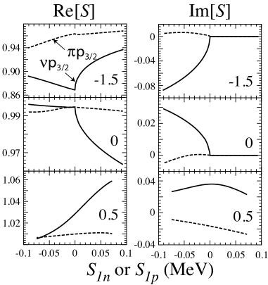
Figure 3: Same as in Fig. 2 except for $\langle{{}^{6}}{\rm Li}(T=1)|[{{}^{5}}{\rm Li}({\rm g.s.})\otimes\nu p_{3/2}]^{0^{+}}\rangle$ (solid line) and $\langle{{}^{6}}{\rm Li}(T=1)|[{{}^{5}}{\rm He}({\rm g.s.})\otimes\pi p_{3/2}]^{0^{+}}\rangle$ (dashed line) as a function of one-nucleon separation energy ($S_{1n}$ for the former and $S_{1p}$ for the latter) for three different values of one-particle threshold energy $E_{T}=-1.5$, 0, and 0.5 MeV in $A$=5 systems. The proton and neutron threshold energies are assumed to be identical.

For the $J^{\pi}=0^{+}$ IAS in ⁶Li, we consider two different SFs for the $(\ell,j)=p_{3/2}$ channel, associated with adding a proton to ⁵He or a neutron to ⁵Li (see Fig. 3). They are plotted in Fig. 3 as a function of one-proton (or one-neutron) separation energy. The channel wave functions $|[{{}^{5}}{\rm He}({\rm g.s.})\otimes\pi p_{3/2}]^{0^{+}}\rangle$ and $|[{{}^{5}}{\rm Li}({\rm g.s.})\otimes\nu p_{3/2}]^{0^{+}}\rangle$ are obviously not orthogonal, as they both share the dominant $|[{{}^{4}}{\rm He}({\rm g.s.})\otimes\pi~{}0p_{3/2}\otimes\nu~{}0p_{3/2}]^{0^{+}}\rangle$ component. The two considered SFs for ⁶Li differ only by continuum couplings induced in the proton and neutron channels. Comparing Fig. 2 and Fig. 3, one can see $p_{3/2}$ proton and neutron SFs factors are very similar in both cases. Still, slight differences are present. For instance, at $E_{T}=0.5$ MeV, small irregularities seen in ⁶He SFs are absent in the neutron SF for ⁶Li. A close inspection of proton SFs for ⁶Li reveals the presence of threshold cusps at zero separation, absent on the ⁶Be case. This effect can be explained in terms of the channel coupling, or flux conservation Mic07 ; Mic07a . Indeed, since in our model calculations both proton and neutron channels open at threshold energy, the coupling between proton and neutron channels can generate non-analyticities in proton SFs, even though Wigner estimates for proton cross sections are analytical at the threshold energy.

To study the sensitivity of results to the CM treatment, we carried out a set of calculations assuming the inert core (no recoil). The results are practically identical to those of Figs. 2 and 3. The only noticeable difference is the absence of a small fluctuation at $S_{1n}$$\approx$–0.05 MeV seen in the real and imaginary parts of SF for ⁶He.

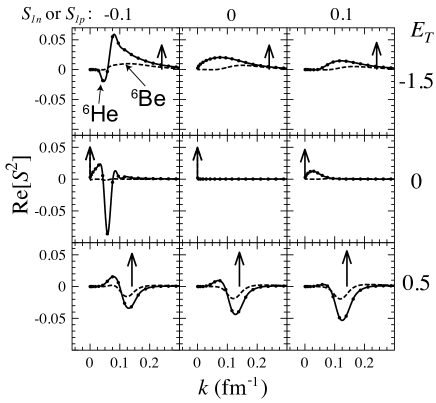
Figure 4: The distribution of the real part of ${\cal R}e$($S_{\rm c}^{2}$) in ⁶He (solid line) and ⁶Be (dashed line) with respect to the $3/2^{-}$ scattering states of the ⁵He and ⁵Li systems, ordered according to their real-$k$ value. The calculations were performed for three different values of one-particle threshold energy $E_{T}$=$-1.5$ MeV (top), 0 (middle), and 0.5 MeV (bottom) in $A$=5 systems. The arrows indicate contributions from resonant states. In order to facilitate presentation, the pole contributions were multiplied by a scaling factor of 0.05.

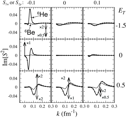
Figure 5: Same as in Fig. 4, except for the imaginary part of ${\cal I}m$($S_{\rm c}^{2}$). The arrows indicate contributions from $0p_{3/2}$ resonant states if those are not negligible. In order to facilitate presentation, the pole contributions were multiplied by the scaling factors indicated in the figure.

Another reason for the occurrence of ${\cal R}e$($S$)$>1$ in some cases, is the interplay between a final state $\Psi^{J_{A-1}}_{A-1}\equiv\Psi^{J_{A-1}}_{A-1;{\rm R}}$ (the many-body resonance) and states of the non-resonant scattering continuum $\{\Psi^{J_{A-1}}_{A-1;{\rm c}}\}$ with energies close to the resonance energy Ber96 . The contributions to SFs $S_{\rm c}$ in ⁶He and ⁶Be coming from the non-resonant continuum are shown in Figs. 4 and 5 together with contributions from resonant states.

In all situations, the contribution of the Gamow resonance to ${\cal R}e$($S^{2}$) is dominant. It is interesting to note that the impact of the non-resonant continuum does depend on $E_{T}$ and $S_{1p}/S_{1n}$. For $E_{T}\leq 0$ and $S_{1p}/S_{1n}\geq 0$, i.e., for $A$=5 and $A$=6 bound ground states, the non-resonant continuum contribution is basically negligible. This is also the case for ⁶Be when $E_{T}\leq 0$ and $S_{1p}/S_{1n}<0$, i.e., for a bound ⁵Li but an unbound ⁶Be. However, when either the $A$=5 g.s. is unbound ($E_{T}>0$) or $E_{T}\leq 0$ and $S_{1p}/S_{1n}<0$ for ⁶He, i.e., when ⁶He is unbound with respect to a bound ⁵He, the non-resonant continuum plays a significant role in both real and imaginary parts. In particular, when $E_{T}>0$ and $S_{1p}/S_{1n}\geq 0$, the contribution from the non-resonant continuum ${\cal R}e$($S_{\rm c}^{2}$) becomes negative, which translates into a value of ${\cal R}e$($S^{2}$) that exceeds one. One can also see that ${\cal I}m$($S_{\rm c}^{2}$) is comparable to ${\cal R}e$($S_{\rm c}^{2}$), even though this does not occur every time ${\cal R}e$($S^{2}$)$>1$. The lesson learned from this discussion is that the SF obtained by considering the many-body resonance only may often be a poor approximation to the total SF, which can contain appreciable non-resonant contributions.

IV Isospin mixing in ⁶He, ⁶Li, and ⁶Be

So far, we have discussed prototypical $T$=1 multiplet ‘⁶He’,‘⁶Li’, and ‘⁶Be’ with equal proton and neutron separation energies to study the effect of different asymptotic behavior on the configuration mixing in the vicinity of one-nucleon thresholds. In a realistic situation, however, particle emission thresholds change within the isotriplet due to the Coulomb interaction. To assess this effect, we shall now apply the GSM to describe spectra and SFs for the $0^{+}$ ground states and first excited $2^{+}$ states of ⁶He and ⁶Be, and the IASs in ⁶Li. In calculations involving ⁵He and ⁶He, we use the “⁵He” WS parameter set and the MSGI interaction with the strengths: $V_{0}(J=0,T=1)=-15.193$ MeV$\cdot{\rm fm}^{3}$, $V_{0}(J=2,T=1)=-12.505$ MeV$\cdot{\rm fm}^{3}$. For ⁶He, this Hamiltonian yields: $E_{0^{+}}=-0.974$ MeV, $E_{2^{+}}=+0.823$ MeV, and $\Gamma_{2^{+}}=+89$ keV. The experimental values are very close: $E_{0^{+}}^{({\rm exp})}=-0.973$ MeV, $E_{2^{+}}^{({\rm exp})}=+0.824$ MeV, and $\Gamma_{2^{+}}^{({\rm exp})}=+113$ keV. All binding energies are given relative to the binding energy of the ⁴He core.

Table 1: Squared GSM amplitudes of the $J^{\pi}$=0⁺ IASs of the isotriplet ⁶He, ⁶Li, and ⁶Be. The symbols $S1$ and $S2$ indicate configurations with one and two particles in the non-resonant continuum, respectively. The results for ⁶He assuming a rigid ⁴He core are shown in the third column.

$(C_{k})^{2}$	6He	6He (rig.core)	6Be (V1)	6Be (V2)	6Li (V1)	6Li (V2)
$(0p_{3/2})^{2}$	0.750$-$i0.692	0.798$-$i0.732	1.090$-$i0.243	1.107$-$i0.288	0.994$-$i0.587	0.949$-$0.614
$(S1)_{\pi p_{3/2}}$	—	—	$-$0.115+i0.218	$-$0.143+i0.255	$-$0.084+i0.226	$-$0.050+i0.244
$(S1)_{\nu p_{3/2}}$	0.243+i0.619	0.244+i0.668	—	—	0.066+i0.308	0.0797+i0.314
$(S2)_{s_{1/2}}$	0.009+i0.0	0.0+i0.0	0.022+i0.0	0.023+i0.004	0.011+i0.0	0.010+i0.0
$(S2)_{p_{1/2}}$	0.012+i0.0	0.013+i0.0	0.008+i0.001	0.009$-$i0.0	0.011+i0.0	0.012+i0.0
$(S2)_{p_{3/2}}$	$-$0.049+i0.074	$-$0.063+i0.065	$-$0.030+i0.029	$-$0.028+i0.034	$-$0.033+i0.054	$-$0.033+i0.055
$(S2)_{d_{3/2}}$	0.002+i0.0	0.001+i0.0	0.002+i0.0	0.002$-$i0.0	0.002+i0.0	0.002+i0.0
$(S2)_{d_{5/2}}$	0.032+i0.0	0.006+i0.0	0.025$-$i0.0	0.031$-$i0.04	0.031+i0.0	0.031+i0.0

Table 2: Same as in Table 1, except for the first $2^{+}$ state.

$(C_{k})^{2}$	6He	6He (rig.core)	6Be (V1)	6Be (V2)	6Li (V1)	6Li (V2)
$(0p_{3/2})^{2}$	1.132+i0.006	1.149$-$i0.022	0.977$-$i0.023	0.987$-$i0.0267	1.036$-$i0.024	1.049$-$i0.023
$(S1)_{\pi p_{1/2}}$	—	—	$-$0.004$-$i0.001	$-$0.001+i0.001	0.0$-$i0.0	0.0$-$i0.0
$(S1)_{\pi p_{3/2}}$	—	—	$-$0.003+i0.022	$-$0.011+i0.027	$-$0.001+i0.001	$-$0.007+i0.0
$(S1)_{\nu p_{1/2}}$	0.0$-$i0.001	0.003$-$i0.002	—	—	0.0$-$i0.0	0.0$-$i0.0
$(S1)_{\nu p_{3/2}}$	-0.142$-$i0.009	$-$0.147+i0.016	—	—	$-$0.0492+i0.021	$-$0.056+i0.019
$(S2)_{\pi p_{1/2}~{}\pi p_{3/2}}$	—	—	0.001$-$i0.0	0.001$-$i0.0	—	—
$(S2)_{\nu p_{1/2}~{}\nu p_{3/2}}$	0.001+i0.0	0.001+i0.001	—	—	—	—
$(S2)_{p_{3/2}}$	$-$0.004+i0.006	$-$0.005+i0.006	0.003+i0.006	0.002+i0.003	$-$0.004+i0.008	$-$0.004+i0.008
$(S2)_{\pi d_{3/2}~{}\pi d_{5/2}}$	—	—	0.001$-$i0.001	0.001$-$i0.001	—	—
$(S2)_{\nu d_{3/2}~{}\nu d_{5/2}}$	0.001$-$i0.0	0.0+i0.0	—	—	—	—
$(S2)_{\pi d_{3/2}~{}\nu d_{5/2}}$	—	—	—	—	0.001$-$i0.0	0.001$-$i0.0
$(S2)_{\nu d_{3/2}~{}\pi d_{5/2}}$	—	—	—	—	0.001$-$i0.0	0.001$-$i0.0
$(S2)_{d_{5/2}}$	0.010$-$i0.002	0.0+i0.0	0.022$-$i0.006	0.020$-$i0.007	0.015$-$i0.005	0.014$-$i0.003

In the case of ⁶Li and ⁶Be, we carry out calculations in two variants. In variant V1, we take the same WS potential as for the He isotopes. Here, isospin is explicitly broken by the one-body Coulomb potential and the two-body Coulomb interaction between valence protons. In variant V2, the depth of the WS potential has been changed to 47.563 MeV, in order to obtain an overall agreement for the binding energies and widths of $3/2_{1}^{-}$ and $1/2_{1}^{-}$ resonances in ⁵Li and the $0^{+}$ g.s. of ⁶Be. The readjustment of the one-body potential in V2 is supposed to account for the impact of the missing Coulomb terms, see discussion at the end of Sec. II. In both variants, MSGI strengths are the same as in the He calculation.

The predicted g.s. energy of ⁶Be, ($E_{0^{+}}$=1.653 MeV, $\Gamma_{0^{+}}$=41 keV) in V1 and ($E_{0^{+}}$=1.371 MeV, $\Gamma_{0^{+}}$=14 keV) in V2, is close to experiment: ($E_{0^{+}}^{({\rm exp})}$=1.371 MeV, $\Gamma_{0^{+}}^{({\rm exp})}$=92 keV). For the first ${2^{+}}$ state, we obtain: ($E_{2^{+}}$=2.887 MeV, $\Gamma_{2^{+}}$=0.986 MeV) in V1 and ($E_{2^{+}}$=2.679 MeV, $\Gamma_{2^{+}}$=0.804 MeV) in V2. The experimental energy is ($E_{2^{+}}^{({\rm exp})}$=3.041 MeV, $\Gamma_{2^{+}}^{({\rm exp})}$=1.16 MeV).

Turning to the $0^{+}$ IAS of ⁶Li, the predicted energy is ($E_{0^{+}}$=0.0866 MeV, $\Gamma_{0^{+}}$=8.85$\cdot$10^-3 keV) in V1 and ($E_{0^{+}}$=-0.0706 MeV, $\Gamma_{0^{+}}$=9.13$\cdot$10^-3 keV) in V2. This is fairly close to the experimental value ($E_{0^{+}}^{({\rm exp})}$=-0.136 MeV, $\Gamma_{0^{+}}^{({\rm exp})}$=8.2 eV). For the $2^{+}$ IAS in ⁶Li, we obtain ($E_{2^{+}}$=1.667 MeV, $\Gamma_{2^{+}}$=0.404 MeV) in V1 and ($E_{2^{+}}$=1.569 MeV, $\Gamma_{2^{+}}$=0.329 MeV) in V2. Both variants are in a very reasonable agreement with experimental energy: $E_{2^{+}}^{({\rm exp})}$=1.667 MeV, $\Gamma_{2^{+}}^{({\rm exp})}$=0.541 MeV.

The corresponding g.s. SFs for ⁶He and ⁶Be (in V1) are $S^{2}$=0.87$-$i0.383 and 1.015$-$i0.147, respectively, while for ⁶Li, they are 1.061$-$i0.280 for $\pi p_{3/2}$ and 0.911$-$i0.361 for $\nu p_{3/2}$. For the $2_{1}^{+}$ state, the SFs are $S^{2}$=1.061+i0.0011 for ⁶He, 0.973$-$i0.0142 for ⁶Be, 0.987$-$i3.26$\cdot$10^-3 for ⁶Li ($\pi p_{3/2}$), and 1.034$-$i0.0235 for the ⁶Li ($\nu p_{3/2}$). In spite of the fact that both real and imaginary energies in V1 and V2 are slightly different, the SFs for ⁶Be in V2 are very close to those obtained in V1. Namely, $S^{2}$=1.015$-$i0.177 for the g.s. and $S^{2}$=0.978$-$i0.016 for the $2_{1}^{+}$ state. The V2 values of SFs in the 0$+$ state of ⁶Li are $S^{2}$=1.028$-$i0.300 ($\pi p_{3/2}$) and $S^{2}$=0.898$-$i0.369 ($\nu p_{3/2}$), while for the $T$=1 2⁺ state they are: $S^{2}$=0.993$-$i3.190$\cdot$10^-3 ($\pi p_{3/2}$) and $S^{2}$=1.043$-$i0.0224. This can be seen from Table 1 by comparing the corresponding GSM wave function amplitudes for ⁶Be (columns 4 and 5) and ⁶Li (columns 6 and 7).

While their mean values differ by about 15%, considering large imaginary parts, the SFs predicted for the $J^{\pi}$=0⁺ IASs of the isotriplet, agree within calculated uncertainty. However, by examining the GSM wave function amplitudes displayed in Table 1, one notes that SFs, being integrated measures, do not tell the whole story. The main effect of the Coulomb interaction is the change in distribution of the $(0p_{3/2})^{2}$ and $(S1)_{p_{3/2}}$ g.s. components, the latter involving one particle in the non-resonant $p_{3/2}$ continuum. As a result, a rather different interference pattern between the resonant $0p_{3/2}$ state and the non-resonant continuum is predicted for ⁶He and ⁶Be, and between resonant and non-resonant states of a different type (proton or neutron) in ⁶Li.

For the $2^{+}$ IASs, a meaningful comparison of SFs can be done as they have small imaginary parts. This is a consequence of the smaller configuration mixing induced by the nuclear interaction. Indeed, as shown in Table 2, the structure of $2^{+}$ states is dominated by the resonant $(0p_{3/2})^{2}$ component. Here we conclude that GSM predicts a mirror symmetry-breaking in SFs of the order of $5\%$.

To assess the impact of the recoil term on our findings, we carried out calculations in which the recoil of the core is ignored. In this case, the coupling constants refitted to the data are $V_{0}(J=0,T=1)=-18.237$ MeV$\cdot{\rm fm}^{3}$ and $V_{0}(J=2,T=1)=-14.942$ MeV$\cdot{\rm fm}^{3}$, while the depth of the proton WS potential is now 47.5 MeV. Without recoil, energy observables are very similar to those obtained in full calculations. Namely, for ⁶He, only the width of the first excited state differs by a few keV, as it becomes $\Gamma_{2^{+}}=+84$ keV. The energy and width of the ⁶Be g.s. in V2 remain the same as with recoil, while there appears a small change for the first excited state of ⁶Be: $E_{2^{+}}=+2.702$ MeV and $\Gamma_{2^{+}}=+0.755$ MeV. For ⁶Li, the energy of the 0⁺ state differs by a few keV in V1 and around 20 keV in V2, while the width remains practically unchanged. For the 2⁺ state in ⁶Li, changes are of the order of tens of keV.

The changes in SFs due to recoil are small as well. To show it explicitly, in Table 1 we compare the GSM amplitudes of the ground-state wave function of ⁶He in the COSM variant (second column) and assuming the rigid ⁴He core (third column). The main effect of recoil is to slightly redistribute partial wave occupations, in particular the $(d_{5/2})^{2}$ contribution. For instance, for the ⁶He g.s., the sum of the square of amplitudes belonging to the $(d_{5/2})^{2}$ channel is 6$\cdot 10^{-3}$ without recoil, while it is 3.2$\cdot 10^{-2}$ with the full treatment of recoil. For ⁶Be, not shown in Table 1, these numbers in V2 translate to 4.2$\cdot 10^{-3}$ and 3.1$\cdot 10^{-2}$, respectively. There is also a small increase of amplitudes in other continuum channels, e.g., $(s_{1/2})^{2}$ but those wave function components are very small.

Another way of assessing the degree of isospin mixing is by inspecting the structure of IAS within the isomultiplet. To this end, we carried out calculations for the isotriplet ⁶He, ⁶Li, and ⁶Be in V1+COSM using the common neutron s.p. basis of ⁶He. In this way, the isospin operator

$$\hat{T}^{-}=\int\sum_{\mathcal{B}}a^{+}_{\ell j\tau_{z}=-1/2}(\mathcal{B})a_{\ell j\tau_{z}=1/2}(\mathcal{B})$$ (8)

is properly defined [Mil08] . The numerical error due to the use of neutron s.p. basis on the ground state energy of ⁶Be is very small: it is about 20  keV for the real energy and 5  keV for the with, and this accuracy is more than sufficient for the purpose of our IAS analysis. The isobaric analogs of the $T$=1 states in ⁶He are given by:

$$|^{6}{\rm Li,IAS}\rangle = \frac{1}{\sqrt{2}}\hat{T}^{-}|^{6}{\rm He}\rangle,$$ (9a)

$$|^{6}{\rm Be,IAS}\rangle = \frac{1}{2}(\hat{T}^{-})^{2}|^{6}{\rm He}\rangle.$$ (9b)

The IAS content of a GSM state can be obtained by calculating its overlap with the state (9). For the 0⁺ state of ⁶Li, the squared overlap is $\langle^{6}{\rm Li}|^{6}{\rm Li,IAS}\rangle^{2}$ =0.995. This indicates that the lowest $0^{+}$ state in ⁶Li is indeed an excellent isobaric analog of ⁶He g.s. Indeed, the corresponding average isospin value Mic04 :

$$T_{av}=\frac{-1+\sqrt{1+4\langle\Psi|\hat{T}^{2}|\Psi\rangle}}{2}$$ (10)

is $T_{av}$=0.9994.

For the ground state of ⁶Be, $\langle^{6}{\rm Be}|^{6}{\rm Be,IAS}\rangle^{2}$=0.951–i0.050, i.e., the mean value of the squared amplitude exhibits a reduction with respect to the perfect isospin invariance. This result is consistent with the large difference between GSM wave functions of ⁶He and ⁶Be: a significant component of the ⁶Be g.s. wave function corresponds to a non-resonant continuum of ⁶He. Interestingly, the total isospin of ⁶Be states is perfectly conserved in our GSM space. Indeed, having two valence protons, wave functions of ⁶Be are completely aligned in isospace, regardless of the strength of Coulomb interaction. The isospin breaking in ⁶Be can only happen through core polarization effects, i.e., core-breaking excitations [Ber72] ; [Sat78] ; [Sat09] . Since ⁴He is a very rigid core, one expects a fairly pure isospin in the low-lying states of ⁶Be.

A similar situation is expected for any isospin-aligned shell-model state corresponding to a semi-magic nucleus having $Z_{\rm val}$ valence protons (or $N_{\rm val}$ neutrons). If one disregards core-breaking effects, such a state has pure isospin $T=Z_{\rm val}/2$ (or $T=N_{\rm val}/2$), in spite of the presence of INC interactions that manifestly break isospin. This is a nice example of a more general phenomenon called partial dynamical symmetry, i.e., a symmetry that is obeyed by a subset of eigenstates, but is not shared by the Hamiltonian [Lev02] ; [Lev10] . We note that while $\hat{T}^{2}$ and $\hat{T}_{z}$ are preserved in the isospin-aligned states, this is not the case for $\hat{T}^{\pm}$ operators connecting ⁶Be with ⁶Li and ⁶Li with ⁶He, that are affected by isospin mixing.

V Conclusions

There are several sources of isospin (and mirror) symmetry-breaking in atomic nuclei. Probably the most elusive are consequences of the threshold effect Wigner and the Coulomb-nuclear interference effect Ehr51 ; Tho52 ; Lan58 . The open quantum system formulation of the GSM makes it possible to address the question of the continuum-induced isospin symmetry-breaking in a comprehensive and non-perturbative way, in terms of the configuration mixing involving bound and unbound states.

As compared to previous GSM studies, present calculations are based on a newly developed finite-range residual interaction MSGI. The Coulomb interaction and recoil term are treated by means of the HO expansion technique. The stability of this expansion has been numerically checked with a very encouraging result: with only nine HO states per partial wave, one obtains excellent convergence for both energies and wave functions.

To study the sensitivity of results to the CM treatment, we carried out two sets of calculations: one in COSM coordinates in which the core recoil is treated exactly and another one assuming no recoil. We find that the results of both variants are very close for both energies and SFs; hence, the details of CM treatment do not impact the conclusions of our work.

We have shown that the energy dependence of SFs of mirror nuclei is different. Realistic estimates for the isotriplet ⁶He and ⁶Be yield an effect in SFs of the 2⁺ state which is in a range of several percent. This is consistent with results of recent cluster-model studies Tim08 ; Tim08a . For the $0^{+}$ configuration, the situation is different. Here, the mean values of SFs differ by about 16% and a different interference pattern between the resonant $0p_{3/2}$ components and the non-resonant $p_{3/2}$ continuum is predicted. However, due to appreciable imaginary parts, hence large uncertainty, g.s. SFs in ⁶He and ⁶Be, and SFs for the 0⁺ analog state in ⁶Li, calculated in GSM do not offer a clear measure of the mirror symmetry-breaking. The behavior of SFs in ⁶Li follows that predicted for ⁶He and ⁶Be. Interestingly, proton spectroscopic factors show the presence of threshold anomalies due to the strong coupling with the neutron channel.

Due to the partial dynamical isospin symmetry present in the GSM wave functions of ⁶Be, the low-lying states in this isospin-stretched ($T$=1, $T_{z}$=–1) system are expected to show very weak isospin breaking effects. This is in spite of Coulomb interaction present in this nucleus. For the $T_{z}$=0 member of the isotriplet, ⁶Li, the isospin symmetry is explicitly broken in the GSM space as a result of mixing between $T$=0 and $T$=1 states but the resulting mixing is very weak. We thus conclude that the large mirror symmetry breaking effects seen in binding energies and SFs of the isotriplet are related to $\hat{T}^{\pm}$ components rather than the total isospin.

In summary, the coupling to the non-resonant continuum can give rise to isospin and mirror symmetry-breaking effects that are configuration dependent. Explanations of mirror symmetry breaking based on the traditional close quantum system formulation of the nuclear shell model sometimes invoke INC nuclear effective interactions Ben07 ; Zuk02 . We would like to point out that any attempt to extract such interactions from spectroscopic data should first account for the coupling to the many-body continuum in the presence of isospin-conserving nuclear forces. If neglected, or not treated carefully, the continuum effects can alter results of such analyses.

This work was supported in part by the Office of Nuclear Physics, U.S. Department of Energy under Contract No. DE-FG02-96ER40963 (University of Tennessee), by the CICYT-IN2P3 cooperation, and by the Academy of Finland and University of Jyväskylä within the FIDIPRO programme. WN acknowledges support from the Carnegie Trust and the Scottish Universities Physics Alliance during his stays in Scotland.

References

- (1) W. Heisenberg, Z. Phys. 78, 156 (1932).
- (2) E.P. Wigner, Phys. Rev. 51, 106 (1937).
- (3) Isospin in Nuclear Physics, ed. by D.H. Wilkinson (North-Holland, Amsterdam, 1969).
- (4) G.A. Miller, A.K. Opper, and E.J. Stephenson, Ann. Rev. Nucl. Part. Sci. 56, 253 (2006).
- (5) Ulf-G. Meissner, A.M. Rakhimov, A. Wirzba, and U.T. Yakhshiev, Eur. Phys. J. A 36, 37 (2008).
- (6) R. Machleidt and H. Müther, Phys. Rev. C 63, 034005 (2001).
- (7) G.F. Bertsch and A. Mekjian, Ann. Rev. Nucl. Sci. 22, 25 (1972).
-
(8)
K. Okamoto, Phys. Lett. 11, 150 (1964);
J.A. Nolen and J.P. Schiffer, Annu. Rev. Nucl. Sci. 19, 471 (1969). - (9) S.M. Lenzi, J. Phys. Conf. Series 49, 85 (2006).
- (10) D.D. Warner, M.A. Bentley, and P. Van Isacker, Nature Phys. 2, 311 (2006).
- (11) M.A. Bentley and S.M. Lenzi, Prog. Part. Nucl. Phys. 59, 497 (2007).
- (12) J.B. Ehrman, Phys. Rev. 81, 412 (1951).
- (13) R.G. Thomas, Phys. Rev. 88, 1109 (1952).
- (14) A.M. Lane and R.G. Thomas, Rev. Mod. Phys. 30, 257 (1958).
- (15) E. Comay, I. Kelson, and A. Zidon, Phys. Lett. B 210, 31 (1988).
- (16) A.H. Wapstra and G. Audi, Eur. Phys. J. A 15, 1 (2002).
- (17) N. Auerbach and N. Vinh Mau, Phys. Rev. C 63, 017301 (2000).
- (18) L.V. Grigorenko, I.G. Mukha, I.J. Thompson, and M.V. Zhukov, Phys. Rev. Lett. 88, 042502 (2002).
- (19) N.K. Timofeyuk, P. Descouvemont, and I.J. Thompson, Phys. Rev. C 78, 044323 (2008).
- (20) N.K. Timofeyuk and I.J. Thompson, Phys.Rev. C 78, 054322 (2008).
- (21) J. Okołowicz, M. Płoszajczak and Yan-an Luo, Acta Phys. Pol. 39, 389 (2008).
- (22) E.P. Wigner, Phys. Rev. 73, 1002 (1948).
- (23) G. Breit, Phys. Rev. 107, 1612 (1957).
- (24) N. Michel, W. Nazarewicz, and M. Płoszajczak, Phys. Rev. C 75, 031301(R) (2007).
- (25) N. Michel, W. Nazarewicz and M. Płoszajczak, Nucl. Phys. A 794, 29 (2007).
- (26) N. Michel, W. Nazarewicz, M. Płoszajczak, and K. Bennaceur, Phys. Rev. Lett. 89, 042502 (2002); N. Michel, W. Nazarewicz, M. Płoszajczak, and J. Okołowicz, Phys. Rev. C 67, 054311 (2003).
- (27) R.Id Betan, R.J. Liotta, N. Sandulescu, and T. Vertse, Phys. Rev. Lett. 89, 042501 (2002); Phys. Rev. C 67, 014322 (2003).
- (28) N. Michel, W. Nazarewicz, and M. Płoszajczak, Phys. Rev. C 70, 064313 (2004).
- (29) M. Michel, W. Nazarewicz, M. Płoszajczak, and T. Vertse, J. Phys. G 36, 013101 (2009).
- (30) T. Berggren, Nucl. Phys. A 109, 265 (1968).
- (31) J. Rotureau, N. Michel, W. Nazarewicz, M. Płoszajczak, and J. Dukelsky, Phys. Rev. C 79, 014304 (2009).
- (32) Y. Suzuki and K. Ikeda, Phys. Rev. C 38, 410 (1988).
- (33) Y. Suzuki and Wang Jing Ju, Phys. Rev. C 41, 736 (1990).
- (34) S. Saito, Suppl. Prog. Theor. Phys. 62, 11 (1977).
- (35) T. Myo, A. Ohnishi, and K. Katō, Prog. Theor. Phys. 99, 801 (1998).
- (36) R. Id Betan, A.T. Kruppa, and T. Vertse, Phys. Rev. C 78, 044308 (2008).
- (37) G. Hagen, M. Hjorth-Jensen, and N. Michel, Phys. Rev. C 73, 064307 (2006).
- (38) B. Gyarmati, and T. Vertse, Nucl. Phys. A 160, 523 (1971); B. Simon, Phys. Lett. A 71, 211 (1979).
- (39) T. Berggren, Phys. Lett. B 373, 1 (1996).
- (40) O. Civitarese, M. Gadella, and R. Id Betan, Nucl. Phys. A660, 255 (1999).
- (41) N. Hatano, K. Sasada, H. Nakamura, and T. Petrosky, Prog. Theor. Phys. 119, 187 (2008).
- (42) N. Hatano, T. Kawamoto, and J. Feinberg, Pramana 73, 553 (2009).
- (43) G.A. Miller and A. Schwenk, Phys. Rev. C 78, 035501 (2008).
- (44) H. Sato, Nucl. Phys. A 304, 477 (1978).
- (45) W. Satuła, J. Dobaczewski, W. Nazarewicz, and M. Rafalski, Phys. Rev. Lett. 103, 012502 (2009).
- (46) A. Leviatan and P. Van Isacker,Phys. Rev. Lett. 89, 222501 (2002).
- (47) A. Leviatan, Prog. Part. Nucl. Phys. (2010), in press; arXiv:1004.5325v1.
- (48) A.P. Zuker, S.M. Lenzi, G. Martinez-Pinedo, and A. Poves, Phys. Rev. Lett. 89, 142502 (2002).