Rotating three-dimensional solitons in Bose Einstein condensates with gravity-like attractive nonlocal interaction

Abstract

We study formation of rotating three-dimensional high-order solitons (azimuthons) in Bose Einstein condensate with attractive nonlocal nonlinear interaction. In particular, we demonstrate formation of toroidal rotating solitons and investigate their stability. We show that variational methods allow a very good approximation of such solutions and predict accurately the soliton rotation frequency. We also find that these rotating localized structures are very robust and persist even if the initial condensate conditions are rather far from the exact soliton solutions. Furthermore, the presence of repulsive contact interaction does not prevent the existence of those solutions, but allows to control their rotation. We conjecture that self-trapped azimuthons are generic for condensates with attractive nonlocal interaction.

I Introduction

Studies of Bose Einstein condensates (BEC) belongs to one of the fastest developing research directions. The major theoretical progress in this area has been stimulated by the fast experimental advances which enables to investigate subtle phenomena of fundamental nature Giorgini et al. (2008), Bloch et al. (2008). In the semiclassical approach the spatial and temporal evolution of the condensates wave function is commonly described by the Gross Pitaevskii equation Dalfovo et al. (1999) which reflects the interplay between kinetic energy of the condensate and the nonlinearity originating from the interaction potential leading, among others, to the formation of localized structures, bright and dark solitons Khaykovich et al. (2002); Strecker et al. (2002). So far the main theoretical and experimental efforts have been concentrating on condensates with contact (or hard-sphere) bosonic interaction which, in case of attraction, may lead to collapse-like dynamics. Recently, also systems exhibiting a nonlocal, long-range dipolar interaction Goral et al. (2000) have attracted a significant attention. This interest has been stimulated by successful condensation of Chromium atoms which exhibit an appreciable magnetic dipole moment Griesmaier et al. (2005); Beaufils et al. (2008); Stuhler et al. (2005). The presence of spatially nonlocal nonlinear interaction and, at the same time, the ability to control externally the character of local (contact) interactions via the Feshbach resonance techniques offer the unique opportunity to study the effect of nonlocality on the dynamics, stability and interaction of bright and dark matter wave solitons Pedri and Santos (2005); Lahaye et al. (2007); Koch et al. (2008); Pollack et al. (2009). The enhanced stability of localized structures including fundamental, vortex and rotating solitons in nonlocal nonlinear media (not necessarily, BEC) has been already pointed out in a number of theoretical works Bang et al. (2002); Nath et al. (2007, 2008); Cuevas et al. (2009); Lashkin (2007, 2008); Zaliznyak and Yakimenko (2008); Lashkin et al. (2009). In particular, stable toroidal solitons were presented in Zaliznyak and Yakimenko (2008); Lashkin et al. (2009). However, since the dipole-dipole interaction is spatially anisotropic, an additional trapping potential or a combination of attractive two-particle and repulsive three-particle interaction were necessary. Various trapping arrangements have been proposed to minimize or completely eliminate this anisotropy. In particular, O’Dell at al. O’Dell et al. (2000) have recently suggested to use a series of triads of orthogonally polarized laser beams illuminating cloud of cold atoms along three orthogonal axes so that the angular dependence of the dipole-dipole nonlinear term is averaged out. The resulting nonlocal interaction potential becomes effectively isotropic of the form $1/r$. It has been already shown by Turitsyn Turitsyn (1985) that a purely attractive "gravitational" (or Coulomb) interaction potential prevents collapse of nonlinear localized waves and gives rise to the formation of localized states - bright solitons which could be supported without necessity of using the external trapping potential. If realized experimentally such trapping geometry would enable to study effects akin to gravitational interaction. Few recent works have been dealing with this "gravitational" model of condensate looking, among others, at the stability of localized structures such as fundamental solitons and two-dimensional vortices Giovanazzi et al. (2001); Papadopoulos et al. (2007); Cartarius et al. (2008); Keles et al. (2008).

In this paper we study formation of three-dimensional high-order solitons in BEC with gravity-like attractive nonlocal nonlinear potential. In particular, we demonstrate formation of vortex tororidal solitons (solitons) and investigate their stability. We show that such BEC supports robust localized structures even if the initial conditions are rather far from the exact soliton solutions. Furthermore, we also demonstrate that the presence of repulsive contact interaction does not prevent the existence of those solutions, but allows to control their rotation.

The paper is organized as follows. In Sec. II we introduce briefly a scaled nonlocal Gross-Pitaevskii equation (GPE). We discuss two different response functions, the above long range $1/r$ response and the so-called Gaussian response yielding a much shorter interaction range. In Sec. III we recall general properties of rotating soliton solutions (azimuthons), which are then approximated in Sec. IV by means of a variational approach. Those variational approximations allow us to predict the rotation frequency of the azimuthons which are then confronted with results from rigorous numerical simulations. Finally, self-trapped higher order three-dimensional rotating solitons are presented in Sec. V, and we show that such a nonlocal BEC’s support robust localized structures.

II Model

We consider a Bose-Einstein atomic condensate with the isotropic interatomic potential consisting of both, repulsive contact as well as attractive long-range nonlocal interaction contributions. Following O’Dell et.al O’Dell et al. (2000), an attractive long-range interaction of ”gravitational“ form can be induced by triads of frequency detuned laser beams resulting in the following dimensionless Gross-Pitaevskii equation (GPE) for the condensate wave function $\psi\left(\mathbf{r},t\right)$:

$$\partial_{t}\psi =i\Delta\psi+i\Theta\psi$$ (1a)

$$\Theta\left(\mathbf{r},t\right) =\int\frac{\left|\psi\left(\mathbf{r}^{\prime},t\right)\right|^{2}}{\left|\mathbf{r}-\mathbf{r}^{\prime}\right|}d^{3}r^{\prime}-\left|\psi\right|^{2}.$$ (1b)

The nonlinear response $\Theta$ consists of both local and nonlocal contribution. Interestingly, for the ”gravitational“ nonlocal interaction $\Theta$ contains no additional parameter (see also Appendix A). The ratio between local and nonlocal term is solely determined by the form of the wavefunction $\psi$. We will see later (Sec. IV) that for very broad solitons the local contact interaction $\sim|\psi|^{2}$ becomes negligible.

In this paper we will also consider a second, different nonlocal model, the so-called Gaussian model of nonlocality. Despite the fact that it is not motivated by a certain physical system, it serves as a popular toy model for the general class of nonlocal Schrödinger (Gross-Pitaevskii) equations in one and two dimensional problems Bang et al. (2002); Krolikowski et al. (2004); Buccoliero et al. (2007b, a); Skupin et al. (2008). Here, we will extend this classical model to three transverse dimensions, and moreover allow an additional local repulsive term similar to the previous case, and introduce

$$\Theta\left(\mathbf{r},t\right)=\left(\frac{1}{2\pi}\right)^{3/2}\int\left|\psi\left(\mathbf{r}^{\prime},t\right)\right|^{2}e^{-\frac{\left|\mathbf{r}-\mathbf{r}^{\prime}\right|^{2}}{2}}d^{3}r^{\prime}-\delta\left|\psi\right|^{2}.$$ (2)

The additional parameter $\delta$ is necessary here to keep track of one of the two degrees of freedom of the Gaussian response, i.e. amplitude or width, which cannot be scaled out (see Appendix B). The value of $\delta$ determines the relative strength of the local repulsive term. Note that compared to the above ”gravitational response, the interaction range of the Gaussian nonlocal response is significantly shorter due to its rapid decay for $r\rightarrow\infty$.

As far as stability of localized states is concerned, Turitsyn Turitsyn (1985) showed that the ground state of the nonlocal Schrödinger equation with a purely attractive $1/r$ kernel is stable (collapse arrest) using Lyapunoff’s method. A rather general estimate for non-negative responsefunctions has been found in Ginibre and Velo (1980) for arbitrary dimensions. Bang at al. Bang et al. (2002) showed, using the same method, that for systems with arbitrarily shaped, nonsingular response functions with positive definite Fourier spectrum, collapse cannot occur. Obviously the stability of the ground state is only a necessary but not sufficient condition for the stability of rotating higher-order states, which we will investigate in the following by means of numerical simulations. In Fröhlich et al. (2002), linear and global (modulational) stability under small perturbations of solutions of the Hartree-equation was shown.

III Rotating solitons

It has been shown earlier that azimuthons, i.e. multi-peak solitons with angular phase ramp exhibit constant angular rotation and hence can be represented by straightforward generalization of the usual (nonrotating) soliton ansatz by including an additional parameter, the angular frequency $\Omega$ Desyatnikov et al. (2005); Skryabin et al. (2002). We write

$$\psi(r,z,\phi,t)=U(r,z,\phi-\Omega t)\mathrm{e}^{iEt},$$ (3)

where $U$ is the complex amplitude and $E$ is the normalized chemical potential, $r=\sqrt{x^{2}+y^{2}}$ and $\phi$ denotes the azimuthal angle in the plane $(x,y)$. It can be shown, that by inserting the above function into the nonlocal GPE (1) one can derive the formal relation for the rotation frequency Rozanov (2004); Skupin et al. (2008)

$$\Omega=-\frac{IL-I^{\prime}M+XL-X^{\prime}M}{L^{2}-MM^{\prime}},$$ (4)

where the functionals $M,M^{\prime},X,X^{\prime},L,I,I^{\prime}$ represent the following integrals over the stationary amplitude profiles of the azimuthons

$$M =\int\left|U\right|^{2}\mathrm{d}^{3}\mathbf{r},$$ (5a)

$$L =-i\int U^{*}\partial_{\varphi}U\mathrm{d}^{3}\mathbf{r},$$ (5b)

$$I =\int U^{*}\Delta U\mathrm{d}^{3}\mathbf{r},$$ (5c)

$$X =\int\Theta\left(\mathbf{r}\right)\left|U\left(\mathbf{r}\right)\right|^{2}\mathrm{d}^{3}\mathbf{r},$$ (5d)

$$M^{\prime} =\int\left|\partial_{\varphi}U\right|^{2}\mathrm{d}^{3}\mathbf{r},$$ (5e)

$$I^{\prime} =i\int\partial_{\varphi}U^{*}\Delta U\mathrm{d}^{3}\mathbf{r},$$ (5f)

$$X^{\prime} =i\int\Theta\left(\mathbf{r}\right)U\left(\partial_{\varphi}U^{*}\right)\mathrm{d}^{3}\mathbf{r}.$$ (5g)

The first two conserved functionals ($M$) and ($L$) have straightforward physical meanings of ”mass” or ”number of particles” and ”angular momentum”. In the next Section, we will compute approximate azimuthon solutions and their rotation frequency employing a certain ansatz for the stationary amplitude profile $U$.

IV Variational approach

In order to get some insight into possible localized states of the Gross-Pitaevskii equation we resort first to the so called Lagrangian (or variational) approach Malomed (2002). It is easy to show that Eq. (1) can be derived from the following Lagrangian density:

$$\begin{split}\mathcal{L}:=\frac{i}{2}\left(\psi\partial_{t}\psi^{*}-\psi^{*}\partial_{t}\psi\right)+\left|\nabla\psi\right|^{2}-\frac{1}{2}\left|\psi\right|^{2}\Theta\left(\mathbf{r},t\right).\end{split}$$ (6)

It has been shown before that rotating solitons or ’azimuthons’ are associated with nontrivial phase and amplitude structure Buccoliero et al. (2007b). In two-dimensional optical problems the simplest case represents the state falling between optical vortex (ring-like pattern with $2\pi$ angular phase shift) and optical dipole in the form of two out-of-phase intensity peaks Buccoliero et al. (2007b, a). In three dimensions, a reasonable ansatz for corresponding localized solutions is

$$\begin{split}\psi\left(r,z,\varphi,t\right)&:=Ar\exp\left(-\frac{r^{2}+z^{2}}{2\sigma^{2}}\right)\mathrm{e}^{iEt}\\ &\quad\times\left[\cos\left(\varphi-\Omega t\right)+ip\sin\left(\varphi-\Omega t\right)\right],\end{split}$$ (7)

where parameter p varies between zero and unity. For $p=0$ Eq. (7) describes a dipole structure consisting of two out-of-phase lobes, while for $p=1$ it is a three-dimensional vortex, i.e. toroid-like structure with zero in the center and azimuthal (in the $(x,y)$ plane) phase ramp of $2\pi$. Using the ansatz Eq. (7), one can easily find that

$$IL-I^{\prime}M=0,$$ (8)

which shows that only the non-linear terms contribute to the frequency $\Omega$ (vide formula Eq. (4)).

After inserting the solution Eq. (7) into the Lagrangian density $\mathcal{L}$, and integrating over the whole 3D space we obtain the Lagrangian $L$ which is the function of variational parameters $\sigma$ and $A$ only. Looking for the extrema of $L$ leads to a set of algebraic relations among the variational variables.

IV.1 The ”gravitational” response

In this case, the amplitude $A$ can be expressed as a function of $p$ and $\sigma$ as follows (see also Appendix C)

$$A^{2}=\frac{5\sqrt{2}\left(1+p^{2}\right)}{\frac{49p^{4}+86p^{2}+49}{120}\pi\sigma^{6}-\frac{9p^{4}+6p^{2}+9}{32}\sigma^{4}},$$ (9)

and the energy $E$ is given by

$$E=\frac{15\left[2\pi\left(49p^{4}+86p^{2}+49\right)-\frac{15p^{4}-10p^{2}-15}{2\sigma^{2}}\right]}{4\sigma^{2}\pi\left(49p^{4}+86p^{2}+49\sigma^{2}\pi\right)-135-90p^{2}-135p^{4}}$$ (10)

Because of the difference in the denominator, the localized solution (with finite amplitude) exists only if its width is greater than the critical value $\sigma_{cr}\left(p\right)$,

$$\sigma_{cr}=\frac{3}{2}\sqrt{\frac{5}{\pi}}\sqrt{\frac{3p^{4}+2p^{2}+3}{49p^{4}+86p^{2}+49}}.$$ (11)

This threshold is an obvious consequence of competition between nonlocal and local interaction potentials, because the second term in the denominator of Eq. (9) is due to the local contact interaction. While the former being attractive, leads to spatial localization, the latter, which is repulsive, tends to counteract it. For small $\sigma$ the kinetic energy term is large and can be compensated only if the particle density is high enough. In this regime the local repulsive interaction prevails over the attraction leading to the expansion of the condensate until the condition for its localization (i.e. $\sigma>\sigma_{cr}$) is satisfied. The rotation frequency $\Omega$ is then given by the following relation

$$\Omega = A^{2}\frac{\sigma^{2}p\sqrt{2}\left(4\sigma^{2}\pi-5\right)}{80}.$$ (12)

Interestingly, this expression is not sign definite, which means that we can expect both positive and negative rotation frequencies. In particular, the azimuthon with the ”stationary” width $\sigma_{s}=\sqrt{5/4\pi}\approx 0.63$ has no angular velocity. Again, this effect is due to competition between nonlocal and local contribution to $\Omega$ for small $\sigma$. The nonlocal attractive interaction leads to a positive contribution to $\Omega$, the repulsive local interaction to a negative one. The expression for $\Omega$ without repulsion can be obtained by the outlined variational procedure or by asymptotic expansion ($\sigma\rightarrow\infty$) up to $\mathcal{O}\left(1/\sigma^{2}\right)$, $\Omega=\frac{60(1+p^{2})p}{(49p^{4}+86p^{2}+49)\sigma^{2}}.$ As expected, this quantity is strictly positive. Both curves $\Omega$ versus $\sigma$ ($p=0.7$) with and without contact interaction are shown in the right panel in Fig. 1. We can see that the repulsive local interaction kicks in for $\sigma<1.5$.

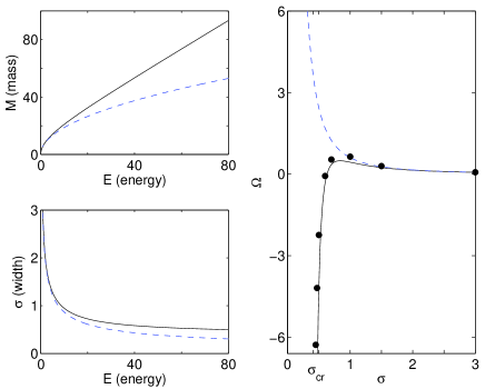
Figure 1: (color online) The left panels show the dependency of the mass $M$ (top) and the width $\sigma$ (bottom) on the chemical potential $E$. Black curves show results from the variational approach including local repulsion, dashed blue curves are without contact interaction. The right panel shows the angular frequency $\Omega$ as a function of $\sigma$. Black dots denote results obtained from numerical simulations of the GPE (1). All plots are for $p=0.7$.

As we observe in Fig. 1, the mass behaves like $\sqrt{E}$ close to $E=0$ , since generally, $M\sim A^{2}\sigma^{5}$, and for $\sigma\rightarrow\infty$, one finds $E\sim 1/\sigma^{2}$ $M\sim 1/\sigma$, whereas for $\sigma\rightarrow 0$, one finds $E\sim 1/\sigma^{2}$, $M\sim\sigma$. The fact that the mass can become zero for $E\rightarrow 0$ is a well-known property for very long range kernels, such as the Coulomb potential in three dimensions Fröhlich et al. (2002). For shorter ranged responses (e.g., Gaussian response, see Fig. 2), the mass attains its minimum at a finite value of $E$. In the limit of solely attractive local interaction ($E\rightarrow 0$, $\sigma\rightarrow\infty$), the mass is a monotonically decreasing function in $E$.

IV.2 The Gaussian response

Repeating each step of the previous calculations for the Gaussian nonlocal response, one ends up again with expressions for amplitude $A$ and rotation frequency $\Omega$, given by

$$A^{2}=\frac{\sqrt{2}\left(1+p^{2}\right)\left(\sigma^{2}+1\right)^{9/2}}{\frac{\left(9p^{4}+9+6p^{2}\right)\sigma^{13}}{160}+\frac{\left(4p^{2}+1+p^{4}\right)\sigma^{11}}{20}+\frac{\left(1+p^{2}\right)^{2}\sigma^{9}}{8}-\delta F_{\rm rep}}$$ (13)

with $F_{\rm rep}=(\sigma^{2}+1)^{9/2}(9p^{4}+9+6p^{2})\sigma^{4}/160$ and

$$\Omega=A^{2}\frac{p\left(\sigma^{7}-\delta(\sigma^{2}+1)^{7/2}\right)\sigma^{2}\sqrt{2}}{16(\sigma^{2}+1)^{7/2}}.$$ (14)

As already pointed out in Sec. II, the additional parameter $\delta$ is necessary due to an additional degree of freedom of the Gaussian response, and fixes the ratio between repulsion and attraction (see Appendix B). Obviously, for $\delta=0$, the repulsive local contact interaction vanishes. Here, $\sigma_{s}=\sqrt{\delta^{2/7}/\left(1-\delta^{2/7}\right)}\approx 0.60$ for $\delta=0.01$.

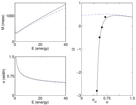
Figure 2: (color online) Same as Fig. 1, but for the Gaussian response given in Eq. (2). Black curves are for $\delta=0.01$, dashed blue curves without repulsion ($\delta=0.01$). All plots are for $p=0.7$.

We observe that $E\sim 1/\sigma^{2}$, $A\sim 1/\sigma^{2}$, $M\sim\sigma\sim 1/\sqrt{E}$ for both small and large $\sigma$. Compared to the ”gravitational” response, the range of this potential is much shorter. Hence, when considering large $\sigma$ the Gaussian response acts more and more like a local attractive response and higher order solitons become unstable (see end of Sec. V).

V Numerical results

In this section, the predictions of the variational approach will be confronted with direct numerical simulations. The approximate solitons resulting from the variational approach will be used as an initial conditions to our three-dimensional code to compute their time evolution. In general, we find stable evolution, in particular the characteristic shape of the initial conditions is preserved. For rotating azimuthons, the angular velocities will be measured and compared to the ones obtained in the previous section.

In Fig. 3 we illustrate the temporal evolution of three-dimensional solitons for the ”gravitational” response, i.e., solutions to Eq. (1). This first two rows present the classical stationary soliton solutions torus and dipole, respectively. Due to imperfections of the initial conditions obtained from the variational approach we observe slight oscillations upon evolution, in particular for the dipole solutions (second row). Those oscillations are not present if we use numerically exact solutions (obtained from an iterative solver Skupin et al. (2006)) as initial conditions (not shown). In the last row of Fig. 3 we show the evolution of an azimuthon ($p=0.7,\sigma=1$). The rotation of the amplitude profile is clearly visible. Again we observe radial oscillations due to the imperfect initial condition, but the solution is robust.

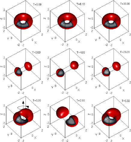
Figure 3: (color online) Dynamics of the three-dimensional stable solitons in gravity-like BEC. Iso-surfaces of the normalized density $\left|\psi\right|^{2}$ are depicted for different evolution times, the interior density distribution is represented in grey-scales. The initial variational parameters used are $\sigma=1$ and $p=1$ (torus, iso-density surface at $\left|\psi\right|^{2}=0.76$) for the upper row, $p=0$ (dipole, iso-density surface at $\left|\psi\right|^{2}=1.41$) for the middle one and finally $p=0.7$ (azimuthon, iso-density surface at $\left|\psi\right|^{2}=0.86$). The sense of the rotation ($\Omega=0.64$) is indicated by the arrows.

Figure 4 shows the dependency of the azimuthon rotation frequency as a function of the modulation parameter $p$. Solid lines represent predictions from the variational model, black dots represent rotation frequency obtained from numerical simulations. As expected from two-dimensional nonlocal models Lopez-Aguayo et al. (2006); Skupin et al. (2008), the modulus of $\Omega$ increases with $p$. Our variational calculations predict that for small width $\sigma$, when repulsive interaction comes into play, the sense of azimuthon rotation changes. In particular, we found a ”stationary” width $\sigma_{s}$ where the rotation frequency $\Omega$ vanishes. Indeed, full model simulations confirm this property, since the first row in Fig. 5 and  4, a) show a very slow rotation with opposite orientation, so that the numerical stationary width is between $0.6\dots 0.61$. Hence, we propose that tuning the strength of contact interaction in experiments allows to control the azimuthon rotation.

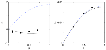
Figure 4: (color online) Azimuthon rotation frequency $\Omega$ vs modulation parameter $p$ in gravity-like BEC, for $\sigma=0.6\approx\sigma_{s}$ (left panel) and $\sigma=3$ (right panel). Black curves show results from the variational approach including local repulsion, dashed blue curves are without contact interaction. Black dots denote results obtained from numerical simulations of the GPE (1).

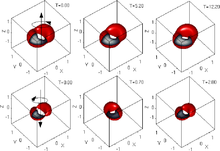
Figure 5: (color online) The upper row shows iso-density surfaces at $\left|\psi\right|^{2}=7.63$ for the very slow rotating ($\Omega\approx 0$) azimuthon with $p=0.7$ and $\sigma=0.61$. The lower row shows a fast counter-rotating ($\Omega=-2.24$) azimuthon with $p=0.7$, $\sigma=0.5$ and iso-density surface at $\left|\psi\right|^{2}=32$. Same plot style as in Fig. 3.

Furthermore, we observe that very narrow azimuthons ($\sigma\rightarrow\sigma_{cr}$) have negative $\Omega$ and rotate very fast (see Fig. 1). This may be interesting for potential experiments, since the duration of BEC experiments is restricted to typically several hundreds of milliseconds. However, for azimuthons very close to $\sigma_{cr}$ the ansatz function 7 becomes less appropriate and using variational initial conditions leads to very strong oscillations upon evolution, up to the point where is is no longer possible to identify properly the rotation frequency $\Omega$.

Concerning the Gaussian nonlocal response, we find very similar evolution scenarios. Results shown in the left panel in Fig. 6 for the Gaussian response underline the observations from above, in particular we also find nonrotating azimuthons at $\sigma=\sigma_{s}$. However, there are some important differences. First, it seems that our ansatz Eq. 7 is better suited for the Gaussian response, the radial oscillations we observed with the ”gravitational” are still present, but much weaker. The second difference is due to the fact that the Gaussian response has a much shorter range than the ”gravitational” one. For large $\sigma$ the Gaussian kernel acts like a attractive local response. As a consequence, higher order solitons become unstable in the sense that the two humps spiral out. We observe unstable evolution in numerical simulations for $\sigma\gtrsim 0.9$ at $p=0.7$. The right panel in Fig. 6 visualizes the cause of this instability: For increasing sigma the resulting convolution term $\Theta$ [Eq. (2)], which is responsible for the self-trapping, becomes smaller in amplitude and asymmetric in the rotation plane, which eventually leads to destabilization of the azimuthon.

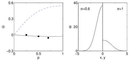
Figure 6: (color online) Azimuthon rotation frequency $\Omega$ vs modulation parameter $p$ in BEC with solely attractive Gaussian nonlocal response for $\sigma=0.6\approx\sigma_{s}$ (left panel). Black curves show results from the variational approach including local repulsion ($\delta=0.01$), dashed blue curves are without contact interaction ($\delta=0$). Black dots denote results obtained from numerical simulations (Eq. 2, $\delta=0.01$). The right panel shows profiles of the convolution term $\Theta$ [Eq. (2)] for $\sigma=0.6$ and $\sigma=1$. Solid lines correspond to profiles along the major axis of the resulting ellipsiod ($z=0$, $\varphi=0$), dotted lines to those along the minor axis ($z=0$, $\varphi=\pi/2$).

VI Conclusion

We studied formation of rotating localized structures in Bose Einstein condensate with different nonlocal interaction potentials. We successfully used variational techniques to investigate their dynamics and showed numerically that such localized structures are indeed robust objects which persist over long evolution times even if the initial conditions significantly differ from the exact soliton solutions.

For rotating solitons (azimuthons), we derived analytical expressions for the angular velocity, in excellent agreement with rigorous three-dimensional numerical simulations. Furthermore, we show that it is possible to control the rotation frequency by tuning the local contact interaction, which is routinely possible by Feshbach resonance techniques. In particular, we can change the sense of rotation, and we can find non-rotating azimuthons. We also identify parameter regions with particularly fast rotation, which may be important for potential experimental observation of such solutions.

By using different nonlocal kernel functions we showed that rotating soliton solutions are generic structures in nonlocal GPE’s. Hence, we conjecture that the phenomena observed in this paper are rather universal and apply for a general class of attractive nonlocal interaction potentials.

Appendix A normalization of the ”gravitational” model

We consider a Bose-Einstein atomic condensate with isotropic interatomic potential consisting with both, repulsive contact as well as attractive long-range nonlocal interaction contributions. Following O’Dell et.al O’Dell et al. (2000) the attractive long-range interaction which is electro-magnetically induced by the triads of frequency detuned laser beams with the intensity $I$ can be presented in the ”gravitational“ form

$$U_{Gr}\left(\tilde{\mathbf{r}}\right)=-\frac{11}{4\pi}\frac{Iq^{2}\alpha^{2}}{c\epsilon_{0}}\frac{1}{\tilde{r}}=-\frac{u}{\tilde{r}}$$ (15)

Here, $q$ is the modulus of the wave vector, $\alpha$ the isotropic, dynamic polarizability of the atoms, $c$ the light velocity and $\epsilon_{0}$ the permittivity of the free space. Then the complete two-body interaction potential is given by

$$V\left(\tilde{\mathbf{r}}\right)=\frac{4\pi a\hbar^{2}}{m}\delta\left(\tilde{\mathbf{r}}\right)-\frac{u}{\tilde{r}},$$ (16)

where the first term comes from the contact s-wave scattering, $a$ is the scattering length, and $m$ is the atomic mass. The potential can only be written in this form, if the mean kinetic energy per particle dominates the $u/\tilde{r}$-term, so that the short-range hard-sphere scattering is not affected. This is fulfilled, if $a_{B}\ll\lambda_{B}\ll a$, where $a_{B}:=\frac{h^{2}}{mu}$ is the Bohr radius, associated with the interaction, and $\lambda_{B}$ is the de Broglie wavelength.

The temporal and spatial dynamics of the condensate wave function $\tilde{\psi}\left(\mathbf{\tilde{r}},\tilde{t}\right)$ is then governed by the the following Gross-Pitaevskii equation (GPE):

$$\begin{split}\!\!i\hbar\partial_{\tilde{t}}\tilde{\psi}+\frac{\hbar^{2}}{2m}\Delta_{\tilde{\mathbf{r}}}\tilde{\psi}+u\int\frac{\left|\tilde{\psi}\left(\tilde{\mathbf{r}}^{\prime},\tilde{t}\right)\right|^{2}}{\left|\tilde{\mathbf{r}}-\tilde{\mathbf{r}}^{\prime}\right|}d^{3}\tilde{\mathbf{r}}^{\prime}\tilde{\psi}&\\ -\frac{4\pi a\hbar^{2}}{m}\left|\tilde{\psi}\right|^{2}\tilde{\psi}&=0.\end{split}$$ (17)

Using the normalization

$$\psi :=\sqrt{8\pi aR_{c}^{2}}\tilde{\psi}=:\frac{1}{\psi_{c}}\tilde{\psi}$$ (18a)

$$\mathbf{r} :=\sqrt{\frac{um}{4\pi a\hbar^{2}}}\tilde{\mathbf{r}}=:\frac{1}{R_{c}}\tilde{\mathbf{r}}$$ (18b)

$$t :=\frac{\hbar}{2mR_{c}^{2}}\tilde{t}=:\frac{1}{T_{c}}\tilde{t},$$ (18c)

one ends up with the dimensionless GPE (1). The actual values for the scaling parameters are $R_{c}=19\mu m$, $m=3.8\cdot 10^{-26}\mathrm{kg}$, $a=3nm$, $u=2\cdot 10^{-13}eVnm$, $T{}_{c}=0.25s$ which corresponds to typical experimental conditions O’Dell et al. (2000). Then one finds that for the condensate consisting of, say, $N=10000$ atoms the above normalization gives

$$M=\int\left|\psi\right|^{2}\mathrm{d}^{3}\mathbf{r}=\frac{N}{\psi_{c}^{2}R_{c}^{3}}\approx{42}.$$ (19)

Appendix B normalization for the Gaussian model

For the Gaussian response, one has to start from the equation

$$\begin{split}i\hbar\partial_{\tilde{t}}\tilde{\psi}+\frac{\hbar^{2}}{2m}\Delta\tilde{\psi}-\frac{4\pi a\hbar^{2}}{m}\left|\tilde{\psi}\right|^{2}\tilde{\psi}&\\ +A_{R}\int\left|\tilde{\psi}\left(\tilde{\mathbf{r}}^{\prime},\tilde{t}\right)\right|^{2}e^{-\frac{\left|\tilde{\mathbf{r}}-\tilde{\mathbf{r}}^{\prime}\right|^{2}}{2\sigma_{R}^{2}}}\mathrm{d}^{3}\tilde{\mathbf{r}}^{\prime}\tilde{\psi}&=0\end{split}$$ (20)

Here, the degree of nonlocality (i.e. $\sigma_{R}$), that is fixed for the $1/r$-response, and the amplitude $A_{R}$ of the the response function can be chosen. By using the normalization

$$\psi :=\frac{1}{4}\frac{\hbar 2^{3/4}}{\sigma^{2}\pi^{3/4}\sqrt{A_{R}\sigma m}}=:\frac{1}{\psi_{c}}\tilde{\psi}$$ (21a)

$$\mathbf{r} :=\sigma_{R}\tilde{\mathbf{r}}=:\frac{1}{R_{c}}\tilde{\mathbf{r}}$$ (21b)

$$t :=\frac{2\sigma^{2}m}{\hbar}\tilde{t}=:\frac{1}{T_{c}}\tilde{t}$$ (21c)

$$\delta :=\frac{a\hbar^{2}\sqrt{2}}{\sigma_{R}^{3}\sqrt{\pi}mA_{R}},$$ (21d)

one ends up with Eq. 2, that has the additional degree of freedom $\delta$.

Appendix C convolution

The convolution term in the Lagrangian (6) can be calculated analytically by, for instance, re-writing the integrand in terms of spherical harmonics $Y_{ij}$. Then, $\left|\psi\left(\mathbf{r}\right)\right|^{2}=\sum y_{ij}Y_{ij}$, where $y_{ij}$ denote the coefficients of the spherical harmonics, and the convolution integral can be easily calculated leading to the following result:

$$\frac{1}{2}\int\left|\psi\left(\mathbf{r}\right)\right|^{2}\int\frac{\left|\psi\left(\mathbf{r}^{\prime}\right)\right|^{2}}{\left|\mathbf{r}-\mathbf{r}^{\prime}\right|}d^{3}\mathbf{r}^{\prime}d^{3}\mathbf{r}$$

$$= \frac{1}{2}\int_{0}^{\infty}\int_{0}^{r}4\pi rA^{4}r^{\prime 2}\exp\left(-\frac{r^{\prime 2}+r^{2}}{\sigma^{2}}\right)$$

$$\times\left(y_{00}^{2}+\frac{1}{5}y_{20}^{2}\left(\frac{r^{\prime}}{r}\right)^{2}+\frac{2}{5}y_{2\pm 2}^{2}\left(\frac{r^{\prime}}{r}\right)^{2}\right)r^{\prime 2}\mathrm{d}r^{\prime}r^{2}\mathrm{d}r$$

$$+\frac{1}{2}\int_{0}^{\infty}\int_{r}^{\infty}4\pi r^{\prime}A^{4}r^{2}\exp\left(-\frac{r^{\prime 2}+r^{2}}{\sigma^{2}}\right)$$

$$\times\left(y_{00}^{2}+\frac{1}{5}y_{20}^{2}\left(\frac{r}{r^{\prime}}\right)^{2}+\frac{2}{5}y_{2\pm 2}^{2}\left(\frac{r}{r^{\prime}}\right)^{2}\right)r^{\prime 2}\mathrm{d}r^{\prime}r^{2}\mathrm{d}r$$

$$= \frac{49+86p^{2}+49p^{4}}{240}\sigma^{9}\pi^{\frac{5}{2}}A^{4}\frac{1}{\sqrt{2}}.$$

References

- Giorgini et al. (2008) S. Giorgini, L. P. Pitaevskii, and S. Stringari, Rev. Mod. Phys. 80, 1215 (2008).
- Bloch et al. (2008) I. Bloch, J. Dalibard, and W. Zwerger, Rev. Mod. Phys. 80, 885 (2008).
- Dalfovo et al. (1999) F. Dalfovo, S. Giorgini, L. P. Pitaevski, and S. Stringari, Rev. Mod. Phys. 71, 463 (1999).
- Khaykovich et al. (2002) L. Khaykovich, F. Schreck, G. Ferrari, T. Bourdel, J. Cubizolles, L. D. Carr, Y. Castin, and C. Salomon, Science 296, 1290 (2002).
- Strecker et al. (2002) K. E. Strecker, G. B. Partridge, A. G. Truscott, and R. G. Hulet, Nature London 417, 150 (2002).
- Goral et al. (2000) K. Goral, K. Rzazewski, and T. Pfau, Phys. Rev. A 61, 051601(R) (2000).
- Beaufils et al. (2008) Q. Beaufils, R. Chicireanu, T. Zanon, B. Laburthe-Tolra, E. Maréchal, L. Vernac, J.-C. Keller, and O. Gorceix, Phys. Rev. A 77, 061601(R) (2008).
- Griesmaier et al. (2005) A. Griesmaier, J. Werner, S. Hensler, J. Stuhler, and T. Pfau, Phys. Rev. Lett. 94, 160401 (2005).
- Stuhler et al. (2005) J. Stuhler, A. Griesmaier, T. Koch, M. Fattori, T. Pfau, S. Giovanazzi, P. Pedri, and L. Santos, Phys. Rev. Lett. 95, 150406 (2005).
- Lahaye et al. (2007) T. Lahaye, T. Koch, B. Fröhlich, M. Fattori, J. Metz, A. Griesmaier, S. Giovanazzi, and T. Pfau, Nature (London) 448, 672 (2007).
- Koch et al. (2008) T. Koch, T. Lahaye, J. Metz, B. Fröhlich, A. Griesmaier, and T. Pfau, Nat. Phys. 4, 218 (2008).
- Pedri and Santos (2005) P. Pedri and L. Santos, Phys. Rev. Lett. 95, 200404 (2005).
- Pollack et al. (2009) S. E. Pollack, D. Dries, M. Junker, Y. P. Chen, T. A. Corcovilos, and R. G. Hulet, Phys. Rev. Lett. 102, 090402 (2009).
- Bang et al. (2002) O. Bang, W. Krolikowski, J. Wyller, and J. J. Rasmussen, Phys. Rev. E 66, 046619 (2002).
- Nath et al. (2007) R. Nath, P. Pedri, and L. Santos, Phys. Rev. A 76, 013606 (2007).
- Cuevas et al. (2009) J. Cuevas, B. A. Malomed, P. G. Kevrekidis, and D. J. Frantzeskakis, Phys. Rev. A 79, 053608 (2009).
- Lashkin (2007) V. M. Lashkin, Phys. Rev. A 75, 043607 (2007).
- Lashkin (2008) V. M. Lashkin, Phys. Rev. A 78, 033603 (2008).
- Zaliznyak and Yakimenko (2008) Y. A. Zaliznyak and A. I. Yakimenko, Phys. Lett. A 372, 2862 (2008).
- Lashkin et al. (2009) V. M. Lashkin, A. L. Yakimenko, and Y. A. Zaliznyak, Phys. Scr. 79, 035305 (2009).
- Nath et al. (2008) R. Nath, P. Pedri, and L. Santos, Phys. Rev. Lett. 101, 210402 (2008).
- O’Dell et al. (2000) D. S. O’Dell, S. Giovanazzi, G. Kurizki, and V. M. Akulin, Phys. Rev. Lett. 84, 5687 (2000).
- Turitsyn (1985) S. K. Turitsyn, Theor, Mat. Fiz. 64, 797 (1985).
- Giovanazzi et al. (2001) S. Giovanazzi, D. O’Dell, and G. Kurizki, Phys. Rev. A 63, 031603(R) (2001).
- Papadopoulos et al. (2007) I. Papadopoulos, P. Wagner, G. Wunner, and J. Main, Phys. Rev. A 76, 053604 (2007).
- Cartarius et al. (2008) H. Cartarius, T. Fabcic, J. Main, and G. Wunner, Phys. Rev. A 78, 013615 (2008).
- Keles et al. (2008) A. Keles, S. Sevincli, and B. Tanatar, Phys. Rev. A 77, 053604 (2008).
- Krolikowski et al. (2004) W. Krolikowski, N. Nikolov, D. Neshev, O. Bang, J. J. Rasmussen, and J. Wyller, J. Opt. B. 6, 288 (2004).
- Buccoliero et al. (2007a) D. Buccoliero, S. Lopez-Aguayo, S. Skupin, A. Desyatnikov, O. Bang, W. Krolikowski, and Y. S. Kivshar, Physica B 394, 351 (2007a).
- Skupin et al. (2008) S. Skupin, M. Grech, and W. Krolikowski, Opt. Express 16, 9118 (2008).
- Buccoliero et al. (2007b) D. Buccoliero, A. S. Desyatnikov, W. Krolikowski, and Y. S. Kivshar, Phys. Rev. Lett. 98, 053901 (2007b).
- Ginibre and Velo (1980) J. Ginibre and G. Velo, Mathematische Zeitschrift 170, 109 (1980).
- Fröhlich et al. (2002) J. Fröhlich, T. Tsai, and H. Yau, Communications in Mathematical Physics 225, 223 (2002).
- Skryabin et al. (2002) D. V. Skryabin, J. M. McSloy, and W. J. Firth, Phys. Rev. E 66, 055602(R) (2002).
- Desyatnikov et al. (2005) A. S. Desyatnikov, A. A. Sukhorukov, and Y. S. Kivshar, Phys. Rev. Lett. 95, 203904 (2005).
- Rozanov (2004) N. N. Rozanov, Opt Spectrosc 96, 405 (2004).
- Malomed (2002) B. A. Malomed, Prog. Opt. 43, 71 (2002).
- Skupin et al. (2006) S. Skupin, O. Bang, D. Edmundson, and W. Krolikowski, Phys. Rev. E 73, 066603 (2006).
- Lopez-Aguayo et al. (2006) S. Lopez-Aguayo, A. Desyatnikov, Y. S. Kivshar, S. Skupin, W. Krolikowski, and O. Bang, Opt. Lett 31, 1100 (2006).