Quantum manipulation in a Josephson LED

Abstract

We access the suitability of the recently proposed Josephson LED for quantum manipulation purposes. We show that the device can both be used for on-demand production of entangled photon pairs and operated as a two-qubit gate. Besides, one can entangle particle spin with photon polarization and/or measure the spin by measuring the polarization.

1 Introduction

It is tempting to use the advantages of semiconductors and superconductors, combined within a single nanodevice, for quantum manipulation purposes. Making such combined nanostructures turned out to be a difficult technological problem and a lot of experimental effort has been concentrated on this direction [1]. Progress has been achieved with semiconductor nanowires: Superconducting field-effect transistor [2] and Josephson effect [3, 4] in a semiconducting quantum dot have been experimentally confirmed. Recently, a next step has been made. It was proposed to combine semiconducting quantum dots and superconducting leads to make a Josephson LED where the light-emission ability of a semiconductor is enhanced by the intrinsic coherence of the superconducting state [5].

Semiconducting quantum dots exhibit narrow emission lines and quasi-atomic discrete states, this enables quantum applications involving visible photons. The optical emission shows close to perfect photon antibunching [6, 7, 8], so the dots can be used as single-photon emitters. Rabi oscillations [9] and coherent manipulation of excitons (electron-hole bound states) have been demonstrated [10]. Furthermore, the possibility of controlled charging with extra carriers [11] allows the use of single electron [12, 13] or hole [14, 15] spins that exhibit ultra-long spin-coherence times [16]. Importantly, biexciton cascades, which are sources of photon pairs emitted sequentially [17], were proposed to generate polarization entangled photons [18, 19]. However, the exchange splitting of a single exciton due to asymmetric dots renders the two possible circular polarizations nondegenerate and hinders the observation of entanglement [20]. This problem can be overcome by improvements in the sample design [21] or by spectral filtering [22]. A more serious disadvantage is the use of incoherent transitions to prepare a biexcitation. Owing to this, it is hard if possible at all to generate entangled pairs on demand, a functionality that is required in most quantum algorithms [23].

In this article, we address the rich potential of the newly proposed Josephson LED for quantum manipulation purposes. We show how to operate the device for on-demand production of entangled photon pairs. We demonstrate that Josephson LEDs may be used as a two-qubit quantum gates. Moreover, we show how to entangle the spin of a particle in one of the quantum dots with the polarization of an emitted photon. We also outline an alternative scheme to measure the spin of the particle via the conversion of the spin into the polarization of a photon.

2 Setup

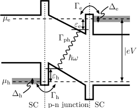
Figure 1: Level diagram of the double quantum dot in a p-n junction where each side is coupled to a superconducting lead with pairing amplitude $\Delta_{\rm h,e}$. The levels are detunes by $\varepsilon_{\rm h,e}$ with respect to the chemical potential $\mu_{\rm h,e}$ on either side. The coupling to the superconducting leads introduces coherent transfer of Cooper pairs changing the occupation number of the dot by 2. The p-n junction is biased with a voltage $V$ which sets the energy scale of electron-hole recombination via the emission of photons at frequency $\omega=|eV|/\hbar$.

The setup of the Josephson light emitting diode (JoLED) was outlined in detail in [5]. It consists of a p-n junction in a semiconducting wire where either side features a quantum dot. Each quantum dot can incorporate up to two holes (h) or electrons (e) in a single level. The potential barriers are arranged to assure that the only process of charge transfer through the junction is the recombination of an electron and a hole in the dots. The p-n junction is biased with a voltage $V$. This sets the energy scale $|eV|$ for photons emitted via recombination of a electron and a hole at a rate $\Gamma_{\rm ph}$. Either dot is coupled to a superconducting lead with a pairing amplitude $\Delta_{\rm h,e}=|\Delta_{\rm h,e}|\exp(i\phi_{\rm h,e})$. Thereby, each superconducting lead introduces mixing between the empty and the doubly occupied state of the dots via the proximity effect; we denote by $\tilde{\Delta}_{\rm h,e}=(\Gamma_{\rm h,e}/2)\exp(i\phi_{\rm h,e})$ the induced paring amplitude on the dots with $\Gamma_{\rm h,e}$ the level broadening proportional to the square of the amplitude to tunnel an electron from the dot to the superconducting lead. The Hamiltonian $H=H_{\rm d}+H_{\rm m}$ of the system consists of two terms. The first term

$$H_{\rm d}=\varepsilon_{\rm h}n_{\rm h}+U_{\rm h}n_{\rm h}(n_{\rm h}-1)+\varepsilon_{\rm e}n_{\rm e}+U_{\rm e}n_{\rm e}(n_{\rm e}-1)+U_{\rm he}n_{\rm h}n_{\rm e}$$ (1)

is diagonal in the charge basis with $n_{\rm h}$ ($n_{\rm e}$) being the number of holes (electrons); here, $\varepsilon_{\rm h}$ ($\varepsilon_{\rm e}$) denotes the level of the dot with respect to the chemical potential $\mu_{\rm h}$ ($\mu_{\rm e}$) in the p (n) region, $U_{\rm h,e}$ denotes the on-site charging energy and $U_{\rm he}$ is the Coulomb interaction between the carriers in the dots. The effect of $U_{\rm he}$ has not been considered in [5] and is an important detail of our setup. The second term (due to the superconducting leads)

$$H_{\rm m}=\tilde{\Delta}_{\rm h}|2_{\scriptscriptstyle\rm h}\rangle\langle 0_{\scriptscriptstyle\rm h}|+\tilde{\Delta}_{\rm e}|2_{\scriptscriptstyle\rm e}\rangle\langle 0_{\scriptscriptstyle\rm e}|+{\rm H.c.},$$ (2)

introduces mixing between states with well-defined charge; here and in the following, $|n_{\scriptscriptstyle\rm h}\rangle$ ($|n_{\scriptscriptstyle\rm e}\rangle$) denotes the state with n holes (electrons) on the left (right) dot. In [5], a general case $\tilde{\Delta}\simeq U$ has been considered so that the mixing between the charge states has been always essential. Here, we are interested in a limit where $\tilde{\Delta}\ll U\ll\Delta$, i.e., expression (1) is typically the dominant term in the Hamiltonian and (2) constitutes a perturbation.

In this limit, quantum manipulation functionality is enabled. The Hamiltonian $H_{\rm d}$ without mixing naturally constitutes a two qubit system with the four states given by $|0_{\scriptscriptstyle\rm h}0_{\scriptscriptstyle\rm e}\rangle$, $|2_{\scriptscriptstyle\rm h}0_{\scriptscriptstyle\rm e}\rangle$, $|0_{\scriptscriptstyle\rm h}2_{\scriptscriptstyle\rm e}\rangle$, $|2_{\scriptscriptstyle\rm h}2_{\scriptscriptstyle\rm e}\rangle$, and the two qubits correspond to the two different dots. We note that the qubits interact with each other, since $U_{he}$ is nonzero. For instance, the energy difference between $|0_{\scriptscriptstyle\rm e}\rangle$ and $|2{\scriptscriptstyle\rm e}\rangle$ depends on number of holes in the neighboring hole dot. This offers the possibility to operate two qubit gates [24].

3 Dynamics without manipulation

Figure 2: Scheme of the 9 states (without spin degree of freedom) of the double quantum dot and possible transitions due to electron-hole recombination (wavy lines). As the recombination annihilates one electron with one hole these processes cannot change the parity of the total number of electrons and holes on the dots. Therefore, the diagram is separated into two parts: At the top, there are the even parity states and on the bottom the odd ones. The dashed lines indicate possible two particle transfers which can happen due to the nearby superconductors. Note that these processes only contribute with an appreciable probability when the involved states are nearly degenerate in energy.

At first, we describe the dynamics of JoLED without manipulation. As noted above, the mixing of different charge state is small and thus we neglect it at the moment. We will comment on the effect of mixing at the end of the section. The coupling of the states of the dot to the radiation field leads to emission of photons with frequency $\omega\approx|eV|/\hbar$. The system we have in mind is a III-V semiconductor, e.g., GaAs or InAs, where the electrons in the conduction band carry a spin $\pm 1/2$ while the holes in the valence band carry a total angular momentum $3/2$. Following the basic assumptions about spin-polarization conversion in quantum wells, we take for granted that the angular momentum and spin of a dot state are in the same direction [25]. This gives the following selection rule: The recombination is only possible for electron and hole of the same spin ($\uparrow$ or $\downarrow$) and produces a photon of circular polarization corresponding to the direction of this spin ($+$ or $-$). The recombination of the states $|{\uparrow}_{\scriptscriptstyle\rm h}{\downarrow}_{\scriptscriptstyle\rm e}\rangle$ and $|{\downarrow}_{\scriptscriptstyle\rm h}{\uparrow}_{\scriptscriptstyle\rm e}\rangle$ is forbidden by the selection rule and happens with a much smaller rate. Assuming an appropriate spin configuration, the decay channels are depicted by wavy lines in figure 2. We note that the parity of the total number of electrons and holes is conserved by the process of photon emission: The parity is even in the top and odd in the bottom cycle in the figure. If initially the JoLED is in the state $|2_{\scriptscriptstyle\rm h}2_{\scriptscriptstyle\rm e}\rangle$ or $|1_{\scriptscriptstyle\rm h}1_{\scriptscriptstyle\rm e}\rangle$, it will be in the state $|0_{\scriptscriptstyle\rm h}0_{\scriptscriptstyle\rm e}\rangle$ after a time $\simeq\Gamma_{\rm ph}^{-1}$. Similarly, it will be in $|0_{\scriptscriptstyle\rm h}1_{\scriptscriptstyle\rm e}\rangle$ or $|1_{\scriptscriptstyle\rm h}0_{\scriptscriptstyle\rm e}\rangle$ if the initial parity is odd.

There are secondary (slow) processes not depicted in figure 2 that change the parity. These processes emit photons together with the creation of a quasiparticle in one of the superconducting leads and therefore connect the even- and odd-parity cycles in figure 2. As an example, consider the case where the initial state is given by $|1_{\scriptscriptstyle\rm h}0_{\scriptscriptstyle\rm e}\rangle$. In a virtual process, an electron can tunnel in from the superconductor on the electron side such that the dots are now in the (intermediate) state $|1_{\scriptscriptstyle\rm h}1_{\scriptscriptstyle\rm e}\rangle$ leaving behind a quasiparticle with energy larger than $|\Delta_{\rm e}|$ in the lead, followed by the emission of a photon such that the dots end up in the state $|0_{\scriptscriptstyle\rm h}0_{\scriptscriptstyle\rm e}\rangle$. The (typical) rate for this secondary emission is given by $\tilde{\Gamma}_{\rm ph;e}\simeq\Gamma_{\rm ph}\Gamma_{\rm e}/|\Delta_{\rm e}|$ which is smaller by $|\tilde{\Delta}_{\rm e}/\Delta_{\rm e}|\ll 1$ than the primary emission; a similar process going from $|0_{\scriptscriptstyle\rm h}1_{\scriptscriptstyle\rm e}\rangle$ to $|0_{\scriptscriptstyle\rm h}0_{\scriptscriptstyle\rm e}\rangle$ via the creation of a quasihole in the superconducting lead on the p-side has a typical rate $\tilde{\Gamma}_{\rm ph;h}\simeq\Gamma_{\rm ph}\Gamma_{\rm h}/|\Delta_{\rm h}|$. Taking both the primary and secondary photon emission processes into account, we come to the following conclusion: The JoLED will end up in the ground state $|0_{\scriptscriptstyle\rm h}0_{\scriptscriptstyle\rm e}\rangle$ after time $\simeq\Gamma_{\rm ph;e,h}^{-1}$. This proves that the two-quit gate is automatically prepared in the initial state $|0_{\scriptscriptstyle\rm h}0_{\scriptscriptstyle\rm e}\rangle$. The effect of a small nonvanishing mixing $\tilde{\Delta}$ is now easily discussed resorting to perturbation theory. In fact the state $|0_{\scriptscriptstyle\rm h}0_{\scriptscriptstyle\rm e}\rangle$ is not an eigenstate of the system and the true ground state has also components $|2_{\scriptscriptstyle\rm h}0_{\scriptscriptstyle\rm e}\rangle$, $|0_{\scriptscriptstyle\rm h}2_{\scriptscriptstyle\rm e}\rangle$, and $|2_{\scriptscriptstyle\rm h}2_{\scriptscriptstyle\rm e}\rangle$ admixed. Those states however are generically detuned from the state $|0_{\scriptscriptstyle\rm h}0_{\scriptscriptstyle\rm e}\rangle$ by $U$. Therefore, the amplitude to be in state $|2_{\scriptscriptstyle\rm h}2_{\scriptscriptstyle\rm e}\rangle$ is given by $\tilde{\Delta}_{\rm e}\tilde{\Delta}_{\rm h}/U^{2}$ in second order perturbation theory in $H_{\rm m}$ and the probability to be in state $|2_{\scriptscriptstyle\rm h}2_{\scriptscriptstyle\rm h}\rangle$ which can decay via the recombination of excitons reads $|\tilde{\Delta}_{\rm e}|^{2}|\tilde{\Delta}_{\rm h}|^{2}/U^{4}\ll 1$. For that reason, including mixing thus does not change our conclusion. The system remains in the ground state $|0_{\scriptscriptstyle\rm h}0_{\scriptscriptstyle\rm e}\rangle$ with overwhelming probability.

4 On-demand production of photon pairs

So far, we were only considering the states of the Hamiltonian (1) together with the coupling to the radiation field. In a next step, we introduce mixing given by (2). Mixing provides a coherent coupling between the eigenstates of $H_{\rm q}$ depicted by dashed lines in figure 2. At first, we are interested in the case where figure 2 contains a closed cycle such that a constant stream of photons is produced. This can be achieved by tuning the on-site energies $\varepsilon_{\rm h,e}$ via voltages of close-by gates. Having two tuning parameters, we can activate two mixing processes by tuning the relevant eigenstates into degeneracy. We know that $|0_{\scriptscriptstyle\rm h}0_{\scriptscriptstyle\rm e}\rangle$ is the equilibrium state without mixing. If we therefore tune this level into degeneracy with $|0_{\scriptscriptstyle\rm h}2_{\scriptscriptstyle\rm e}\rangle$ and $|2_{\scriptscriptstyle\rm h}2_{\scriptscriptstyle\rm e}\rangle$, the cycle $|0_{\scriptscriptstyle\rm h}0_{\scriptscriptstyle\rm e}\rangle\to|0_{\scriptscriptstyle\rm h}2_{\scriptscriptstyle\rm e}\rangle\to|2_{\scriptscriptstyle\rm h}2_{\scriptscriptstyle\rm e}\rangle\to|1_{\scriptscriptstyle\rm h}1_{\scriptscriptstyle\rm e}\rangle\to|0_{\scriptscriptstyle\rm h}0_{\scriptscriptstyle\rm e}\rangle$ becomes active in which two photons are produced with frequencies $\hbar\omega\approx eV$. This cycle is interrupted from time to time by a secondary photon emission which brings the system to the odd (bottom) cycle. There it remains for some time in one of the states $|1_{\scriptscriptstyle\rm h}0_{\scriptscriptstyle\rm e}\rangle$ or $|0_{\scriptscriptstyle\rm h}1_{\scriptscriptstyle\rm e}\rangle$ until the secondary photon emission brings it back to $|0_{\scriptscriptstyle\rm h}0_{\scriptscriptstyle\rm e}\rangle$. The degeneracy of the states can be obtained by setting the on-site energy levels to

$$\varepsilon^{*}_{\rm h}=-U_{\rm h}-2U_{\rm he}\qquad\varepsilon^{*}_{\rm e}=-U_{\rm e}.$$ (3)

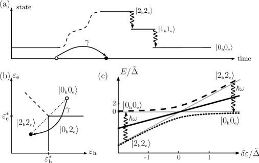
Figure 3: (a) Time-line depicting the pumping of the quantum dots (between the white and the black dot) together with the subsequent emission of two (entangled) photons. (b) Diagram showing which of the states $|0_{\scriptscriptstyle\rm h}0_{\scriptscriptstyle\rm e}\rangle$, $|0_{\scriptscriptstyle\rm h}2_{\scriptscriptstyle\rm e}\rangle$, $|2_{\scriptscriptstyle\rm h}2_{\scriptscriptstyle\rm e}\rangle$ has the lowest energy given a set of parameters $\varepsilon_{\rm h},\varepsilon_{\rm e}$. At the boundaries (solid and dashed lines), the bordering states are degenerate neglecting the mixing introduced by $H_{\rm m}$. The mixing induces an energy gap along the solid lines. Changing the state adiabatically from the white dot to the black dot along the path $\gamma$, we transfer the dot from the state $|0_{\scriptscriptstyle\rm h}0_{\scriptscriptstyle\rm e}\rangle$ to $|2_{\scriptscriptstyle\rm h}2_{\scriptscriptstyle\rm e}\rangle$. (c) Level scheme depicting the anticrossing of the three states along the dotted line in (a) where $\delta\varepsilon=\delta\varepsilon_{\rm h}=\delta\varepsilon_{\rm e}$ and $\tilde{\Delta}=|\tilde{\Delta}_{\rm h}|=|\tilde{\Delta}_{\rm e}|$. The cycle produces photon pairs on demand and is described in detail in the main text. We start with the dots in the ground state $|0_{\scriptscriptstyle\rm h}0_{\scriptscriptstyle\rm e}\rangle$ at $\delta\varepsilon>\tilde{\Delta}$. Adiabatically changing $\delta\varepsilon$ to $\delta\varepsilon<-\tilde{\Delta}$, we drive the levels through the anticrossing and end up with the state $|2_{\scriptscriptstyle\rm h}2_{\scriptscriptstyle\rm e}\rangle$ which relaxes to $|0_{\scriptscriptstyle\rm h}0_{\scriptscriptstyle\rm e}\rangle$ via the emission of an entangled pair of photons. Changing $\delta\varepsilon$ adiabatically back to the original situation, an additional pair of photons is produced leading to a total of two photon pairs per cycle in the $\varepsilon_{\rm h,e}$ parameter space.

Close to the degeneracy point $\varepsilon_{h,e}^{*}$, the states $|0_{\scriptscriptstyle\rm h}0_{\scriptscriptstyle\rm e}\rangle$, $|0_{\scriptscriptstyle\rm h}2_{\scriptscriptstyle\rm e}\rangle$, and $|2_{\scriptscriptstyle\rm h}2_{\scriptscriptstyle\rm e}\rangle$ are almost degenerate and the remaining 6 states are separated by the interaction energy $U$. The induced superconducting gaps lead to mixing of the dot states which can be used to excite the dot followed by photon emission. Denoting the detuning from the degeneracy point by $\delta\varepsilon_{\rm h,e}=\varepsilon_{\rm h,e}-\varepsilon_{\rm h,e}^{*}$, the Hamiltonian

$$H^{\prime}=\left(\begin{array}[]{ccc}0&\tilde{\Delta}_{\rm e}^{*}&0\\ \tilde{\Delta}_{\rm e}&2\,\delta\varepsilon_{\rm e}&\tilde{\Delta}_{\rm h}^{*}\\ 0&\tilde{\Delta}_{\rm h}&2\,\delta\varepsilon_{\rm h}+2\,\delta\varepsilon_{\rm e}\end{array}\right)$$ (4)

is almost degenerate in the subspace $\{|0_{\scriptscriptstyle\rm h}0_{\scriptscriptstyle\rm e}\rangle,|0_{\scriptscriptstyle\rm h}2_{\scriptscriptstyle\rm e}\rangle,|2_{\scriptscriptstyle\rm h}2_{\scriptscriptstyle\rm e}\rangle\}$. Figure 3(b) shows the parameter space $\varepsilon_{\rm h}$, $\varepsilon_{\rm e}$ together with the state which have to lowest energy for these parameters. At the boundaries, two of the states become degenerate. Along the solid line a gap opens due to mixing of the states caused by the superconductor so the level crossing becomes an anticrossing gapped by $|\tilde{\Delta}|$. Along the dashed line, no gap opens as the states involved are not coupled by the Hamiltonian (4). Starting from the ground state $|0_{\scriptscriptstyle\rm h}0_{\scriptscriptstyle\rm e}\rangle$ [denoted by the white dot in figure 3(b)] in the region $\delta e_{\rm h}>-\delta_{\rm e},\delta_{\rm e}>0$ and moving the state adiabatically along $\gamma$ via the state $|0_{\scriptscriptstyle\rm h}2_{\scriptscriptstyle\rm e}\rangle$ to the black dot in the region where $|2_{\scriptscriptstyle\rm h}2_{\scriptscriptstyle\rm e}\rangle$ is the lowest state of $H^{\prime}$, we end up with the state $|2_{\scriptscriptstyle\rm h}2_{\scriptscriptstyle\rm e}\rangle$ which will subsequently decay via the emission of two photons, cf. figure 2. Figure 3(c) shows the level scheme for the case when the states are tuned through the triple point along the dotted line in figure 3(b). The spectrum for paths which do go directly through the triple point are similar but feature two instead of one anticrossing. After the emission of the photons, we are back in the state $|0_{\scriptscriptstyle\rm h}0_{\scriptscriptstyle\rm e}\rangle$ which can be repumped into $|2_{\scriptscriptstyle\rm h}2_{\scriptscriptstyle\rm e}\rangle$ by retracing the path $\gamma$ thus completing the cycle. Note that the pumping should be slow in order to be adiabatic but fast such that the intermediate state $|0_{\scriptscriptstyle\rm h}2_{\scriptscriptstyle\rm e}\rangle$ does not decay due to secondary photon emission; this approximately translates into $\tilde{\Delta}^{-1}\ll t_{\rm pump}\ll\tilde{\Gamma}_{\rm ph}$ with $t_{\rm pump}$ the pumping time. Photons pairs can be produced at will by employing the adiabatic pumping. However, the photon emission process is stochastic in its nature and the exact time when the photons are produced cannot be controlled. Pumping the system, we obtain a pair of photons somewhere within the time $\Gamma_{\rm ph}^{-1}$.

Figure 4: (a) Biexciton cascade which leads to the generation of a pair of entangled photons. (b) For the production of spin-polarization entanglement, the process in (a) is interrupted after the first photon emission and the electron remaining in the dot is kicked out into the lead by a pulse in gate voltage $V_{\rm e}$.

The photons created in the cycle are entangled in their polarization degree on freedom. Starting with the state $\Psi_{0}=|2_{\scriptscriptstyle\rm h}2_{\scriptscriptstyle\rm e}\rangle$ of the dot immediately after pumping, the first photon which is emitted can either be $+$ or $-$ polarized. In fact, the state $\Psi_{1}$ after the first emission is a linear superposition of the photon being in state $|+_{\scriptscriptstyle\rm 1}\rangle$ or $|-_{\scriptscriptstyle\rm 1}\rangle$ with the same amplitude for both. After the first photon emission, the state of the system (dot and photon) reads

$$\Psi_{1}\propto|{\downarrow}_{\scriptscriptstyle\rm h}{\downarrow}_{\scriptscriptstyle\rm e}\rangle|+_{\scriptscriptstyle\rm 1}\rangle+|{\uparrow}_{\scriptscriptstyle\rm h}{\uparrow}_{\scriptscriptstyle\rm e}\rangle|-_{\scriptscriptstyle\rm 1}\rangle.$$ (5)

Note that the polarization of the photon is connected to the state of the remaining hole and electron. Therefore, the polarization of the photon produced in the second recombination is linked to the polarization of the first photon and we end up with the state

$$\Psi_{2}\propto|0_{\scriptscriptstyle\rm h}0_{\scriptscriptstyle\rm e}\rangle(|+_{\scriptscriptstyle\rm 1}-_{\scriptscriptstyle\rm 2}\rangle+|-_{\scriptscriptstyle\rm 1}+_{\scriptscriptstyle\rm 2}\rangle),$$ (6)

with the polarization degrees of freedom are (completely) entangled. The physics behind the polarization entanglement is the same as observed in biexciton cascade in semiconducting quantum dots without superconducting leads [21, 22]. However, the pumping scheme differs as the biexciton is electrostatically pumped without the need of an radiation field whereas traditionally the biexciton state $|2_{\scriptscriptstyle\rm h}2_{\scriptscriptstyle\rm e}\rangle$ is pumped with lasers via the single exciton state $|1_{\scriptscriptstyle\rm h}1_{\scriptscriptstyle\rm e}\rangle$ which is unstable itself and can decay such that the pumping has to be faster than the exciton decay time. The electrostatic pumping may ease the detection of the entangled photons as no background laser field is present.

5 Qubit Manipulation

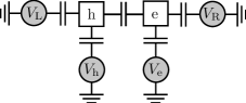
Figure 5: Capacitance network showing the two dots (h and e) connected to the superconducting leads ($V_{\rm L}$ and $V_{\rm R}$) as well as to gate electrodes ($V_{\rm h}$ and $V_{\rm e}$).

As mentioned above, the states $|0_{\scriptscriptstyle\rm h}0_{\scriptscriptstyle\rm e}\rangle$, $|2_{\scriptscriptstyle\rm h}0_{\scriptscriptstyle\rm e}\rangle$, $|0_{\scriptscriptstyle\rm h}2_{\scriptscriptstyle\rm e}\rangle$, and $|2_{\scriptscriptstyle\rm h}2_{\scriptscriptstyle\rm e}\rangle$ represent a two qubit system. In section 3, we have shown that the system left alone relaxes to the state $|0_{\scriptscriptstyle\rm h}0_{\scriptscriptstyle\rm e}\rangle$. This provides an automatic initialization of the qubit. In this section, we outline a possible scheme for the qubit manipulation by irradiation pulses. It is important to note that the manipulation is all-electric, achievable by modulating the gate voltages. Figure 5 depicts the system of the two dots together with four gates. Two of them, $V_{\rm L}$ and $V_{\rm R}$, address the superconducting leads and the remaining two, $V_{\rm h}$ and $V_{\rm e}$, are the back gates for the dots in the superconducting wire already used above to tune the dots.

Since all the energy differences between the qubit states are nondegenerate, a specific transition can be addressed by tuning the irradiation frequency $\omega$ to the energy difference between the states involved. To understand the details of the manipulation, it is important to note that the voltages not only shift the positions of the levels $\varepsilon_{\rm h,e}$ with respect to corresponding electrodes, they also produce time-shifts in the superconducting phases of the electrodes, so that $\tilde{\Delta}_{\rm e}\to\tilde{\Delta}_{\rm e}e^{i\phi_{\rm R}(t)}$ with $\dot{\phi}_{\rm R}=2eV_{\rm R}(t)/\hbar$, and similar for $\tilde{\Delta}_{\rm h}$. Neglecting this would lead to the confusing and incorrect conclusion that transitions can be induced even without capacitances between the dots and the gate electrodes. In fact, the division of the a.c. voltage in a capacitative network is crucial for the transitions to occur.

To make this explicit, it is constructive to perform a unitary (gauge) transformation that cancels the time dependence of $\tilde{\Delta}_{\rm h,e}$. After this, the only effect of the a.c. voltage is the modulation of the levels given by

$$\delta\varepsilon_{\rm h}/e=a_{\rm hh}(V_{\rm h}-V_{\rm L})+a_{\rm he}(V_{\rm e}-V_{\rm L})+a_{\rm h}(V_{\rm R}-V_{\rm L}),$$ (7)

$$\delta\varepsilon_{\rm e}/e=a_{\rm ee}(V_{\rm e}-V_{\rm R})+a_{\rm eh}(V_{\rm h}-V_{\rm R})+a_{\rm e}(V_{\rm L}-V_{\rm R});$$ (8)

where the coefficients $a$, $|a|<1$, are obtained from the voltage division in the capacitance network. In zeroth order in $|\tilde{\Delta}|/\hbar\omega$, the irradiation pulses do not induce transitions between the qubit states but rather change their mutual energy differences. Transitions appear in first order with a corresponding non-diagonal matrix element of the order of $|\tilde{\Delta}\,\delta\varepsilon|/\hbar\omega$.

As a concrete example, let us tune $\hbar\omega$ to the energy difference between the states $|2_{\scriptscriptstyle\rm h}0_{\scriptscriptstyle\rm e}\rangle$ and $|2_{\scriptscriptstyle\rm h}2_{\scriptscriptstyle\rm e}\rangle$. The Hamiltonian $H^{\prime\prime}$ in the relevant subspace spanned by these two states reads

$$H^{\prime\prime}=\left(\begin{array}[]{cc}0&\tilde{\Delta}_{\rm e}^{*}\\ \tilde{\Delta}_{\rm e}&\hbar\omega+2\,\delta\varepsilon_{\rm e}(t)\end{array}\right)$$ (9)

where the energies are measured with respect to the reference state $|2_{\scriptscriptstyle\rm h}0_{\scriptscriptstyle\rm e}\rangle$. A constant resonant irradiation modulating $\delta\varepsilon_{e}(t)$ harmonically with amplitude $\bar{\varepsilon}$ results in Rabi oscillations between these states at a frequency $\omega_{\rm R}=|\tilde{\Delta}_{\rm e}|J_{1}(2\bar{\varepsilon}/\hbar\omega)/\hbar$, where $J_{1}(x)$ denotes a Bessel function of the first kind. If one applies the irradiation for a time $t_{\pi}=\pi/\omega_{\rm R}$, corresponding to a $\pi$ pulse, the effect is a c-NOT gate: Depending on the state $|0_{\scriptscriptstyle\rm h}\rangle$ or $|2_{\scriptscriptstyle\rm h}\rangle$ of the hole qubit, the state of the electron qubit is inverted or not. Note that the c-NOT gate is a fundamental two qubit gate which together with arbitrary single qubit operations can simulate any quantum circuit [23].

The readout of the two-qubit gate occurs via the radiative decay of the state $|2_{\scriptscriptstyle\rm h}2_{\scriptscriptstyle\rm e}\rangle$ which is the only one with a sizable radiative decay rate. The fact that one can read only the probability of this state is known to present no principal obstacle for measuring more complicated variables, since one can perform an arbitrary unitary operation in the Hilbert space before the read-out. In fact, full tomography of a two qubit density matrix has been demonstrated recently by resorting only to the measurement of a single fixed operator [26]. We remark that the main source of decoherence in the qubits is due to voltage fluctuations in the environment.

6 Photon-spin entanglement

The state $\Psi_{1}$, after the emission of the first photon, exhibits entanglement between the photon and the dot degrees of freedom. This state is however not stable and will decay further as explained above. Applying a large pulse on $\varepsilon_{\rm e}$ with $\delta\varepsilon_{\rm e}\gg|\Delta_{\rm e}|$ which shifts all the levels of the electron dot levels above the superconducting gap $|\Delta_{\rm e}|$ and thereby empties the electron side of the double dot, we arrive at the state

$$\Psi_{\rm ent}\propto|{\downarrow}_{\scriptscriptstyle\rm h}\rangle|+\rangle+|{\uparrow}_{\scriptscriptstyle\rm h}\rangle|-\rangle,$$ (10)

where the spin degree of the last remaining hole is entangled with the photon polarization; note that alternatively, one could empty the hole side of the dot to obtain a single electron whose spin is entangled with the photon polarization. A drawback of this procedure arises from the fact that the pulse which empties the dot has to be applied after the first photon has been emitted and before the second emission takes place. However, the process is stochastic and measurement is not an option as it would destroy entanglement. Therefore, the best we can do is to optimize the time at which we apply the pulse such as to maximize the probability that one photon is emitted. We note that the probabilities $P_{n}(t)$ that $n$-photons have been emitted at time $t$ to follow the rate equations

$$\dot{P}_{0} = -\Gamma_{\rm ph}P_{0}$$ (11)

$$\dot{P}_{1} = \Gamma_{\rm ph}(P_{0}-P_{1})$$ (12)

$$\dot{P}_{2} = \Gamma_{\rm ph}P_{1},$$ (13)

with the solution $P_{0}=\exp(-\Gamma_{\rm ph}t)$, $P_{1}=\Gamma_{\rm ph}t\exp(-\Gamma_{\rm ph}t)$, and $P_{2}=1-P_{0}-P_{1}$. The probability $P_{1}$ for a single photon is maximized at a time $t_{\rm opt}=\Gamma_{\rm ph}^{-1}$ with the maximal probability $P_{1}(t_{\rm opt})=1/e\approx 0.37$ to have a single photon emitted. Conditioning the experiment on the fact that there is at least a photon emitted, offers a way to increase the success probability $P_{\rm succ}$ to a value $P_{\rm succ}=P_{1}/(P_{1}+P_{2})=1/(e-1)\approx 0.58$ for the optimal time $t_{\rm opt}$. In fact, the conditional success probability $P_{\rm succ}$ approaches one for short times $t$, i.e, when the kick-out pulse is applied immediately after the biexciton state has been prepared. However, the large success probability comes with the expense that the probability $P_{1}+P_{2}$ to obtain a photon at all becomes vanishingly small.

7 Spin measurement

Figure 6: The measurement of the spin of a single hole is done via its conversion into the polarization of a photon. The figure shows the possible initial configurations of the hole spin and the production of the photon. The latter requires mixing due to a superconducting lead.

In the situation where we the dots are in state $|1_{\scriptscriptstyle\rm h}0_{\scriptscriptstyle\rm e}\rangle$, we might be interested to find out whether the single hole is in the spin up or down state. For example, in the previous section we have discussed a possible way to generate entanglement between the hole spin and the polarization of an emitted photon. In this case, we need to be able to measure the spin degree of freedom in order to test the entanglement. We propose a way to transfer the spin state onto the polarization of a photon which can then be easily probed using a polarizer and a photon counter; note that this procedure has to be applied fast compared to $\tilde{\Gamma}_{\rm ph}$ as the secondary photon processes offer a way to recombine the hole via the creation of a quasiparticle in the lead. Imagine that the dot is in the state $|{\uparrow}_{\scriptscriptstyle\rm h}0_{\scriptscriptstyle\rm e}\rangle$. By tuning the pair of states $|1_{\scriptscriptstyle\rm h}0_{\scriptscriptstyle\rm e}\rangle,|1_{\scriptscriptstyle\rm h}2_{\scriptscriptstyle\rm e}\rangle$ into degeneracy (by choosing $\varepsilon_{\rm e}=-U_{\rm e}-U_{\rm he}$), we start mixing them into each other with amplitude $\tilde{\Delta}_{\rm e}$, cf. figure 2. Starting with the state $|{\uparrow}_{\scriptscriptstyle\rm h}0_{\scriptscriptstyle\rm e}\rangle$, we coherently evolve into the state $|{\uparrow}_{\scriptscriptstyle\rm h}2_{\scriptscriptstyle\rm e}\rangle$. Subsequently, a photon with $+$ polarization can be created and the dot ends up in the state $|0_{\scriptscriptstyle\rm h}{\downarrow}_{\scriptscriptstyle\rm e}\rangle$ where it remains until a secondary photon process occurs. It is easy to see that if the dot is initially in the $|{\downarrow}_{\scriptscriptstyle\rm h}0_{\scriptscriptstyle\rm e}\rangle$ state the photon produced will carry the $-$ polarization. Therefore, we have obtained the situation where the spin of the hole is transferred into the polarization of a photon thereby providing a way to measure the spin of the hole. The same procedure can also be applied to measure the spin of a single electron if one brings the states $|0_{\scriptscriptstyle\rm h}1_{\scriptscriptstyle\rm e}\rangle$ and $|2_{\scriptscriptstyle\rm h}1_{\scriptscriptstyle\rm e}\rangle$ into degeneracy by choosing $\varepsilon_{\rm h}=-U_{\rm h}-U_{\rm he}$.

8 Summary

We have outlined possibilities to use the Josephson LED as device for quantum information purposes. We have shown the possibility to create entangled photon pairs on-demand. Furthermore, the device emulates a two qubit system for which we have proposed a scheme for preparation, operation, and measurement. We have demonstrated the possibility to entangle the spin of a particle in one of the dots with the polarization of an emitted photon. Additionally, we have shown an alternative way to transfer the spin of the particle into the polarization of a photon which can be used as a method to measure the spin.

References

References

- [1] van Wees B J and Takayanagi H 1997 The superconducting proximity effect in semiconductor-superconductor systems: Ballistic transport, dimensionality and sample specific properties In Mesoscopic Electron Transport, eds. Sohn L L, Schön G and Kouwenhoven L P, volume 345 of NATO ASI Series E (Kluwer Academic Publishers: Dordrecht)
- [2] Doh Y J, van Dam J A, Roest A L, Bakkers E P, Kouwenhoven L P and De Franceschi S 2005 Tunable supercurrent through semiconductor nanowires Science 309 272
- [3] van Dam J A, Nazarov Yu V, Bakkers E P A M, De Franceschi S and Kouwenhoven L P 2006 Supercurrent reversal in quantum dots Nature 442 667
- [4] Xiang J, Vidan A, Tinkham M, Westervelt R M and Lieber C M 2006 Ge/Si nanowire mesoscopic Josephson junctions Nature Nanotechnology 1 208
- [5] Recher P, Nazarov Yu V and Kouwenhoven L P 2009 The Josephson light-emitting diode arXiv:0902.4468
- [6] Michler P, Imamoğlu A, Mason M D, Carson P J, Strouse G F and Buratto S K 2000 Quantum correlation among photons from a single quantum dot at room temperature Nature 406 968
- [7] Zwiller V, Blom H, Jonsson P, Panev N, Jeppesen S, Tsegaye T, Goobar E, Pistol M E, Samuelson L and Björk G 2001 Single quantum dots emit single photons at a time: Antibunching experiments Appl. Phys. Lett. 78 2476
- [8] Santori C, Fattal D, Vučković J, Solomon G S and Yamamoto Y 2002 Indistinguishable photons from a single-photon device Nature 419 594
- [9] Zrenner A, Beham E, Stufler S, Findeis F, Bichler M and Abstreiter G 2002 Coherent properties of a two-level system based on a quantum-dot photodiode Nature 418 612
- [10] Li X, Wu Y, Steel D, Gammon D, Stievater T H, Katzer D S, Park D, Piermarocchi C and Sham L J 2003 An all-optical quantum gate in a semiconductor quantum dot Science 301 809
- [11] Warburton R J, Schäflein C, Haft D, Bickel F, Lorke A, Karrai K, Garcia J M, Schoenfeld W and Petroff P M 2000 Optical emission from a charge-tunable quantum ring Nature 405 926
- [12] Atatüre M, Dreiser J, Badolato A, Högele A, Karrai K and Imamoğlu A 2006 Quantum-dot spin-state preparation with near-unity fidelity Science 312 551
- [13] Atatüre M, Dreiser J, Badolato A and Imamoğlu A 2007 Observation of Faraday rotation from a single confined spin Nature Phys. 3 101
- [14] Gerardot B D, Brunner D, Dalgarno P A, Öhberg P, Seidl S, Kroner M, Karrai K, Stoltz N G, Petroff P M and Warburton R J 2008 Optical pumping of a single hole spin in a quantum dot Nature 451 441
- [15] Brunner D, Gerardot B D, Dalgarno P A, Wüst G, Karrai K, Stoltz N G, Petroff P M and Warburton R J 2009 A coherent single-hole spin in a semiconductor Science 325 70
- [16] Khaetskii A V and Nazarov Yu V 2000 Spin relaxation in semiconductor quantum dots Phys. Rev. B 61 12639
- [17] Moreau E, Robert I, Manin L, Thierry-Mieg V, Gérard J M and Abram I 2001 Quantum cascade of photons in semiconductor quantum dots Phys. Rev. Lett. 87 183601
- [18] Benson O, Santori C, Pelton M and Yamamoto Y 2000 Regulated and entangled photons from a single quantum dot Phys. Rev. Lett. 84 2513
- [19] Gywat O, Burkard G and Loss D 2002 Biexcitons in coupled quantum dots as a source of entangled photons Phys. Rev. B 65 205329
- [20] Santori C, Fattal D, Pelton M, Solomon G S and Yamamoto Y 2002 Polarization-correlated photon pairs from a single quantum dot Phys. Rev. B 66 045308
- [21] Stevenson R M, Young R J, Atkinson P, Cooper K, Ritchie D A and Shields A J 2006 A semiconductor source of triggered entangled photon pairs Nature 439 179
- [22] Akopian N, Lindner N H, Poem E, Berlatzky Y, Avron J, Gershoni D, Gerardot B D and Petroff P M 2006 Entangled photon pairs from semiconductor quantum dots Phys. Rev. Lett. 96
- [23] Nielsen M A and Chuang I L 2000 Quantum Computation and Quantum Information (Cambridge University Press: Cambridge)
- [24] Lloyd S 1996 Universal quantum simulators Science 273 1073
- [25] Weisbuch C and Vinter B 1991 Quantum Semiconductor Structures: Fundamentals and Applications (Academic Press: San Diego)
- [26] DiCarlo L, Chow J M, Gambetta J M, Bishop L S, Johnson B R, Schuster D I, Majer J, Blais A, Frunzio L, Girvin S M and Schoelkopf R J 2009 Demonstration of two-qubit algorithms with a superconducting quantum processor Nature 460 240