Cosmic ray positron excess:
is the dark matter solution a good bet?

Abstract

The recent observation by the PAMELA satellite of a rising positron fraction up to $\sim$ 100 GeV has triggered a considerable amount of putative interpretations in terms of dark matter (DM) annihilation or decay. Here, we make a critical reassessment of such a possibility, recalling the elementary conditions with respect to the standard astrophysical background that would make it likely, showing that they are not fulfilled. Likewise, we argue that, as now well accepted, DM would need somewhat contrived properties to contribute significantly to the observed positron signal, even when including e.g. clumpiness effects. This means that most of natural DM candidates arising in particle physics beyond the standard model are not expected to be observed in the cosmic antimatter spectrum, unfortunately. However, this does not prevent them from remaining excellent DM candidates, this only points towards the crucial need of developing much more complex detection strategies (multimessenger, multiwavelength, multiscale searches).

1 Introduction

Since its discovery in the early 1930’s by Zwicky (1933), the DM issue has remained unsolved. There are basically two different theoretical ways to address this issue, one considering a new additional component of exotic matter in the form of weakly interacting massive particles (WIMPs), the other involving modifications of general relativity (sometimes even both). Both have relevant motivations, the former from particle physics beyond the standard model (see e.g. Jungman et al., 1996; Murayama, 2007, for reviews) and structure formation (see a more detailed discussion in e.g. Peebles, 2009), the latter from more empirical attempts at the galaxy scale (Milgrom, 1983) or more recently in the context of extra-dimensional theories (e.g. Dvali et al., 2000). One of the appealing flavor of the former hypothesis, that we will consider in the following, is the possibility to test it with a broad variety of existing or coming experimental devices. Among interesting astroparticle signatures, gamma rays and antimatter CRs have long been considered as promising DM tracers (Gunn et al., 1978; Silk and Srednicki, 1984), but it is only recently that precision data have become available to look for non-standard features (Carr et al., 2006; Salati, 2007).

Although the rise in the local cosmic positron fraction at the GeV energy scale has been observed for a long time (e.g. Fanselow et al., 1969; Barwick et al., 1997; Alcaraz et al., 2000), the statistics recently released by the PAMELA collaboration (Adriani et al., 2009) is unprecedented and covers a much larger energy range, up to 100 GeV. The secondary origin of these positrons seems unlikely (Moskalenko and Strong, 1998; Delahaye et al., 2009a), even if theoretical uncertainties are still large. The main questions are therefore (i) whether or not standard astrophysical sources may supply for such a signal and (ii) whether or not DM annihilation or decay is expected to be also observed in this channel. It is noteworthy that this was already discussed by Boulares (1989) twenty years ago, where the author pointed out that a pulsar origin was the best explanation to a rising positron fraction. It is not less interesting and sociologically striking to take a census of the articles addressing point (i) versus those focused on point (ii). Anyway, in this proceeding, we aim at discussing this issue concentrating on the local cosmic positron signal only, forgetting about other counterparts. We will first review the astrophysical backgrounds of secondary and primary origins; then, we will check whether DM could naturally yield prominent imprints in the cosmic positron spectrum, before concluding.

2 Astrophysical backgrounds

2.1 Bases of CR propagation

The global understanding of Galactic CRs at the GeV-TeV scale is rather well established. CRs are accelerated by shock waves at the vicinity of violent events like supernova (SN) explosions, and further diffuse erratically in the interstellar medium (ISM) by bouncing on moving magnetic turbulences. This diffusive motion is accompanied by other processes whose respective impacts depend on the cosmic ray species: convection that drives CRs away from the Galactic plane (negligible above a few GeV), energy losses (affecting mostly leptons), diffusive reacceleration (negligible above a few GeV), spallation reactions with the ISM gas (for nuclei only). The general formalism of CR transport was designed a long time ago in the seminal book of Ginzburg and Syrovatskii (1964), and refined many times since then (see e.g. Berezinskii et al., 1990; Strong et al., 2007). The master equation that describes the CR transport in phase-space looks like a classical current conservation equation:

$$\widehat{\cal D}_{\mu}\,\widehat{\cal J}^{\mu}+\widehat{\cal D}_{E}\,\widehat{\cal J}^{E}=\widehat{\cal Q}\;.$$ (1)

Given a CR differential number density ${\cal N}=dn/dE$, the spacetime-like current is reminiscent from the Fick law and the heat equation, $\widehat{\cal J}^{\mu}=({\cal N},\left\{\vec{\nabla}K_{d}(E)-\vec{V}_{c}\right\}{\cal N})$, for which the associated transport operator reads $\widehat{\cal D}_{\mu}=(\partial_{t}+\Gamma_{\rm spal}+\Gamma_{\rm dec},-\vec{\nabla})$. The energy component is merely $\widehat{\cal J}^{E}={\cal N}$, on which acts $\widehat{\cal D}_{E}=\partial_{E}(dE/dt+K_{E}\partial_{E})$. Appearing above, $\widehat{\cal Q}$ is the source term, $K_{d}$ the spatial diffusion coefficient, $K_{E}$ the reacceleration coefficient, $\Gamma_{\rm spal/dec}$ the spallation/decay rate, $\vec{V}_{c}$ the convection velocity, and $dE/dt$ the energy loss term. Each of these ingredients is by itself subject of intense researches, so that many simplifying assumptions are usually made in phenomenological analyses. In general, one assumes that spatial diffusion proceeds isotropically and that the diffusion coefficient is homogeneous in the diffusion zone, only scaling with the CR rigidity $\propto{\cal R}^{\delta}$. Apart from the energy losses and the spallation or decay rate which can be predicted independently, the propagation parameters are usually constrained with measurements of CR nuclei, more precisely with secondary to primary ratios like B/C (see e.g. Strong and Moskalenko, 1998; Maurin et al., 2001). Important features of such a modeling are the spatial extent of the diffusion zone (usually taken as a cylindrical slab) and the diffusion coefficient, and we stress that the related uncertainties are still rather large (Maurin et al., 2001). In the following, we will adopt a thick cylindrical diffusion zone of radius $R=20$ kpc and half-width $L=4$ kpc, unless specified otherwise.

In some cases, analytical solutions to the diffusion equation can be found in terms of Green functions $\cal{G}$, which obey $\widehat{\cal D}_{\mu,E}\,{\cal G}^{\mu,E}(\widehat{x}\leftarrow\widehat{x}_{s})=\delta^{3}(\vec{x}_{s}-\vec{x})\delta(t_{s}-t)\delta(E_{s}-E)$. For instance, assuming both steady state, which is relevant for a constant CR injection rate, and an infinite 3D diffusion space, thereby neglecting the spatial boundary conditions, the propagators for protons (or antiprotons) and electrons (or positrons) are simply given by:

$${\cal G}_{p}(\vec{x}\leftarrow\vec{x}_{s})=\frac{1}{4\pi K(E)||\vec{x}-\vec{x}_{s}||}\;,\;\;\;{\cal G}_{e}(E,\vec{x}\leftarrow E_{s},\vec{x}_{s})=\frac{1}{b(E)\left\{\pi\lambda^{2}\right\}^{3/2}}\,\exp\left\{-\frac{|\vec{x}-\vec{x}_{s}|^{2}}{\lambda^{2}}\right\}\;.$$ (2)

Only spatial diffusion has been considered for protons (no energy losses, convection, nor spallation — fair approximation above a few GeV). For electrons, the mixed impact of (local) energy losses $dE/dt=-b(E)$ and of diffusion is encoded in the propagation scale

$$\lambda(E,E_{s})=\left\{4\int_{E}^{E_{s}}dE^{\prime}\,K_{d}(E^{\prime})/b(E^{\prime})\right\}^{1/2}\;,$$ (3)

and other processes are neglected. This illustrates that while proton and electron transport is described by the same equation, these species can actually diffuse quite differently because of the relative differences in the processes they experience. For electrons in the GeV-TeV range, energy losses are dominated by inverse Compton (IC) scattering on the interstellar radiation field (ISRF) including the cosmic microwave background (CMB), and by synchrotron losses on the Galactic magnetic field. In the local environment, the typical energy loss timescale at $E_{0}=1$ GeV is $\tau\simeq 315$ Myr. With a typical diffusion coefficient of $K_{0}\simeq 0.01\,{\rm kpc^{2}/Myr}$, one finds $\lambda\sim 3.5$ kpc, which justifies a posteriori the use of the local ISRF and magnetic field to compute the energy losses (Delahaye et al., 2009a). In the Thomson approximation, $b(E)=(E_{0}/\tau)\left\{\epsilon\equiv E/E_{0}\right\}^{2}$ (Blumenthal and Gould, 1970), which implies that the propagation scale strongly decreases with energy.

The previous Green functions reveal an important difference between stable nuclei and electrons: the former have a long range propagation scale (above a few GeV) only limited by the finite spatial extent of the diffusion zone, while the latter have a short range propagation scale limited by energy losses. Therefore, spatial fluctuations of the CR injection rate will be less important for stable nuclei (except below a few GeV, when spallation and convection become important) than for electrons. This implies a more local origin of high energy CR electrons and positrons, and means that time fluctuations in their local injection rate induces strong local effects.

2.2 Astrophysical positrons

Positrons of astrophysical origin can be secondaries or primaries. Secondaries are produced from spallation reactions of CR nuclei (mostly protons and $\alpha$) with the ISM gas (H and He). Primaries can be directly produced in the intense magnetic field hosted by sources like pulsars (Ostriker and Gunn, 1969) and further accelerated in the surrounding shocked medium, or could also be secondaries created from spallation processes within acceleration sites like supernova remnants (SNRs) (Blasi, 2009). Thus, the secondary positron source term depends on the spatial distribution of CR nuclei and of the ISM gas:

$${\cal Q}_{s}(E,\vec{x})=4\pi\sum_{i,j}\int dE^{\prime}\,\phi_{i}(E^{\prime},\vec{x})\,\frac{d\sigma_{ij}(E^{\prime},E)}{dE}\,n_{j}(\vec{x})\;,$$ (4)

where $i$ flags the CR species of flux $\phi$ and $j$ the ISM gas species of density $n$, the latter being concentrated within the thin Galactic disk. $d\sigma_{ij}(E^{\prime},E)$ is the inclusive cross section for a CR-atom interaction to produce a positron of energy $E$. This differential cross section $\approx\theta(E^{\prime}-E)\theta(E^{\prime}-E_{\rm th})\sigma_{ij}/E$ with $E_{\rm th}\sim 5$ GeV (Delahaye et al., 2009a), so that if $\phi$ is described by a power law $\phi_{0}\epsilon^{-\gamma_{s}}$, then ${\cal Q}_{s}^{i,j}(E,\vec{x})\approx 4\pi\phi_{i}(E,\vec{x})\,\sigma_{ij}n_{j}(\vec{x})/(\gamma_{s}-1)$. Moreover, since nuclei have a long range propagation scale and since the ISM gas does not exhibit strong spatial gradient over the kpc scale in the Galactic disk (Ferrière, 2001), one can further approximate $\phi$ and $n$ to their local values to get rough estimates of ${\cal Q}_{s}$. For instance, by considering only the proton-hydrogen interaction, and taking $\phi_{p}(E)=1.3\,{\rm cm^{-2}s^{-1}sr^{-1}((E-m_{p})/1{\rm GeV})^{-2.72}}$ (Donato et al., 2001), $n_{H}=1\,{\rm cm^{-3}}$ and $\sigma_{pp}=10$ mb, we end up with ${\cal Q}_{s}(E)\approx 2\times 10^{-27}\epsilon^{-2.72}{\rm cm^{-3}GeV^{-1}s^{-1}}$, which is actually quite close to the accurate calculation (Delahaye et al., 2009a). Since the positron horizon is limited to a few kpc, the source may be modeled by an injection rate homogeneously distributed in an infinite thin Galactic disk of half-height $h\sim 100$ pc like ${\cal Q}_{s}(E,\vec{x})=2h\delta(z)\,Q_{0s}\epsilon^{-\gamma_{s}}$. This allows to infer the local flux inside that disk, relevant for an observer on Earth:

$$\phi_{s,\odot}(E)=\frac{\beta c}{4\pi}\int dE_{s}\int d^{3}\vec{x}_{s}\,{\cal G}_{e}(E,\vec{x}_{\odot}\leftarrow E_{s},\vec{x}_{s}){\cal Q}_{s}(E_{s},\vec{x}_{s})=\frac{\beta c\,2h\,Q_{0s}}{2\pi^{3/2}b(E)}\int\frac{dE_{s}}{\lambda}\,\epsilon_{s}^{-\gamma_{s}}\approx\frac{c\,Q_{0s}\,h\,\sqrt{\tau}\,\epsilon^{-\gamma_{s}-\frac{1}{2}(\delta+\alpha-1)}}{2\pi^{3/2}\sqrt{K_{0}}(\gamma_{s}-1)}\,\;.$$ (5)

Here, we have taken a diffusion coefficient $K_{d}(E)=K_{0}\epsilon^{\delta}$ and an energy loss rate $b(E)=(E_{0}/\tau)\,\epsilon^{\alpha}$, where $\alpha=2$ in the Thomson approximation. Using $\delta=0.7$, $\alpha=2$ and the values given above for the other parameters, Eq. (5) gives $\phi_{s,\odot}(E)\approx 8.5\times 10^{-3}\epsilon^{-3.57}{\rm cm^{-2}GeV^{-1}s^{-1}sr^{-1}}$, overshooting the exact calculation by a factor of 2 only (Delahaye et al., 2009a, b).

Eq. (5) makes explicit the influence of the main propagation parameters: the energy loss timescale $\tau$ and the diffusion coefficient normalization $K_{0}$ set the positron flux amplitude, and their energy dependence slightly shapes the spectrum. Since the B/C ratio constrains mostly the ratio $K(E)/L$ (Maurin et al., 2001), where $L$ is the vertical extent of the diffusion zone, it is not surprising that the min (max) model of Donato et al. (2004), which was designed to minimize (maximize) the primary antiproton flux coming from DM annihilation, is actually found to maximize (minimize) the secondary positron flux. Indeed, it is associated with a small value of $L=1$ kpc (15 kpc), which has a corresponding small (large) value of $K_{0}$ to fulfill the B/C constraint. Likewise, the logarithmic slope of the diffusion coefficient $\delta$ is larger in the min setup, leading to a softer spectrum than in the max case. These extreme configurations, all compatible with the B/C constraints, are useful to bracket the theoretical uncertainties.

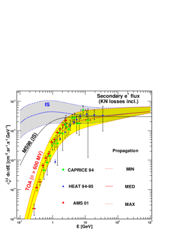
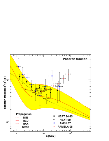
Figure 1: Left: secondary positron flux and theoretical uncertainties. Right: corresponding positron fraction. These plots are adapted from Delahaye et al. (2009b).

In Fig. 1, we plot the latest results obtained by Delahaye et al. (2009b) for the secondary positron flux, where a full relativistic treatment of the energy losses, i.e. beyond the Thomson approximation, was used at variance with the earlier calculations by Moskalenko and Strong (1998) and Delahaye et al. (2009a). The right panel shows the secondary flux at the Earth, where the top of atmosphere (TOA) signal is corrected with a Fisk potential of 600 MV to account for solar modulation, while the right panel is the corresponding positron fraction defined by $f=\phi_{e^{+}}/(\phi_{e^{+}}+\phi_{e^{-}})$. For the fraction, we fitted the electron flux on the AMS data (Aguilar et al., 2002) below 20 GeV, and the full denominator itself on the Fermi data (Abdo et al., 2009) above. Predictions are shown against the data from (Boezio et al., 2000; DuVernois et al., 2001; Aguilar et al., 2002) for the positron flux, and from (Barwick et al., 1997; Beatty et al., 2004; Aguilar et al., 2007) for the positron fraction. For the latter, are also reported the recent results obtained by the PAMELA collaboration (Adriani et al., 2009). We stress that though the theoretical uncertainties are large, of about one order of magnitude in terms of flux, our predictions encompass the data. However, from the spectral trend observed in the positron fraction, it seems unlikely that the excess observed by PAMELA is of secondary origin. This naturally leads to the question of whether or not standard astrophysical sources may provide enough primary positrons to explain this fraction rise, which, from Fig. 1, should amount up to $\sim 5-10$ times the secondary flux around 100 GeV ($\phi_{s}(100\,{\rm GeV})\simeq 4\times 10^{-10}{\rm cm^{-2}GeV^{-1}s^{-1}sr^{-1}}$).

For primary electrons and positrons, the approximations made above hold, except that the source term will differ. Assuming again that standard sources (SNRs and pulsars) are homogeneously distributed in a thin disk of volume $V_{d}=2\pi\,h\,R^{2}$, the injection of CR can be written as follows: ${\cal Q}_{p}(E,\vec{x})\approx 2\,h\delta(z)\,{\cal Q}_{0p}\epsilon^{-\gamma_{p}}e^{-E/E_{c}}\;,$ where we have introduced an energy cut-off $E_{c}$, and where the normalization ${\cal Q}_{0p}$, which carries the dimensions, can be fixed from energetics, e.g. by requiring that the total rate of injected energy is set by the supernova (SN) explosion rate times the energy input associated with pulsars or SNRs. For SNRs, we can impose that ${\cal Q}_{0p}=\Gamma_{sn}(f\,E_{sn})/\{V_{d}\int dE\,E\,\epsilon^{-\gamma_{p}}e^{-E/E_{c}}\}$, where $\Gamma_{sn}$ is the SN explosion rate in the Galaxy and $E_{sn}$ is the explosion kinetic energy of a single object whose a fraction of $f$ is transferred to electrons; for pulsars, we would use instead ${\cal E}_{0}$, the magnetic energy of which a fraction $f$ would be converted into electron-positron pairs. Thus, the flux of primary electrons and positrons can also be approximated with Eq. (5), replacing for the normalization and keeping in mind that the spectral index $\gamma_{p}$ is different, which again turns out to be a fair approximation (Delahaye et al., 2009b). The ratio of primaries to secondaries, given by $R(E)=\phi_{p,\odot}(E)/\phi_{s,\odot}(E)\approx({\cal Q}_{0p}/{\cal Q}_{0p})\,\epsilon^{-\gamma_{p}+\gamma_{s}}$ allows to perform a quick estimate of the pulsar contribution. With reasonable values $(\gamma_{p},f\,{\cal E}_{0},\Gamma)=(2.2,10^{47}{\rm erg},5/{\rm cy})$, we have $R(100\,{\rm GeV})\gtrsim 1$, which is sufficient to explain the positron fraction data. Anyway, even when treated more accurately such a modeling suffers much larger theoretical uncertainties than secondaries. First, the fraction of accelerated leptons and the averaged injected spectrum are not yet very well constrained by dynamical studies of sources, while important numerical efforts have been undertaken on this topic for a few years (e.g. Ellison et al., 2007). Second and more dramatic, since the explosion rate of supernovæ is only of a few per century in the whole Galaxy, the time and related spatial fluctuations become sizable locally and makes it difficult to justify a smooth injection rate, at least at the kpc scale around an observer. This is particularly relevant for the high energy component of the spectrum for which the typical propagation scale is short, and of which local sources are therefore expected to provide the main part. This is actually well known for decades (Shen, 1970), and was well illustrated by e.g. Kobayashi et al. (2004) for electrons. An important consequence of these local fluctuations is that features in the local spectra of CR electrons and positrons are expected. Anyway, despite the very large uncertainties, local pulsars, which are observed in number in the solar vicinity and whose properties can be constrained, can inject an amount of positrons that is sufficient to explain a rising positron fraction. This was recently nicely discussed in Malyshev et al. (2009). A more detailed study of primary electrons and positrons including local sources will be found in Delahaye et al. (2009b), where it is shown that all current observations can be rather well reproduced with reasonable parameters.

To conclude this part, we stress that the background to consider when looking for exotic signatures in the positron (or electron) spectrum is not only made of secondaries, but also of astrophysical primaries. Moreover, despite the large theoretical uncertainties affecting current predictions, standard sources seem capable to yield the necessary amount of positrons that may explain the positron fraction fairly naturally, without any over-tuning of the parameters. Likewise, we emphasize that the time and spatial fluctuations of the local injection rate — local sources — can lead to a broad diversity of features in the measured spectrum (Delahaye et al., 2009b), which makes it difficult to disentangle different primary components. Finally, it seems now clear that we are far from a standard model of Galactic CRs, especially in the lepton channel, and many issues remain to be addressed in the future, from the CR source description to a more refined propagation modeling.

3 Dark matter and positrons

Positrons were long thought to be good tracers of DM annihilation precisely because they were expected to be of secondary origin only, i.e. with a low level and predictable astrophysical background. As argued in the previous section, this statement is likely not valid anymore. Anyway, to keep the reasoning as general as possible, let us recall some basic conditions for a cosmic messenger to be a good tracer for any exotic signal: (i) the background is not too high with respect to the expected signal, given an experimental sensitivity; (ii) the background is known or predictable, and controled; (iii) specific spectral features in the signal make it unambiguously distinguishable from the background. We did not yet discuss condition (i), but it is clear from the previous section that conditions (ii) and (iii) cannot be fulfilled. From this simple argument, we can hardly hope, at least with current data, to identify a clean DM signature in the local positron spectrum. Nevertheless, it is still well-grounded to ask whether DM is about to provide a sizable signal, should it be mixed with other components. If so, there might still be some hopes for isolating it with future experiments, provided the astrophysical background is being much better understood in the meantime.

We will first review the predictions that can be derived in general cases when modeling the Galactic DM halo with a smooth distribution. Then, we will discuss the potential impact of DM substructures on the expected signal. We will focus our discussion on annihilating DM, disregarding decaying candidates.

3.1 The smooth approximation

Structure formation in a $\Lambda$CDM universe involves non-linear processes as soon as the linear growth of perturbations triggers the gravitational collapse of objects. In this theoretical framework, galaxies are expected to have formed around redshift $z\sim 6$, and have consequently left the linear regime for a long time, so that only numerical experiments can provide detailed information on the DM distribution in those objects. The advent of high resolution numerical simulations in the study of structure formation has led to major breakthroughs during the last two decades, providing a fairly good understanding of the properties of the large scale structures that are observed in current surveys. There are still some important mismatches at the Galactic scale, but this might be due to the important impact of baryons which have not been included to those simulation until recently (see e.g. Primack, 2009, for a discussion on the small scale issues). Anyway, disregarding the potentially large effect induced by baryons, it seems that DM structures at the galactic scale are predicted to have similar smooth DM density distributions, almost spherical and scale-independent. Such a generic density profile was named NFW after their authors Navarro, Frenk and White (Navarro et al., 1997), and is typified by the following function:

$$\rho(r)=\rho_{s}\frac{(r_{s}/r)}{(1+r/r_{s})^{2}}\;,$$ (6)

where $r_{s}$ is a scale radius beyond which the logarithmic slope goes from -1 to -3; $\rho_{s}$ is the scale density. It is noteworthy that more recent results give quite similar smooth DM components scaling like $\rho\sim(r/r_{s})^{-\gamma}$ in the central regions, with $\gamma\approx 1$, though the lack of resolution prevents from making clear predictions at the very center (see e.g. Springel et al., 2008; Diemand et al., 2008). Using such a density shape, derived from theoretical constraints, to describe our Galaxy needs to account for additional observational constraints from stellar kinematics. Basically, although the baryon modeling comes into play with uncertainties, a local density of $\rho_{\odot}(R_{\odot}=8\,{\rm kpc})\sim 0.3\,{\rm GeV.cm^{-3}}$ associated with a scale radius of $r_{s}\lesssim 20$ kpc are fairly compatible with current data (e.g. Klypin et al., 2002; Sofue, 2009; Catena and Ullio, 2009). Now, since the injection rate of the DM annihilation products is $\propto\rho^{2}$, the precise values of the logarithmic slope may have a strong impact on predictions, especially for annihilation close the Galactic center (GC). This is particularly true for $\gamma$-ray flux predictions (Bergström et al., 1998), but not really for CR positrons in the GeV-TeV energy range, since, as discussed above, they cannot pervade beyond a few kpc — for longer range antiprotons, the signal coming from there is anyway diluted by diffusion. Uncertainties in the flux amplitude will be therefore mostly set by those on the local DM environment.

To summarize, let us write the source term associated with DM annihilation:

$${\cal Q}_{\chi}(\vec{x},E) = {\cal S}\,\left\{\frac{\rho(r)}{\rho_{\odot}}\right\}^{2}\,\frac{dN(E)}{dE}\;\;\;{\rm with}\;\;\;{\cal S}\equiv\delta\frac{\mbox{$\langle\sigma v\rangle$}}{2}\left\{\frac{\rho_{\odot}}{\mbox{$m_{\chi}$}}\right\}^{2}\;,$$ (7)

where $\delta=1/2$ (1) for Dirac (Majorana) fermionic WIMPs, and 1 for scalar WIMPs; $\langle\sigma v\rangle$ is the WIMP annihilation cross section, $m_{\chi}$ the WIMP mass and $dN(E)$ the number of CR positrons injected in the energy range $dE$. The different WIMP candidates should have similar annihilation cross sections of $\mbox{$\langle\sigma v\rangle$}\sim 3\times 10^{-26}{\rm cm^{3}/s}$ if they decouple thermally from the primordial bath as a consequence of expansion in the early universe, such a value being fixed by the present cosmological DM density (the generic method to compute the relic abundance can be found in Edsjö and Gondolo, 1997). The local positron spectral shape will primarily depend on the annihilation final states. Three typical final states may basically typify the main features of the positron injection spectra associated with DM annihilation or decay, (i) quarks, say $b\bar{b}$, (ii) $W^{+}W^{-}$ and (iii) $l^{+}l^{-}$ with any charged lepton, say $e^{+}e^{-}$. The spectrum is getting harder and harder from (i) to (iii).

To check whether usual WIMP candidates are about to give a sizable positron flux, it turns out useful to derive the flux in the asymptotic limit of very short propagation scale, which is a rough approximation valid at high energy. The corresponding propagator is therefore ${\cal G}_{e}(E,\vec{x}\leftarrow E_{s},\vec{x}_{s})\xrightarrow{\lambda\rightarrow 0}\delta(E_{s}-E)\delta^{3}(\vec{x}_{s}-\vec{x})/b(E)$ — which only differs from the diffusionless limit by the term $\delta(E_{s}-E)$ that ensures $\lambda\rightarrow 0$ here. If we further assume a direct annihilation in $e^{+}e^{-}$, so that $dN(E)/dE=\delta(E-\mbox{$m_{\chi}$})$, then the asymptotic and exact flux limit reads:

$$\phi^{\chi}_{\odot}(E\rightarrow\mbox{$m_{\chi}$}) \xrightarrow{\chi\chi\rightarrow e^{+}e^{-}} \frac{c}{4\pi}\,\frac{{\cal Q}_{\chi}(\vec{x}_{\odot},E)}{b(E)}=\frac{c}{4\pi}\,\frac{\cal S}{b(E)}$$ (8)

$$\approx 3.2\times 10^{-10}{\rm cm^{-2}GeV^{-1}s^{-1}sr^{-1}}\times$$

$$\frac{\mbox{$\langle\sigma v\rangle$}}{3\times 10^{-26}{\rm cm^{3}/s}}\,\frac{\tau}{10^{16}{\rm s}}\,\left[\frac{\rho_{\odot}}{0.3\,{\rm GeV/cm^{3}}}\right]^{2}\,\left[\frac{\mbox{$m_{\chi}$}}{100\,{\rm GeV}}\right]^{-4}\;.$$

where we have used the Thomson approximation for the energy losses. Note that for $\mbox{$m_{\chi}$}=100$ GeV, this result is pretty close to the prediction of the secondary positron flux at 100 GeV. Since the positron fraction measurement at 100 GeV implies $\sim 5-10$ times more primaries than secondaries, this means that boosting the local DM density by a factor of $\sim 3$ is enough to feed the PAMELA data rather significantly. Nevertheless, this is, at least to our knowledge, the unique example for which one may recover the observed positron fraction at $\sim 100$ GeV without over-tuning the annihilation cross section. Indeed, for other annihilation final states and/or larger WIMP masses, one needs to boost the signal by 2 to 4 orders of magnitude to get enough positrons at 100 GeV to match the measurements (e.g. Baltz and Edsjö, 1998; Cirelli and Strumia, 2008). This is illustrated in the left panel of Fig. 2, where we compare predictions assuming the three annihilation final states discussed above, a smooth NFW density profile and the parameters used in Eq. (8). In this plot, the secondary background is taken from Delahaye et al. (2009a), derived in the Thomson approximation for the energy losses.

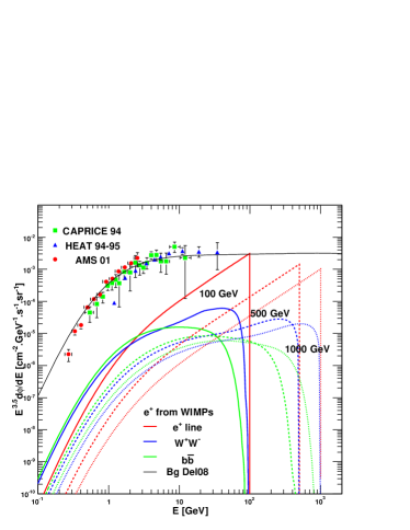
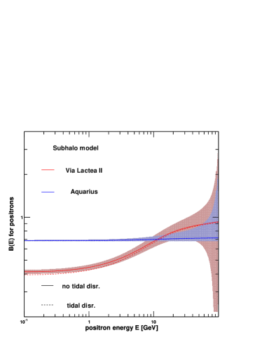
Figure 2: Letf: Predictions of the primary positron fluxes for a smooth NFW DM halo and 3 different annihilation final states, as compared with the secondary background. Right: Boost factors obtained by Pieri et al. (2009) for direct annihilation in $e^{+}e^{-}$ as calculated in the frames of the Via Lactea II (Diemand et al., 2008) and Aquarius (Springel et al., 2008) setups.

To summarize this basic analysis, it seems that few WIMP candidates with thermal relic abundance may provide sufficiently positrons to feed the positron fraction data naturally. Indeed, only those WIMPs with masses around $\sim 100$ GeV and with direct annihilation in $e^{+}e^{-}$ do not need arbitrarily high boost factors with respect to a smooth description of the density profile. Needless to say that there are poor motivations for such models in particle physics beyond the standard model — couplings to heavier leptons would lower the positron yield, however, why 100 GeV particles should couple only to $e^{+}e^{-}$ ? — and that there might already exist limits coming from colliders.Therefore, it is fair to conclude that DM annihilation does not provide a natural explanation to the PAMELA data. However, it is not less fair to ask about the potential impact of DM substructures that are predicted in the frame of $\Lambda$CDM, and that could enhance the local DM density. Note that we have studied the impact of relaxing spherical symmetry for the smooth halo profile in Lavalle et al. (2008a), showing that this has poor effect on predictions.

3.2 Clumpiness effects

DM substructures (called also subhalos or clumps) are predicted in the $\Lambda$CDM paradigm and observed in cosmological N-body simulations. The smallest scales that can grow and further collapse are those encompassed within the WIMP free streaming scale which is set by their intrinsic properties (mass, couplings). For generic WIMPs, the minimal mass scale ranges within $10^{-11}-10^{-3}M_{\odot}$ (Bringmann, 2009). The mass function of these subhalos is usually found close to the $\propto M^{-2}$ prediction of the Press-Schechter theory of self-similar gravitational collapse (Press and Schechter, 1974; Lacey and Cole, 1993) in cosmological N-body simulations (for recent results, see Diemand et al., 2008; Springel et al., 2008). Consequently, without loss of generality, the subhalo distribution in a Milky-Way-like object may be written as (Lavalle et al., 2008):

$$\frac{d\mbox{${n}_{\rm cl}$}(\mbox{${m}_{\rm cl}$},\vec{x})}{d\mbox{${m}_{\rm cl}$}\,dV}=\mbox{${N}_{\rm cl}$}\,\frac{d{\cal P}_{m}(\mbox{${m}_{\rm cl}$},\vec{x})}{d\mbox{${m}_{\rm cl}$}}\,\frac{d\mbox{${\cal P}$}_{v}(\vec{x})}{dV}$$ (9)

where ${N}_{\rm cl}$ is the total number of subhalos, and where $d\mbox{${\cal P}$}_{m}$ and $\mbox{${\cal P}$}_{V}$ denote the mass and spatial probability distribution functions, which are normalized to unity over the whole galaxy extent. ${N}_{\rm cl}$ can be constrained from N-body simulation results, at least in the available resolved mass range — the most recent simulations involving billions of particles can resolve clumps down to $10^{3}-10^{4}\mbox{$M_{\odot}$}$ at the galaxy scale (Diemand et al., 2008; Springel et al., 2008). When extrapolated down to a minimal scale of $10^{-6}\mbox{$M_{\odot}$}$ for subhalos, this number is found in the range $10^{14}-10^{16}$ in a Milky-Way-like galaxy (Lavalle et al., 2008; Pieri et al., 2009). Analytical studies on the tidal disruption of these subhalos in galaxies due to gravitational interactions with the disk or stars show that an important fraction may actually survive (Berezinsky et al., 2008). Besides, although rather spherical, the spatial distribution of subhalos turns out to be different from the smooth DM profile $\rho(r)$ since it exhibits a core radius rather than a cusp in the central parts of N-body galaxies, which is likely due to efficient tidal disruption, and a $r^{-2}$ form rather than $r^{-3}$ in the outskirts. Such a behavior is called antibiased, because $(d\mbox{${\cal P}$}_{V}/dV)/\rho(r)\propto r$ (Diemand et al., 2004), but it is still not clear whether it is still valid for lighter objects, far from being resolved in N-body simulations. Finally, the mass distribution should in principle depend on the location in the galaxy to account for tidal disruption. One can include this effect by calculating the maximal subhalo mass as a function of the galactic radius, keeping constant the normalization of the mass function, which is performed in the full mass range (Pieri et al., 2009). Anyway, as mentioned above, $d\mbox{${\cal P}$}_{m}\propto\mbox{${m}_{\rm cl}$}^{-\alpha}d\mbox{${m}_{\rm cl}$}$ with $\alpha\lesssim 2$.

Since substructures are generically predicted in the $\Lambda$CDM paradigm, and are expected to be impressively numerous in galaxies if DM is made of WIMPs, it is important to include them for consistent calculations of astrophysical signals. Indeed, since the DM annihilation rate is proportional to the squared DM density, the presence of subhalos in the local environment can have strong impact on the antimatter flux (as well as on the diffuse photon emission). We have therefore to derive a method to add the subhalo contribution to the smooth one. Since we have sketched a phase-space distribution of subhalos in Eq. (9), we may think about treating the flux coming from a single object like a stochastic variable, which actually turns out to be correct and powerful (Lavalle et al., 2007, 2008): the typical range of subhalo scale radii, where most of the annihilation proceeds, is indeed smaller than the typical propagation scale, so that clumps can be safely treated as point-like sources. We still further need to specify the properties of a single object, i.e. its mass $m$, position $R$ in the Galaxy, inner density profile and the amount and spectral shape of positrons that it injects. It is conventional to define the subhalo extent by the radius $r_{v}$ at which the average subhalo density is 200 times the critical density $\rho_{c}$ of the universe today. Even when fixing the shape of the inner profile, taking e.g. the NFW model, constraining the associated scale parameters $r_{s}$ and $\rho_{s}$ is in principle much more complicated, since they depend on the formation history. Nevertheless, this history shows up an evolving correlation between the concentration, defined by $c_{v}\equiv r_{v}/r_{s}$, and the subhalo mass — the less massive the more concentrated because formed earlier, in a denser universe. Thus, the knowledge of this concentration function at $z=0$ allows to specify the subhalo parameters entirely. Not only does this concentration function depend on the subhalo mass, but also on the its location in the Galaxy, since more concentrated objects resist more efficiently to tidal effects. It is convenient to define the annihilation volume of a single object: $\xi(m,R)=4\pi\int_{0}^{r_{v}}dr\,r^{2}\,\left\{\frac{\mbox{${\rho}_{\rm cl}$}(m,R,r)}{\rho_{\odot}}\right\}^{2}\;.$ This actually defines the volume needed from a constant density of $\rho_{\odot}$ to produce the actual subhalo injection rate, and somehow measures the ratio of its intrinsic emissivity to the local emissivity. Armed with this definition, it is straightforward to derive the local average flux associated with the whole subhalo population (Lavalle et al., 2007, 2008):

$$\phi^{\chi}_{{\rm cl},\odot}(E) = \frac{\beta c}{4\pi}\,\mbox{${N}_{\rm cl}$}\,{\cal S}\,\langle\langle\xi(\vec{x}_{s})\rangle_{m}\widetilde{\cal G}(\vec{x}_{\odot}\leftarrow\vec{x}_{s})\rangle_{V}\;\;\;{\rm where}\;\;\;\widetilde{\cal G}(\vec{x}_{\odot}\leftarrow\vec{x}_{s})=\int_{E}^{\mbox{$m_{\chi}$}}dE_{s}\,{\cal G}(\vec{x}_{\odot},E\leftarrow\vec{x}_{s},E_{s})\,\frac{dN(E_{s})}{dE_{s}}$$ (10)

$$\xrightarrow{\lambda\rightarrow 0} \frac{\beta c}{4\pi}\,\mbox{${N}_{\rm cl}$}\,{\cal S}\,\langle\xi(\vec{x}_{\odot})\rangle_{m}\,\frac{d\mbox{${\cal P}$}_{V}(\vec{x}_{\odot})}{dV}\,\frac{1}{b(E)}\,\frac{dN(E)}{dE}\;,$$

where $\langle\rangle_{x}$ denotes the average performed with the distribution $\mbox{${\cal P}$}_{x}$, and the latest line is the limit corresponding to a vanishingly small propagation scale $\lambda\rightarrow 0$.

In order to check whether a clumpy DM halo leads to a larger positron flux, it is useful to compute the ratio of both predictions. Of course, clumps are not merely additional mass in the halo, there should be some consistency as well as observational constraints to obey. In fact, the census of subhalos in N-body simulation rests on the mass resolution: since the galactic scale is described quite accurately, one can consider that whatever the discreteness of its content, an N-body galaxy will have a constant mass. Therefore, to model the Galaxy in a consistent manner, a certain fraction of mass should be removed from the smooth DM profile when adding clumps: $\rho(r)\rightarrow(1-f)\rho(r)$, where $f=\mbox{${N}_{\rm cl}$}\langle\mbox{${m}_{\rm cl}$}\rangle_{m}/M_{\rm MW}$. The potential problem with such a procedure is that as soon as the spatial distribution of subhalos differs from the smooth distribution, then the average local DM density is modified (Lavalle et al., 2008), which can lead to comparing situations with different local average DM densities. Anyway, we can now derive the ratio of the flux prediction for the smooth case to that for the clumpy case, so-called boost factor:

$${\cal B}_{\odot}(E)=(1-f)^{2}+\frac{\phi^{\chi}_{{\rm cl},\odot}(E)}{\phi^{\chi}_{\odot}(E)}\xrightarrow{\lambda\rightarrow 0}(1-f)^{2}+\mbox{${N}_{\rm cl}$}\,\frac{d\mbox{${\cal P}$}_{V}(\vec{x}_{\odot})}{dV}\,\langle\xi(\vec{x}_{\odot})\rangle_{m}\;,$$ (11)

where the limit of vanishingly small propagation scale is obtained from Eq. (8) and Eq. (10). This expression is quite natural: the boost limit is only given by the local number density of objects $\mbox{${N}_{\rm cl}$}\,d\mbox{${\cal P}$}_{V}(\vec{x}_{\odot})/dV$ times the average annihilation volume of a single object $\langle\xi(\vec{x}_{\odot})\rangle_{m}$ (which is normalized to the local smooth luminosity by definition, see above). Before taking a numerical example, we emphasize that the general expression of the boost factor is a function of energy. Indeed, for large propagation scales, i.e.  low energy, the signal coming from the cuspy smooth distribution in the GC will certainly dominate the total flux, while subhalos may dominate at short propagation scales. This is an important feature which is very often neglected. Notice also that the global subhalo flux is associated with a statistical variance that increases as the number of objects decreases in the relevant propagation volume: this variance does therefore increase with energy (Lavalle et al., 2007, 2008). Correspondingly, the boost factor can also have a large variance provided subhalos dominate over the smooth contribution, otherwise it is diluted.

Let us take a very simple and rather optimistic example in which we assume a total number of $\mbox{${N}_{\rm cl}$}=10^{17}$ subhalos with fixed masses $10^{-6}\mbox{$M_{\odot}$}$, with inner NFW profiles, a fixed concentration of $c_{v}=100$, and distributed according to a cored isothermal profile of core radius $r_{c}=20$ kpc, extended up to 280 kpc in the Galaxy taken with a mass of $10^{12}\mbox{$M_{\odot}$}$. We have therefore $d\mbox{${\cal P}$}_{V}(r_{\odot}=8\,{\rm kpc})/dV\approx 5\times 10^{-7}{\rm kpc^{-3}}$, a subhalo mass fraction of $f=0.1$, so that:

$${\cal B}^{-6}_{\odot}\approx(1-f)^{2}+\mbox{${N}_{\rm cl}$}\,\frac{d\mbox{${\cal P}$}_{V}(\odot)}{dV}\,\frac{200\,c_{v}^{2}(3+c_{v}(3+c_{v}))}{9(c_{v}+1)(1-\frac{(c_{v}+1)}{c_{v}}\ln(c_{v}+1))^{2}}\,\frac{m\,\rho_{c}}{\rho_{\odot}^{2}}=1.02\;.$$ (12)

This result is quite modest even with rather optimistic parameters ($\xi\overset{\sim}{\propto}c_{v}^{3}m$). Should have we taken a subhalo spatial distribution tracking the smooth component, we would have found ${\cal B}^{-6}_{\odot}\approx 4$. From this simple estimate, it seems unlikely that light subhalos, even if numerous, provide a strong enhancement of the positron signal in average. Interestingly, this naive reasoning gives a result which is actually quite close to accurate calculations involving more complete subhalo models (Lavalle et al., 2008; Pieri et al., 2009). For illustration, we show in the right panel of Fig. 2 the boost factors and associated statistical variances obtained from the subhalo settings derived in Diemand et al. (2008) and Springel et al. (2008), where WIMPs of 100 GeV annihilating in $e^{+}e^{-}$ are assumed. It is noteworthy that in this plot, boost factors are shown to be in fact less than 1! This is a consequence of the decrease in the local density due to the addition of subhalos, constrained so to keep the Galaxy mass constant. The statistical variance shown as colored bands expresses the fact that few nearby objects can actually dominate the whole subhalo contribution. This would induce peculiar features in the positron spectrum, hardly distinguishable from those predicted for nearby standard astrophysical sources (e.g. Regis and Ullio, 2009).

4 Conclusion

We have argued that the rising local positron fraction observed by the PAMELA satellite is unlikely of secondary origin. Then, we have discussed the potential yield from astrophysical sources of primary positrons, emphasizing local pulsars as our best candidates, and stressing that those conclusions were already sketched twenty years ago (Boulares, 1989). Although the overall electron and positron data can be very well explained with standard astrophysical processes, we have finally stressed that we are still far from a standard model of cosmic rays, since the current theoretical uncertainties on propagation, source modeling as well as ISM modeling make it rather unfair to claim for clean predictions; at the moment, we can only provide rough estimates still tuned — though reasonably — to reproduce the data. In light of this discussion, it seems to us that the rising positron fraction, as well as the so-called electron excess sometimes seen in the Fermi data, are no longer theoretical issues, since standard and not contrived explanations are available. Remains wide open the question of identifying and modeling accurately the local sources of cosmic ray leptons in order to sustain this solution on more detailed grounds. These are rather good news for this research domain, which, besides the need for important theoretical efforts, can benefit a copious amount of experimental data. Of course, this implies a multimessenger and multiwavelength analysis, which are mandatory for consistency purposes.

Regarding the DM hypothesis, we have shown that usual WIMP candidates are not expected to contribute significantly to the local positron flux, even when treated in a self-consistent framework including subhalos. The only possibility without over-tuning the annihilation cross section allowed for thermal relics is to consider direct production of $e^{+}e^{-}$ and a mass scale of $\sim$ 100 GeV, which is not motivated in particle physics theories beyond the standard model. Likewise, we have also stressed that should DM yield a sizable positron signal, it would be difficult to disentangle it from standard astrophysical sources. This illustrates the fact that the basic conditions that would make positrons good DM tracers are not fulfilled: not only is the background larger than the signal, but, more important, it is not yet under control.

Anyway, we underline that though unlikely contributing to the local positron flux, WIMPs remain excellent DM candidates. The crucial issue of their detection is still challenging, since their expected properties have made them continuously escape from observation despite the advent of important experimental devices, especially in high energy astrophysics. It seems important to develop more complex strategies based on multi-messenger, multi-wavelength and multi-scale approaches, in which large efforts should be made to quantify and minimize the associated theoretical uncertainties. Other detection methods are also very important, among which the LHC results are particularly expected.

Acknowledgments: It is a pleasure to thank T. Delahaye and R. Lineros for sharing a great deal of work in this topic.

References

- Zwicky (1933) F. Zwicky, Helvetica Physica Acta 6, 110–127 (1933).
- Jungman et al. (1996) G. Jungman, M. Kamionkowski, and K. Griest, Physics Report 267, 195–373 (1996), arXiv:hep-ph/9506380.
- Murayama (2007) H. Murayama, ArXiv e-prints (2007), arXiv:0704.2276.
- Peebles (2009) P. J. E. Peebles, ArXiv e-prints (2009), arXiv:0910.5142.
- Dvali et al. (2000) G. Dvali, G. Gabadadze, and M. Porrati, Physics Letters B 485, 208–214 (2000), arXiv:hep-th/0005016.
- Milgrom (1983) M. Milgrom, Astrophysical Journal 270, 365–370 (1983).
- Gunn et al. (1978) J. E. Gunn, B. W. Lee, I. Lerche, D. N. Schramm, and G. Steigman, Astrophysical Journal 223, 1015–1031 (1978).
- Silk and Srednicki (1984) J. Silk, and M. Srednicki, Physical Review Letters 53, 624–627 (1984).
- Carr et al. (2006) J. Carr, G. Lamanna, and J. Lavalle, Reports on Progress in Physics 69, 2475–2512 (2006).
- Salati (2007) P. Salati, Proceedings of Science Cargese 2007, 009 (2007).
- Fanselow et al. (1969) J. L. Fanselow, R. C. Hartman, R. H. Hildebrad, and P. Meyer, Astrophysical Journal 158, 771–+ (1969).
- Barwick et al. (1997) HEAT Collaboration, S. W. Barwick, J. J. Beatty, A. Bhattacharyya et al., Astrophysical Journal Letters 482, L191+ (1997), arXiv:astro-ph/9703192.
- Alcaraz et al. (2000) AMS-01 Collaboration, J. Alcaraz, B. Alpat, G. Ambrosi et al., Physics Letters B 484, 10–22 (2000).
- Adriani et al. (2009) PAMELA Collaboration, O. Adriani, G. C. Barbarino, G. A. Bazilevskaya et al., Nature 458, 607–609 (2009), arXiv:0810.4995.
- Moskalenko and Strong (1998) I. V. Moskalenko, and A. W. Strong, Astrophysical Journal 493, 694–+ (1998), arXiv:astro-ph/9710124.
- Delahaye et al. (2009a) T. Delahaye, F. Donato, N. Fornengo, J. Lavalle, R. Lineros, P. Salati, and R. Taillet, Astronomy & Astrophysics 501, 821–833 (2009a), arXiv:0809.5268.
- Boulares (1989) A. Boulares, Astrophysical Journal 342, 807–813 (1989).
- Ginzburg and Syrovatskii (1964) V. L. Ginzburg, and S. I. Syrovatskii, The Origin of Cosmic Rays, New York: Macmillan (1964).
- Berezinskii et al. (1990) V. S. Berezinskii, S. V. Bulanov, V. A. Dogiel, and V. S. Ptuskin, Astrophysics of cosmic rays, Amsterdam: North-Holland (1990).
- Strong et al. (2007) A. W. Strong, I. V. Moskalenko, and V. S. Ptuskin, Annual Review of Nuclear and Particle Science 57, 285–327 (2007), arXiv:astro-ph/0701517.
- Strong and Moskalenko (1998) A. W. Strong, and I. V. Moskalenko, Astrophysical Journal 509, 212–228 (1998), arXiv:astro-ph/9807150.
- Maurin et al. (2001) D. Maurin, F. Donato, R. Taillet, and P. Salati, Astrophysical Journal 555, 585–596 (2001), arXiv:astro-ph/0101231.
- Blumenthal and Gould (1970) G. R. Blumenthal, and R. J. Gould, Reviews of Modern Physics 42, 237–271 (1970).
- Ostriker and Gunn (1969) J. P. Ostriker, and J. E. Gunn, Astrophysical Journal 157, 1395–+ (1969).
- Blasi (2009) P. Blasi, Physical Review Letters 103, 051104–+ (2009), arXiv:0903.2794.
- Ferrière (2001) K. M. Ferrière, Reviews of Modern Physics 73, 1031–1066 (2001), arXiv:astro-ph/0106359.
- Donato et al. (2001) F. Donato, D. Maurin, P. Salati, A. Barrau, G. Boudoul, and R. Taillet, Astrophysical Journal 563, 172–184 (2001).
- Delahaye et al. (2009b) T. Delahaye, J. Lavalle, R. Lineros, F. Donato, and N. Fornengo, in preparation (2009b).
- Donato et al. (2004) F. Donato, N. Fornengo, D. Maurin, P. Salati, and R. Taillet, Physical Review D 69, 063501–+ (2004), arXiv:astro-ph/0306207.
- Aguilar et al. (2002) AMS Collaboration, M. Aguilar, J. Alcaraz, J. Allaby et al., Physics Report 366, 331–405 (2002).
- Abdo et al. (2009) Fermi Collaboration, A. A. Abdo, M. Ackermann, M. Ajello et al., Physical Review Letters 102, 181101–+ (2009), arXiv:0905.0025.
- Boezio et al. (2000) CAPRICE Collaboration, M. Boezio, P. Carlson, T. Francke, N. Weber et al., Astrophysical Journal 532, 653–669 (2000).
- DuVernois et al. (2001) HEAT Collaboration, M. A. DuVernois, S. W. Barwick, J. J. Beatty et al., Astrophysical Journal 559, 296–303 (2001).
- Beatty et al. (2004) HEAT Collaboration, J. J. Beatty, A. Bhattacharyya, C. Bower et al., Physical Review Letters 93, 241102–+ (2004), arXiv:astro-ph/0412230.
- Aguilar et al. (2007) AMS-01 Collaboration, M. Aguilar, J. Alcaraz, J. Allaby et al., Physics Letters B 646, 145–154 (2007), arXiv:astro-ph/0703154.
- Ellison et al. (2007) D. C. Ellison, D. J. Patnaude, P. Slane, P. Blasi, and S. Gabici, Astrophysical Journal 661, 879–891 (2007), arXiv:astro-ph/0702674.
- Shen (1970) C. S. Shen, Astrophysical Journal Letters 162, L181+ (1970).
- Kobayashi et al. (2004) T. Kobayashi, Y. Komori, K. Yoshida, and J. Nishimura, Astrophysical Journal 601, 340–351 (2004), arXiv:astro-ph/0308470.
- Malyshev et al. (2009) D. Malyshev, I. Cholis, and J. Gelfand, ArXiv e-prints (2009), arXiv:0903.1310.
- Primack (2009) J. R. Primack, ArXiv e-prints (2009), arXiv:0909.2247.
- Navarro et al. (1997) J. F. Navarro, C. S. Frenk, and S. D. M. White, Astrophysical Journal 490, 493 (1997), arXiv:astro-ph/9611107.
- Springel et al. (2008) V. Springel, J. Wang, M. Vogelsberger, A. Ludlow, A. Jenkins, A. Helmi, J. F. Navarro, C. S. Frenk, and S. D. M. White, Monthly Notices of the Royal Astronomical Society 391, 1685–1711 (2008), arXiv:0809.0898.
- Diemand et al. (2008) J. Diemand, M. Kuhlen, P. Madau, M. Zemp, B. Moore, D. Potter, and J. Stadel, Nature 454, 735–738 (2008), arXiv:0805.1244.
- Klypin et al. (2002) A. Klypin, H. Zhao, and R. S. Somerville, Astrophysical Journal 573, 597–613 (2002), arXiv:astro-ph/0110390.
- Sofue (2009) Y. Sofue, Publications of the Astronomical Society of Japan 61, 153– (2009), arXiv:0811.0860.
- Catena and Ullio (2009) R. Catena, and P. Ullio, ArXiv e-prints (2009), arXiv:0907.0018.
- Bergström et al. (1998) L. Bergström, P. Ullio, and J. H. Buckley, Astroparticle Physics 9, 137–162 (1998), arXiv:astro-ph/9712318.
- Edsjö and Gondolo (1997) J. Edsjö, and P. Gondolo, Physical Review D 56, 1879–1894 (1997), arXiv:hep-ph/9704361.
- Baltz and Edsjö (1998) E. A. Baltz, and J. Edsjö, Physical Review D 59, 023511 (1998), arXiv:astro-ph/9808243.
- Cirelli and Strumia (2008) M. Cirelli, and A. Strumia, ArXiv e-prints (2008), arXiv:0808.3867.
- Pieri et al. (2009) L. Pieri, J. Lavalle, G. Bertone, and E. Branchini, ArXiv e-prints (2009), arXiv:0908.0195.
- Lavalle et al. (2008a) J. Lavalle, E. Nezri, E. Athanassoula, F.-S. Ling, and R. Teyssier, Physical Review D 78, 103526–+ (2008a), arXiv:0808.0332.
- Bringmann (2009) T. Bringmann, New Journal of Physics 11, 105027–+ (2009), arXiv:0903.0189.
- Press and Schechter (1974) W. H. Press, and P. Schechter, Astrophysical Journal 187, 425–438 (1974).
- Lacey and Cole (1993) C. Lacey, and S. Cole, Monthly Notices of the Royal Astronomical Society 262, 627–649 (1993).
- Lavalle et al. (2008) J. Lavalle, Q. Yuan, D. Maurin, and X.-J. Bi, Astronomy & Astrophysics 479, 427–452 (2008), arXiv:0709.3634.
- Berezinsky et al. (2008) V. Berezinsky, V. Dokuchaev, and Y. Eroshenko, Physical Review D 77, 083519–+ (2008), arXiv:0712.3499.
- Diemand et al. (2004) J. Diemand, B. Moore, and J. Stadel, Monthly Notices of the Royal Astronomical Society 352, 535–546 (2004), arXiv:astro-ph/0402160.
- Lavalle et al. (2007) J. Lavalle, J. Pochon, P. Salati, and R. Taillet, Astronomy & Astrophysics 462, 827–840 (2007), arXiv:astro-ph/0603796.
- Regis and Ullio (2009) M. Regis, and P. Ullio, ArXiv e-prints (2009), arXiv:0907.5093.