A conversion between utility and information

Abstract

Rewards typically express desirabilities or preferences over a set of alternatives. Here we propose that rewards can be defined for any probability distribution based on three desiderata, namely that rewards should be real-valued, additive and order-preserving, where the latter implies that more probable events should also be more desirable. Our main result states that rewards are then uniquely determined by the negative information content. To analyze stochastic processes, we define the utility of a realization as its reward rate. Under this interpretation, we show that the expected utility of a stochastic process is its negative entropy rate. Furthermore, we apply our results to analyze agent-environment interactions. We show that the expected utility that will actually be achieved by the agent is given by the negative cross-entropy from the input-output (I/O) distribution of the coupled interaction system and the agent’s I/O distribution. Thus, our results allow for an information-theoretic interpretation of the notion of utility and the characterization of agent-environment interactions in terms of entropy dynamics.

Keywords: Behavior, Utility, Entropy, Information

Introduction

Purposeful behavior typically occurs when an agent exhibits specific preferences over different states of the environment. Mathematically, these preferences can be formalized by the concept of a utility function that assigns a numerical value to each possible state such that states with higher utility correspond to states that are more desirable [Fishburn, 1982]. Behavior can then be understood as the attempt to increase one’s utility. Accordingly, utility functions can be measured experimentally by observing an agent choosing between different options, as this way its preferences are revealed. Mathematical models of rational agency that are based on the notion of utility have been widely applied in behavioral economics, biology and artificial intelligence research [Russell and Norvig, 1995]. Typically, such rational agent models assume a distinct reward signal (or cost) that an agent is explicitly trying to optimize.

However, as an observer we might even attribute purposefulness to a system that does not have an explicit reward signal, because the dynamics of the system itself reveal a preference structure, namely the preference over all possible paths through history. Since in most systems not all of the histories are equally likely, we might say that some histories are more probable than others because they are more desirable from the point of view of the system. Similarly, if we regard all possible interactions between a system and its environment, the behavior of the system can be conceived as a drive to generate desirable histories. This imposes a conceptual link between the probability of a history happening and the desirability of that history. In terms of agent design, the intuitive rationale is that agents should act in a way such that more desired histories are more probable. The same holds of course for the environment. Consequently, a competition arises between the agent and the environment, where both participants try to drive the dynamics of their interactions to their respective desired histories. In the following we want to show that this competition can be quantitatively assessed based on the entropy dynamics that govern the interactions between agent and environment.

Preliminaries

We introduce the following notation. A set is denoted by a calligraphic letter like $\mathcal{X}$ and consists of elements or symbols. Strings are finite concatenations of symbols and sequences are infinite concatenations. The empty string is denoted by $\epsilon$. $\mathcal{X}^{n}$ denotes the set of strings of length $n$ based on $\mathcal{X}$, and $\mathcal{X}^{\ast}\equiv\bigcup_{n\geq 0}\mathcal{X}^{n}$ is the set of finite strings. Furthermore, $\mathcal{X}^{\infty}\equiv\{x_{1}x_{2}\ldots|x_{i}\in\mathcal{X}\text{ for all }i=1,2,\ldots\}$ is defined as the set of one-way infinite sequences based on $\mathcal{X}$. For substrings, the following shorthand notation is used: a string that runs from index $i$ to $k$ is written as $x_{i:k}\equiv x_{i}x_{i+1}\ldots x_{k-1}x_{k}$. Similarly, $x_{\leq i}\equiv x_{1}x_{2}\ldots x_{i}$ is a string starting from the first index. By convention, $x_{i:j}\equiv\epsilon$ if $i>j$. All proofs can be found in the appendix.

Rewards

In order to derive utility functions for stochastic processes over finite alphabets, we construct a utility function from an auxiliary function that measures the desirability of events, i.e. such that we can assign desirability values to every finite interval in a realization of the process. We call this auxiliary function the reward function. We impose three desiderata on a reward function. First, we want rewards to be mappings from events to reals numbers that indicate the degree of desirability of the events. Second, the reward of a joint event should be obtained by summing up the reward of the sub-events. For example, the “reward of drinking coffee and eating a croissant” should equal “the reward of drinking coffee” plus the “reward of having a croissant given the reward of drinking coffee”. This is the additivity requirement of the reward function. The last requirement that we impose for the reward function should capture the intuition suggested in the introduction, namely that more desirable events should also be more probable events given the expectations of the system. This is the consistency requirement.

We start out from a probability space $(\Omega,\mathcal{F},\mathbf{P\!r})$, where $\Omega$ is the sample space, $\mathcal{F}$ is a dense $\sigma$-algebra and $\mathbf{P\!r}$ is a probability measure over $\mathcal{F}$. In this section, we use lowercase letters like $x,y,z$ to denote the elements of the $\sigma$-algebra $\mathcal{F}$. Given a set $\mathcal{X}$, its complement is denote by complement $\mathcal{X}^{\complement}$ and its powerset by $\mathscr{P}(\mathcal{X})$. The three desiderata can then be summarized as follows:

Definition 1 (Reward).

Let $S=(\Omega,\mathcal{F},\mathbf{P\!r})$ be a probability space. A function $\mathbf{r}$ is a reward function for $S$ iff it has the following three properties:

1. Real-valued: for all $x,y\in\mathcal{F}$,

   $$\mathbf{r}(x|y)\in\mathbb{R};$$

2. Additivity: for all $x,y,z\in\mathcal{F}$,

   $$\mathbf{r}(x,y|z)=\mathbf{r}(x|z)+\mathbf{r}(y|x,z);$$

3. Consistent: for all $x,y,u,v\in\mathcal{F}$,

   $$\mathbf{P\!r}(x|u)>\mathbf{P\!r}(y|v)\quad\Longleftrightarrow\quad\mathbf{r}(x|u)>\mathbf{r}(y|v).$$

Furthermore, the unconditional reward is defined as $\mathbf{r}(x)\equiv\mathbf{r}(x|\Omega)$ for all $x\in\mathcal{F}$.

The following theorem shows that these three desiderata enforce a strict mapping rewards and probabilities. The only function that can express such a relationship is the logarithm.

Theorem 1.

Let $S=(\Omega,\mathcal{F},\mathbf{P\!r})$ be a probability space. Then, a function $\mathbf{r}$ is a reward function for $S$ iff for all $x,y\in\mathcal{F}$

$$\mathbf{r}(x|y)=k\log\mathbf{P\!r}(x|y),$$

where $k>0$ is an arbitrary constant.

Notice that the constant $k$ in the expression $\mathbf{r}(x|y)=k\log\mathbf{P\!r}(x|y)$ merely determines the units in which we choose to measure rewards. Thus, the reward function $\mathbf{r}$ for a probability space $(\Omega,\mathcal{F},\mathbf{P\!r})$ is essentially unique. As a convention, we will assume natural logarithms and set the constant to $k=1$, i.e. $\mathbf{r}(x|y)=\ln\mathbf{P\!r}(x|y)$.

This result establishes a connection to information theory. It is immediately clear that the reward of an event is nothing more than its negative information content: the quantity $h(x)=-\mathbf{r}(x)$ is the Shannon information content of $x\in\mathcal{F}$ measured in nats [MacKay, 2003]. This means that we can interpret rewards as “negative surprise values”, and that “surprise values” constitute losses.

Proposition 1.

Let $\mathbf{r}$ be a reward function over a probability space $(\Omega,\mathcal{F},\mathbf{P\!r})$. Then, it has the following properties:

• Let $x,y\in\mathcal{F}$. Then

  $$-\infty=\mathbf{r}(\emptyset)\leq\mathbf{r}(x|y)\leq\mathbf{r}(\Omega)=0.$$

• Let $x\in\mathcal{F}$ be an event. Then,

  $$e^{\mathbf{r}(x^{\complement})}=1-e^{\mathbf{r}(x)}.$$

• Let $z_{1},z_{2},\ldots\in\mathcal{F}$ be a sequence of disjoint events with rewards $\mathbf{r}(z_{1}),\mathbf{r}(z_{2}),\ldots$ and let $x=\bigcup_{i}z_{i}$. Then

  $$e^{\mathbf{r}(x)}=\sum_{i}e^{\mathbf{r}(z_{i})}.$$

The proof of this proposition is trivial and left to the reader. The first part sets the bounds for the values of rewards, and the two latter explain how to construct the rewards of events from known rewards using complement and countable union of disjoint events.

At a first glance, the fact that rewards take on complicated non-positive values might seem unnatural, as in many applications one would like to use numerical values drawn from arbitrary real intervals. Fortunately, given numerical values representing the desirabilities of events, there is always an affine transformation that converts them into rewards.

Theorem 2.

Let $\Omega$ be a countable set, and let $d:\Omega\rightarrow(-\infty,a]$ be a mapping. Then, for every $\alpha>0$, there is a probability space $(\Omega,\mathscr{P}(\Omega),\mathbf{P\!r})$ with reward function $\mathbf{r}$ such that:

1. for all $\omega\in\Omega$,

   $$\mathbf{r}(\{\omega\})\equiv\alpha d(\omega)+\beta,$$

   where $\beta\equiv-\ln\left(\sum_{\omega^{\prime}\in\Omega}e^{\alpha d(\omega^{\prime})}\right)$;

2. and for all $\omega,\omega^{\prime}\in\Omega$,

   $$d(\omega)>d(\omega^{\prime})\Leftrightarrow\mathbf{r}(\{\omega\})>\mathbf{r}(\{\omega^{\prime}\}).$$

Note that Theorem 2 implies that the probability $\mathbf{P\!r}(x)$ of any event $x$ in the $\sigma$-algebra $\mathscr{P}(\Omega)$ generated by $\Omega$ is given by

$$\mathbf{P\!r}(x)=\frac{\sum_{\omega\in x}e^{\alpha d(\omega)}}{\sum_{\omega\in\Omega}e^{\alpha d(\omega)}}.$$

Note that for singletons $\{\omega\}$, $\mathbf{P\!r}(\{\omega\})$ is the Gibbs measure with negative energy $d(\omega)$ and temperature $\propto\frac{1}{\alpha}$. It is due to this analogy that we call the quantity $\frac{1}{\alpha}>0$ the temperature parameter of the transformation.

Utilities in Stochastic Processes

In this section, we consider a stochastic process $\mathbf{P\!r}$ over sequences $x_{1}x_{2}x_{3}\cdots$ in $\mathcal{X}^{\infty}$. We specify the process by assigning conditional probabilities $\mathbf{P\!r}(x_{t}|x_{<t})$ to all finite strings $x_{\leq t}\in\mathcal{X}^{\ast}$. Note that the distribution $\mathbf{P\!r}(x_{\leq t})=\prod_{\tau=1}^{t}\mathbf{P\!r}(x_{\tau}|x_{<\tau})$ for all $x_{\leq t}\in\mathcal{X}^{\ast}$ is normalized by construction. By the Kolmogorov extension theorem, it is guaranteed that there exists a unique probability space $S=(\mathcal{X}^{\infty},\mathcal{F},\mathbf{P\!r})$. We therefore omit the reference to $S$ and talk about the process $\mathbf{P\!r}$.

The reward function $\mathbf{r}$ derived in the previous section correctly expresses preference relations amongst different outcomes. However, in the context of random sequences, it has the downside that the reward of most sequences diverges. A sequence $x_{1}x_{2}x_{3}\cdots$ can be interpreted as a progressive refinement of a point event in $\mathcal{F}$, namely, the sequence of events $\epsilon\supset x_{\leq 1}\supset x_{\leq 2}\supset x_{\leq 3}\supset\cdots$. One can exploit the interpretation of the index as time to define a quantity that does not diverge. We define thus the utility as the reward rate of a sequence.

Definition 2 (Utility).

Let $\mathbf{r}$ be a reward function for the process $\mathbf{P\!r}$. The utility of a string $x_{\leq t}\in\mathcal{X}^{\ast}$ is defined as

$$\mathbf{U}(x_{\leq t})\equiv\frac{1}{t}\sum_{\tau=1}^{t}\mathbf{r}(x_{\tau}|x_{<\tau}),$$

and for a sequence $x=x_{1}x_{2}x_{3}\cdots\in\mathcal{X}^{\infty}$ it is defined as

$$\mathbf{U}(x)\equiv\lim_{t\rightarrow\infty}\mathbf{U}(x_{\leq t})$$

if this limit exists.

A utility function that is constructed according to Definition 2 has the following properties.

Proposition 2.

Let $\mathbf{U}$ be a utility function for a process $\mathbf{P\!r}$. The following properties hold:

• For all $x=x_{1}x_{2}\cdots\in\mathcal{X}^{\infty}$ and all $t,k\in\mathbb{N}$,

  $$-\infty=\mathbf{U}(\lambda)\leq\mathbf{U}(x_{\leq t})\leq\mathbf{U}(\epsilon)=0,$$

  where $\lambda$ is any impossible string/sequence.

• For all $x_{\leq t}\in\mathcal{X}^{\ast}$,

  $$\mathbf{P\!r}(x_{\leq t})=\exp\Bigl{(}t\cdot\mathbf{U}(x_{\leq t})\Bigr{)}.$$

• For any $t\in\mathbb{N}$,

  $$\mathbf{E}[\mathbf{U}(x_{\leq t})]=-\frac{1}{t}\mathbf{H}[\mathbf{P\!r}(x_{\leq t})],$$

  where $\mathbf{H}$ is the entropy functional (see the appendix).

Part (i) provides trivial bounds on the utilities that directly carry over from the bounds on rewards. Part (ii) shows how the utility of a sequence determines its probability. Part (iii) implies that the expected utility of an interaction sequence is just its negative entropy rate.

Utility in Coupled I/O systems

Let $\mathcal{O}$ and $\mathcal{A}$ be two finite sets, the first being the set of observations and the second being the set of actions. Using $\mathcal{A}$ and $\mathcal{O}$, a set of interaction sequences is constructed. Define the set of interactions as $\mathcal{Z}\equiv\mathcal{A}\times\mathcal{O}$. A pair $(a,o)\in\mathcal{Z}$ is called an interaction. We underline symbols to glue them together as in $\underline{ao}_{\leq t}=a_{1}o_{1}a_{2}o_{2}\cdots a_{t}o_{t}$.

An I/O system $\mathbf{P\!r}$ is a probability distribution over interaction sequences $\mathcal{Z}^{\infty}$. $\mathbf{P\!r}$ is uniquely determined by the conditional probabilities

$$\mathbf{P\!r}(a_{t}|\underline{ao}_{<t}),\quad\mathbf{P\!r}(o_{t}|\underline{ao}_{<t}a_{t})$$

for each $\underline{ao}_{\leq t}\in\mathcal{Z}^{\ast}$. However, the semantics of the probability distribution $\mathbf{P\!r}$ are only fully defined once it is coupled to another system. Note that an I/O system is formally equivalent to a stochastic process; hence one can construct a reward function $\mathbf{r}$ for $\mathbf{P\!r}$.

Let $\mathbf{P}$, $\mathbf{Q}$ be two I/O systems. An interaction system $(\mathbf{P},\mathbf{Q})$ defines a generative distribution $\mathbf{G}$ that describes the probabilities that actually govern the I/O stream once the two systems are coupled. $\mathbf{G}$ is specified by the equations

$$\mathbf{G}(a_{t}|\underline{ao}_{<t}) =\mathbf{P}(a_{t}|\underline{ao}_{<t})$$

$$\mathbf{G}(o_{t}|\underline{ao}_{<t}a_{t}) =\mathbf{Q}(o_{t}|\underline{ao}_{<t}a_{t})$$

valid for all $\underline{ao}_{t}\in\mathcal{Z}^{\ast}$. Here, $\mathbf{G}$ is a stochastic process over $\mathcal{Z}^{\infty}$ that models the true probability distribution over interaction sequences that arises by coupling two systems through their I/O streams. More specifically, for the system $\mathbf{P}$, $\mathbf{P}(a_{t}|\underline{ao}_{<t})$ is the probability of producing action $a_{t}\in\mathcal{A}$ given history $\underline{ao}_{<t}$ and $\mathbf{P}(o_{t}|\underline{ao}_{<t}a_{t})$ is the predicted probability of the observation $o_{t}\in\mathcal{O}$ given history $\underline{ao}_{<t}a_{t}$. Hence, for $\mathbf{P}$, the sequence $o_{1}o_{2}\ldots$ is its input stream and the sequence $a_{1}a_{2}\ldots$ is its output stream. In contrast, the roles of actions and observations are reversed in the case of the system $\mathbf{Q}$. This model of interaction is very general in that it can accommodate many specific regimes of interaction. By convention, we call the system $\mathbf{P}$ the agent and the system $\mathbf{Q}$ the environment.

In the following we are interested in understanding the actual utilities that can be achieved by an agent $\mathbf{P}$ once coupled to a particular environment $\mathbf{Q}$. Accordingly, we will compute expectations over functions of interaction sequences with respect to $\mathbf{G}$, since the generative distribution $\mathbf{G}$ describes the actual interaction statistics of the two coupled I/O systems.

Theorem 3.

Let $(\mathbf{P},\mathbf{Q})$ be an interaction system. The expected rewards of $\mathbf{G}$, $\mathbf{P}$ and $\mathbf{Q}$ for the first $t$ interactions are given by

$$\mathbf{E}[\mathbf{r}_{\mathbf{G}}(\underline{ao}_{\leq t})]= -\mathbf{H}[\mathbf{P}(a_{\leq t}|o_{<t})]-\mathbf{H}[\mathbf{Q}(o_{\leq t}|a_{\leq t})],$$

$$\mathbf{E}[\mathbf{r}_{\mathbf{P}}(\underline{ao}_{\leq t})]= -\mathbf{H}[\mathbf{P}(a_{\leq t}|o_{<t})]-\mathbf{H}[\mathbf{Q}(o_{\leq t}|a_{\leq t})]$$

$$-\mathbf{KL}[\mathbf{Q}(o_{\leq t}|a_{\leq t})\|\mathbf{P}(o_{\leq t}|a_{\leq t})],$$

$$\mathbf{E}[\mathbf{r}_{\mathbf{Q}}(\underline{ao}_{\leq t})]= -\mathbf{H}[\mathbf{P}(a_{\leq t}|o_{<t})]-\mathbf{H}[\mathbf{Q}(o_{\leq t}|a_{\leq t})]$$

$$-\mathbf{KL}[\mathbf{P}(a_{\leq t}|o_{<t})\|\mathbf{Q}(a_{\leq t}|o_{<t})],$$

where $\mathbf{r}_{\mathbf{G}}$, $\mathbf{r}_{\mathbf{P}}$ and $\mathbf{r}_{\mathbf{Q}}$ are the reward functions for $\mathbf{G}$, $\mathbf{P}$ and $\mathbf{Q}$ respectively. Note that $\mathbf{H}$ and $\mathbf{KL}$ are the entropy and the relative entropy functionals as defined in the appendix.

Accordingly, the interaction system’s expected reward is given by the negative sum of the entropies produced by the agent’s action generation probabilities and the environment’s observation generation probabilities. The agent’s (actual) expected reward is given by the negative cross-entropy between the generative distribution $\mathbf{G}$ and the agent’s distribution $\mathbf{P}$. The discrepancy between the agent’s and the interaction system’s expected reward is given by the relative entropy between the two probability distributions. Since the relative entropy is positive, one has $\mathbf{E}[\mathbf{r}_{\mathbf{G}}(\underline{ao}_{\leq t})]\geq\mathbf{E}[\mathbf{r}_{\mathbf{P}}(\underline{ao}_{\leq t})]$. This term implies that the better the environment is “modeled” by the agent, the better its performance will be. In other words: the agent has to recognize the structure of the environment to be able to exploit it. The designer can directly increase the agent’s expected performance by controlling the first and the last term. The middle term is determined by the environment and only indirectly controllable. Importantly, the terms are in general coupled and not independent: changing one might affect another. For example, the first term suggests that less stochastic policies improve performance, which is oftentimes the case. However, in the case of a game with mixed Nash equilibria the overall reward can increase for a stochastic policy, which means that the first term is compensated for by the third term. Given the expected rewards, we can easily calculate the expected utilities in terms of entropy rates.

Corollary 1.

Let $(\mathbf{P},\mathbf{Q})$ be an interaction system. The expected utilities of $\mathbf{G}$, $\mathbf{P}$ and $\mathbf{Q}$ are given by

$$\mathbf{E}[\mathbf{U}_{\mathbf{G}}] =\mathbf{G\!U}_{\mathbf{P}}+\mathbf{G\!U}_{\mathbf{Q}}$$

$$\mathbf{E}[\mathbf{U}_{\mathbf{P}}] =\mathbf{G\!U}_{\mathbf{P}}+\mathbf{G\!U}_{\mathbf{Q}}+\mathbf{P\!U}_{\mathbf{P}}$$

$$\mathbf{E}[\mathbf{U}_{\mathbf{Q}}] =\mathbf{G\!U}_{\mathbf{P}}+\mathbf{G\!U}_{\mathbf{Q}}+\mathbf{P\!U}_{\mathbf{Q}}$$

where $\mathbf{G\!U}_{\mathbf{P}}$, $\mathbf{G\!U}_{\mathbf{Q}}$ and $\mathbf{P\!U}_{\mathbf{P}}$ are entropy rates defined as

$$\mathbf{G\!U}_{\mathbf{P}} \equiv-\frac{1}{t}\sum_{\tau=1}^{t}\mathbf{H}[\mathbf{P}(a_{\tau}|\underline{ao}_{<\tau})]$$

$$\mathbf{P\!U}_{\mathbf{P}} \equiv-\frac{1}{t}\sum_{\tau=1}^{t}\mathbf{KL}[\mathbf{Q}(o_{\tau}|\underline{ao}_{<\tau}a_{\tau})\|\mathbf{P}(o_{\tau}|\underline{ao}_{<\tau}a_{\tau})]$$

$$\mathbf{G\!U}_{\mathbf{Q}} \equiv-\frac{1}{t}\sum_{\tau=1}^{t}\mathbf{H}[\mathbf{Q}(o_{\tau}|\underline{ao}_{<\tau}a_{\tau})]$$

$$\mathbf{P\!U}_{\mathbf{Q}} \equiv-\frac{1}{t}\sum_{\tau=1}^{t}\mathbf{KL}[\mathbf{P}(a_{\tau}|\underline{ao}_{<\tau})\|\mathbf{Q}(a_{\tau}|\underline{ao}_{<\tau})].$$

This result is easily obtained by dividing the quantities in Theorem 3 by $t$ and then applying the chain rule for entropies to break the rewards over full sequences into instantaneous rewards. Note that $\mathbf{G\!U}_{\mathbf{P}}$, $\mathbf{G\!U}_{\mathbf{Q}}$ are the contributions to the utility due the generation of interactions, and $\mathbf{P\!U}_{\mathbf{P}}$, $\mathbf{P\!U}_{\mathbf{Q}}$ are the contributions to the utility due to the prediction of interactions.

Examples

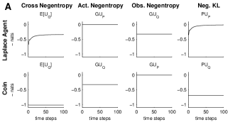
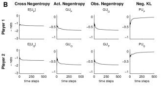
Figure 1: (A) Entropy dynamics of a Laplace agent interacting with a coin of bias $0.9$. The Laplace agent learns to predict the coin’s behavior as can be seen in the decrease of the KL-divergence and the cross entropy. Since the Laplace agent acts deterministically its action entropy is always zero. Its observation entropy equals the action entropy of the coin. The coin does not change its behavior, which can be seen from the flat entropy curves. (B) Entropy dynamics of two adaptive agents playing matching pennies. Both agents follow smooth fictitious play. They converge to uniform random policies, which means that their action negentropies converge to $\log(2)$. Both agents learn the probability distribution of the other agent, as can be seen in the decrease of the KL-divergences.

One of the most interesting aspects of the information-theoretic formulation of utility is that it can be applied both to control problems (where an agent acts in a non-adaptive environment) and to game theoretic problems (where two possibly adaptive agents interact). In the following we apply the proposed utility measures to two simple toy examples from these two areas. In the first example, an adaptive agent interacts with a biased coin (the non-adaptive agent) and tries to predict the next outcome of the coin toss, which is either ‘Head’ (H) or ‘Tail’ (T). In the second example two adaptive agents interact playing the matching pennies game. One player has to match her action with the other player (HH or TT), while the other player has to unmatch (TH or HT). All agents have the same sets of possible observations and actions which are the binary sets $\mathcal{O}=\{\mathrm{H},\mathrm{T}\}$ and $\mathcal{A}=\{\mathrm{H},\mathrm{T}\}$.

Example 1.

The non-adaptive agent is a biased coin. Accordingly, the coin’s action probability is given by its bias and was set to $\mathbf{Q}(o=\mathrm{H})=0.9$. The coin does not have any biased expectations about its observations, so we set $\mathbf{Q}(a=\mathrm{H})=0.5$. The adaptive agent is given by the Laplace agent whose expectations over observed coin tosses follows the predictive distribution $\mathbf{P}(o=\mathrm{H}|t,n)=(n+1)/(t+2)$, where $t$ is the number of coin tosses observed so far and $n$ is the number of observed Heads. Based on this estimator the Laplace agent chooses its action deterministically according to $\mathbf{P}(a=\mathrm{H}|t,n)=\Theta(\frac{n+1}{t+2}-\frac{1}{2})$, where $\Theta(\cdot)$ is the Heaviside step function. From these distributions the full probability over interaction sequences can be computed. Figure 1A shows the entropy dynamics for a typical single run. The Laplace agent learns the distribution of the coin tosses, i.e. the KL decreases to zero. The negative cross-entropy stabilizes at the value of the observation entropy that cannot be further reduced. The entropy dynamics of the coin do not show any modulation.

Example 2.

The two agents are modeled based on smooth fictitious play [Fudenberg and Kreps, 1993]. Both players keep count of the empirical frequencies of Head and Tail respectively. Therefore, each player $i$ stores the quantities $\kappa_{i}^{(1)}=n_{i}$ and $\kappa_{i}^{(2)}=t-n_{i}$ where $t$ is the number of moves observed so far, $n_{1}$ is the number of Heads observed by Player 1 and $n_{2}$ is the number of Heads observed by Player 2. The probability distributions $\mathbf{P}(o=\mathrm{H}|t,n_{1})=\gamma_{1}$ and $\mathbf{Q}(a=\mathrm{H}|t,n_{2})=\gamma_{2}$ over inputs is given by these empirical frequencies through $\gamma_{i}=\kappa_{i}/\sum_{i}\kappa_{i}$. The action probabilities are computed according to a sigmoid best-response function $\mathbf{P}(a=\mathrm{H}|t,n_{1})=1/(1+\exp(-\alpha(\gamma_{1}-0.5)))$, and $\mathbf{Q}(o=\mathrm{H}|t,n_{2})=1/(1+\exp(-\alpha(0.5-\gamma_{2})))$ respectively in case of Player 2 that has to unmatch. This game has a well-known equilibrium solution that is a mixed strategy Nash equilibrium where both players act randomly. Both action and observation entropies converge to the value $\log(2)$. Interestingly, the information-theoretic utility as computed by the cross-entropy takes the action entropy into account. Compare Figure 1B.

Conclusion

Based on three simple desiderata we propose that rewards can be measured in terms of information content and that, consequently, the entropy satisfies properties characteristic of a utility function. Previous theoretical studies have reported structural similarities between entropy and utility functions, see e.g. [Candeal, 2001], and recently, relative entropy has even been proposed as a measure of utility in control systems [Todorov, 2009, Kappen et al., 2009, Ortega and Braun, 2008]. The contribution of this paper is to derive axiomatically a precise relation between rewards and information value and to apply it to coupled I/O systems.

The utility functions that we have derived can be conceptualized as path utilities, because they assign a utility value to an entire history. This is very similar to the path integral formulation in quantum mechanics where the utility of a path is determined by the classic action integral and the probability of a path is also obtain by taking the exponential of this ‘utility’ [Feynman and Hibbs, 1965]. In particular, we obtain the (cumulative time-averaged) cross entropy as a utility function when an agent is coupled to an environment. This utility function not only takes into account the KL-divergence as a measure of learning, but also the action entropy. This is interesting, because in most control problems controllers are designed to be deterministic (e.g. optimal control theory) in response to a known and stationary environment. If, however, the environment is not stationary and in fact adaptive as well, then it is a well-known result from game theory that optimal strategies might be randomized. The utility function that we are proposing might indeed allow quantifying a trade-off between reducing the KL and reducing the action entropy. In the future it will therefore be interesting to investigate this utility function in more complex interaction systems.

Appendix A Appendix

Entropy functionals

Entropy: Let $\mathbf{P\!r}$ be a probability distribution over $\mathcal{X}\times\mathcal{Y}$. Define the (average conditional) entropy [Shannon, 1948] as

$$\mathbf{H}[\mathbf{P\!r}(x|y)]\equiv-\sum_{x,y}\mathbf{P\!r}(x,y)\ln\mathbf{P\!r}(x|y).$$

Relative Entropy: Let $\mathbf{P\!r}_{1}$ and $\mathbf{P\!r}_{2}$ be two probability distributions over $\mathcal{X}\times\mathcal{Y}$. Define the (average conditional) relative entropy [Kullback and Leibler, 1951] as

$$\mathbf{KL}[\mathbf{P\!r}_{1}(x|y)\|\mathbf{P\!r}_{2}(x|y)]\equiv\sum_{x,y}\mathbf{P\!r}_{1}(x,y)\ln\frac{\mathbf{P\!r}_{1}(x|y)}{\mathbf{P\!r}_{2}(x|y)}.$$

Proof of Theorem 1

Proof.

Let the function $g$ be such that $g(\mathbf{P\!r}(x))=\mathbf{r}(x)$. Let $x_{1},x_{2},\ldots,x_{n}\in\mathcal{F}$ be a sequence of events, such that $\mathbf{P\!r}(x_{1})=\mathbf{P\!r}(x_{i}|x_{<i})>0$ for all $i=2,\ldots,n$. We have $\mathbf{P\!r}(x_{1},\ldots,x_{n})=\prod_{i}\mathbf{P\!r}(x_{i}|x_{<i})=\mathbf{P\!r}(x_{1})^{n}$. Since $\mathbf{P\!r}(x)>\mathbf{P\!r}(x^{\prime})\Leftrightarrow\mathbf{r}(x)>\mathbf{r}(x^{\prime})$ for any $x,x^{\prime}\in\mathcal{F}$, then $\mathbf{P\!r}(x)=\mathbf{P\!r}(x^{\prime})\Leftrightarrow\mathbf{r}(x)=\mathbf{r}(x^{\prime})$, and thus $\mathbf{P\!r}(x_{1})=\mathbf{P\!r}(x_{i}|x_{<i})\Leftrightarrow\mathbf{r}(x_{1})=\mathbf{r}(x_{i}|x_{<i})$ for all $i=2,\ldots,n$. This means, $\mathbf{r}(x_{1},\ldots,x_{n})=n\mathbf{r}(x_{i})$. But $g(\mathbf{P\!r}(x_{1},\ldots,x_{n}))=\mathbf{r}(x_{1},\ldots,x_{n})$, and hence $g(\mathbf{P\!r}(x_{1})^{n})=n\mathbf{r}(x_{1})$. Similarly, for a second sequence of events $y_{1},y_{2},\ldots,y_{m}\in\mathcal{F}$ with $\mathbf{P\!r}(y_{1})=\mathbf{P\!r}(y_{i}|y_{<i})>0$ for all $i=1,\ldots,m$, we have $g(\mathbf{P\!r}(y_{1})^{n})=n\mathbf{r}(y_{1})$.

The rest of the argument parallels Shannon’s entropy theorem [Shannon, 1948]. Define $p=\mathbf{P\!r}(x_{1})$ and $q=\mathbf{P\!r}(y_{1})$. Choose $n$ arbitrarily high to satisfy $q^{m}\leq p^{n}<q^{m+1}$. Taking the logarithm, and dividing by $n\log q$ one obtains

$$\frac{m}{n}\leq\frac{\log p}{\log q}<\frac{m}{n}+\frac{1}{n}\quad\Leftrightarrow\quad\Bigl{|}\frac{m}{n}-\frac{\log p}{\log q}\Bigr{|}<\varepsilon,$$

where $\varepsilon>0$ is arbitrarily small. Similarly, using $g(p^{n})=n\,g(p)$ and the monotonicity of $g$, we can write $m\,g(q)\leq n\,g(p)<(m+1)\,g(q)$ and thus

$$\frac{m}{n}\leq\frac{g(p)}{g(q)}<\frac{m}{n}+\frac{1}{n}\quad\Leftrightarrow\quad\Bigl{|}\frac{m}{n}-\frac{g(p)}{g(q)}\Bigr{|}<\varepsilon,$$

where $\varepsilon>0$ is arbitrarily small. Combining these two inequalities, one gets

$$\Bigl{|}\frac{\log p}{\log q}-\frac{g(p)}{g(q)}\Bigr{|}<2\varepsilon,$$

which, fixing $q$, gives $\mathbf{r}(p)=g(p)=k\log p$, where $k>0$. This holds for any $x_{1}\in\mathcal{F}$ with $\mathbf{P\!r}(x_{1})>0$. ∎

Proof of Theorem 2

Proof.

For all $\omega,\omega^{\prime}\in\Omega$, $d(\omega)>d(\omega^{\prime})\Leftrightarrow\alpha d(\omega)+\beta>\alpha d(\omega^{\prime})+\beta\Leftrightarrow\mathbf{r}(\{\omega\})>\mathbf{r}(\{\omega^{\prime}\})$ because the affine transformation is positive. Now, the induced probability over $\mathscr{P}(\Omega)$ has atoms $\{\omega\}$ with probabilities $\mathbf{P\!r}(\{\omega\})=e^{\mathbf{r}(\{\omega)\}}\geq 0$ and is normalized:

$$\sum_{\omega\in\Omega}e^{\mathbf{r}(\{\omega\})}=\sum_{\omega\in\Omega}e^{\alpha d(\{\omega\})+\beta}=\frac{\sum_{\omega\in\Omega}e^{\alpha d(\omega)}}{\sum_{\omega\in\Omega}e^{\alpha d(\omega)}}=1.$$

Since knowing $\mathbf{P\!r}(\{\omega\})$ for all $\omega\in\Omega$ determines the measure for the whole field $\mathscr{P}(\Omega)$, $(\Omega,\mathscr{P}(\Omega),\mathbf{P\!r})$ is a probability space. ∎

Proof of Proposition 2

Proof.

(i) Since $-\infty<\mathbf{r}(x_{\tau}|x_{<\tau})\leq 0$ for all $\tau$, then $-\infty<\frac{1}{t}\sum_{\tau=1}^{t}\mathbf{r}(x_{\tau}|x_{<\tau})=\mathbf{U}(x_{\leq t})\leq 0$ for all $t$. (ii) Write $\mathbf{P\!r}(x_{\leq t})$ as

$$\mathbf{P\!r}(x_{\leq t}) =\prod_{\tau=1}^{t}\mathbf{P\!r}(x_{\tau}|x_{<\tau})=\prod_{\tau=1}^{t}\exp\Bigl{(}\mathbf{r}(x_{\tau}|x_{<\tau})\Bigr{)}$$

$$=\exp\Bigl{(}\sum_{\tau=1}^{t}\mathbf{r}(x_{\tau}|x_{<\tau})\Bigr{)}=\exp\Bigl{(}t\cdot\mathbf{U}(x_{\leq t})\Bigr{)}.$$

(iii) $\mathbf{E}[\mathbf{U}(x_{\leq t})]=\sum_{x_{\leq t}}\mathbf{P\!r}(x_{\leq t})\mathbf{U}(x_{\leq t})=\sum_{x_{\leq t}}\mathbf{P\!r}(x_{\leq t})\frac{1}{t}\mathbf{r}(x_{\leq t})=-\frac{1}{t}\mathbf{H}[\mathbf{P\!r}(x_{\leq t})]$, where we have applied (ii) in the second equality and $\mathbf{r}(\cdot)=\ln(\mathbf{P\!r}(\cdot))$ in the third equality. ∎

Proof of Theorem 3

Proof.

This proof is done by straightforward calculation. First note that

$$\mathbf{G}(\underline{ao}_{\leq t}) =\prod_{\tau=1}^{t}\mathbf{P}(a_{\tau}|\underline{ao}_{<\tau})\mathbf{Q}(o_{\tau}|\underline{ao}_{<\tau}a_{\tau})$$

$$=\mathbf{P}(a_{\leq t}|o_{<t})\mathbf{Q}(o_{\leq t}|a_{\leq t}),$$

which is obtained by applying multiple times the chain rule for probabilities and noting that the probability of a symbol is fully determined by the previous symbols. Similarly $\mathbf{P}(\underline{ao}_{\leq t})=\mathbf{P}(a_{\leq t}|o_{<t})\mathbf{P}(o_{\leq t}|a_{\leq t})$ is obtained. We calculate here $\mathbf{E}[\mathbf{r}_{\mathbf{P}}(\underline{ao}_{\leq t})]$. The calculation for $\mathbf{E}[\mathbf{r}_{\mathbf{G}}(\underline{ao}_{\leq t})]$ and $\mathbf{E}[\mathbf{r}_{\mathbf{Q}}(\underline{ao}_{\leq t})]$ are omitted because they are analogous.

$$\mathbf{E}[\mathbf{r}_{\mathbf{P}}(\underline{ao}_{\leq t})] \stackrel{{\scriptstyle(a)}}{{=}}\sum_{\underline{ao}_{\leq t}}\mathbf{G}(\underline{ao}_{\leq t})\ln\mathbf{P}(\underline{ao}_{\leq t})$$

$$\stackrel{{\scriptstyle(b)}}{{=}}\sum_{\underline{ao}_{\leq t}}\mathbf{G}(\underline{ao}_{\leq t})\Bigl{(}\ln\mathbf{P}(a_{\leq t}|o_{<t})+\ln\mathbf{P}(o_{\leq t}|a_{\leq t})\Bigr{)}$$

$$\stackrel{{\scriptstyle(c)}}{{=}}\sum_{\underline{ao}_{\leq t}}\mathbf{G}(\underline{ao}_{\leq t})\Bigl{(}\ln\mathbf{P}(a_{\leq t}|o_{<t})+\ln\mathbf{P}(o_{\leq t}|a_{\leq t})$$

$$\qquad+\ln\mathbf{Q}(o_{\leq t}|a_{\leq t})-\ln\mathbf{Q}(o_{\leq t}|a_{\leq t})\Bigr{)}$$

$$\stackrel{{\scriptstyle(d)}}{{=}}-\mathbf{H}[\mathbf{P}(a_{\leq t}|o_{<t})]-\mathbf{H}[\mathbf{Q}(o_{\leq t}|a_{\leq t})]$$

$$\qquad-\mathbf{KL}[\mathbf{Q}(o_{\leq t}|a_{\leq t})\|\mathbf{P}(o_{\leq t}|a_{\leq t})].$$

Equality (a) follows from the definition of expectations and the relation between rewards and probabilities. In (b) we separate the term in the logarithm into the action and observation part. In (c) we add and subtract the term $\mathbf{Q}(o_{\leq t}|a_{\leq t})$ in the logarithm. Equality (d) follows from the algebraic manipulation of the terms and from identifying the entropy terms, noting that $\mathbf{G}(\underline{ao}_{\leq t})=\mathbf{P}(a_{\leq t}|o_{<t})\mathbf{Q}(o_{\leq t}|a_{\leq t})$. ∎

References

- Candeal [2001] De Miguel J.R. Indur in E. Mehta G.B. Candeal, J.C. Utility and entropy. Economic Theory, 17:233–238, 2001.
- Feynman and Hibbs [1965] R.P. Feynman and A.R. Hibbs. Quantum Mechanics and Path Integrals. McGraw-Hill, 1965.
- Fishburn [1982] P.C. Fishburn. The Foundations of Expected Utility. D. Reidel Publishing, Dordrecht, 1982.
- Fudenberg and Kreps [1993] D. Fudenberg and D.M. Kreps. Learning mixed equilibria. Games and Economic Behavior, 5:320–367, 1993.
- Kappen et al. [2009] B. Kappen, V. Gomez, and M. Opper. Optimal control as a graphical model inference problem. arXiv:0901.0633, 2009.
- Kullback and Leibler [1951] S. Kullback and R.A. Leibler. On information and sufficiency. The Annals of Mathematical Statistics, 22(1):79–86, mar 1951. ISSN 0003-4851.
- MacKay [2003] D.J.C. MacKay. Information Theory, Inference, and Learning Algorithms. Cambridge University Press, 2003.
- Ortega and Braun [2008] P.A. Ortega and D.A. Braun. A minimum relative entropy principle for learning and acting. arXiv:0810.3605, 2008.
- Russell and Norvig [1995] S. Russell and P. Norvig. Artificial Intelligence: A Modern Approach. Prentice-Hall, Englewood Cliffs, NJ, 1st edition edition, 1995.
- Shannon [1948] C. E. Shannon. A mathematical theory of communication. Bell System Technical Journal, 27:379–423 and 623–656, Jul and Oct 1948.
- Todorov [2009] E. Todorov. Efficient computation of optimal actions. Proceedings of the National Academy of Sciences U.S.A., 106:11478–11483, 2009.