High-Order Coupled Cluster Method (CCM) Formalism 2 – “Generalised” Expectation Values: Spin-Spin Correlation Functions for Frustrated and Unfrustrated 2D Antiferromagnets

Abstract

Recent developments of high-order CCM have been to extend existing formalism and codes to $s\geq\frac{1}{2}$ for both the ground and excited states. In this article, we describe how “generalised” expectation values for a wide range of one- and two-body spin operators may also be determined using existing the CCM code for the ground state. We present new results for the spin-spin correlation functions of the spin-half square- and triangular-lattice antiferromagnets by using the LSUB$m$ approximation. We show that the absolute values of the spin-spin correlation functions $|\langle\bf{s}(0).\bf{s}(r)\rangle|$ converge with increasing approximation level for both lattices. We believe that the LSUB$m$ approximation provides reasonable results for the correlation functions for lattice separations roughly of order $r\approx m$ for the square lattice. We compare qualitatively our results for the square lattice to those results of quantum Monte Carlo (QMC) and we see that good correspondence is observed. Indeed as seen by QMC, the spin-spin correlation function initially decays strongly with $|r|$ before becoming constant for larger values of $|r|$. CCM results are also compared to results of exact diagonalisations for both lattices. ED results demonstrate a strong finite-size effects at lattice separations $r=L/2$ (where $N=L\times L$) for both lattices. The behaviour of the correlation function for the triangular lattice is qualitatively similar to that of the square lattice, namely, that it decays strongly at first before becoming constant. This is in keeping with the behaviour of both models, which are believed strongly to be Néel-ordered from approximate studies. The CCM has been shown many times to provide consistently good results for the ground-state energy and sublattice magnetisation of a wide range of quantum spin models. Here we have shown that the CCM also provides good results for the spin-spin correlation function.

I Introduction

The coupled cluster method (CCM) refc1 ; refc2 ; refc3 ; refc4 ; refc5 ; refc6 ; refc7 ; refc8 ; refc9 is a well-known method of quantum many-body theory (QMBT). The CCM has been applied with much success in order to study quantum magnetic systems at zero temperature (see Refs. ccm1 ; ccm2 ; ccm999 ; ccm3 ; ccm4 ; ccm5 ; ccm6 ; ccm7 ; ccm8 ; ccm9 ; ccm10 ; ccm11 ; ccm12 ; ccm13 ; ccm13a ; ccm14 ; ccm15 ; ccm16 ; ccm17 ; ccm18 ; ccm19 ; ccm19a ; ccm20 ; ccm21 ; ccm22 ; ccm23 ; ccm24 ; ccm24a ; ccm26 ; ccm27 ; ccm27a ; ccm28 ; ccm29 ; ccm30 ; ccm31 ; ccm32 ; ccm33 ; ccm34 ; ccm35 ; ccm36 ; ccm37 ; ccm38 ; ccm39 ). In particular, the use of computer-algebraic implementations ccm12 ; ccm15 ; ccm20 ; ccm39 of the CCM has been found to be very effective with respect to these spin-lattice problems. Recent developments of high-order CCM formalism and codes have been to treat systems with spin quantum number of $s\geq\frac{1}{2}$ for both the ground and excited states ccm39 . In this article, we show how these ground-state formalism and codes may also be used directly to find “generalised” expectation values; that is, expectation values for a wide range of one- or two-body spin operator that are defined prior to the CCM calculation.

We apply the CCM to the spin-half Heisenberg model on the square and triangular lattices. The Hamiltonian is specified as follows,

$$H=\sum_{\langle i,j\rangle}{\bf s}_{i}~{}\cdot~{}{\bf s}_{j}~{}~{},$$ (1)

where the sum on $\langle i,j\rangle$ counts all nearest-neighbour pairs once. The ground states of all of the cases considered here are classically ordered, albeit by a reduced amount due to quantum fluctuations. Indeed, the best estimates of the amount of classical ordering of the square lattice case from approximate methods are 61$\%$ from CCMccm28 , 61.4$\%$ from quantum Monte Carlo studiesqmc3 , 61.4$\%$ from series expansionsseries3 , 61.38$\%$ from spin-wave theoryswt3 , and 63.4$\%$ from exact diagonalisationsed1 . Good results for the spin-spin correlation function of the spin-half square-lattice Heisenberg antiferromagnet were found using quantum Monte Carlo in Ref. qmc4 on lattices of size up to $N=L\times L$, where $L=\{16,22,32\}$. They observed that the correlation functions decayed with separation $r$. However, they also saw finite-size effects, indicated by cusp-like behaviour in these correlation functions, at distances given by $L/2$. Exact diagonalisations have also been carried out for the correlation function of the square lattice ed2 . For the spin-half triangular-lattice antiferromagnet, the best estimates of the amount of classical ordering are 41$\%$ from quantum Monte Carlo studiesqmc2 , 40$\%$ from series expansionsseries2 , 39$\%$ from exact diagonalisationsed1 , and 40$\%$ from previous CCM calculationsccm28 . Very few results for the spin-spin correlation functions of the triangular lattice seem to exist apart from results of exact diagonalisations (e.g., see edt ).

II Method

The details of the practical application of high-order coupled cluster method (CCM) formalism to lattice quantum spin systems are given in Refs. ccm12 ; ccm15 ; ccm20 ; ccm26 ; ccm39 and also in the appendices to this article. However, we point out now that the ket and bra ground-state energy eigenvectors, $|\Psi\rangle$ and $\langle\tilde{\Psi}|$, of a general many-body system described by a Hamiltonian $H$, are given by

$$H|\Psi\rangle=E_{g}|\Psi\rangle\;;\;\;\;\langle\tilde{\Psi}|H=E_{g}\langle\tilde{\Psi}|\;.$$ (2)

Furthermore, the ket and bra states are parametrized within the single-reference CCM as follows:

$$|\Psi\rangle={\rm e}^{S}|\Phi\rangle\; \;\;\;S=\sum_{I\neq 0}{\cal S}_{I}C_{I}^{+}\;,$$ ;

$$\langle\tilde{\Psi}|=\langle\Phi|\tilde{S}{\rm e}^{-S}\; \;\;\;\tilde{S}=1+\sum_{I\neq 0}\tilde{{\cal S}}_{I}C_{I}^{-}\;.$$ ; (3)

One of the most important features of the CCM is that one uses a single model or reference state $|\Phi\rangle$ that is normalized. We note that the parametrisation of the ground state has the normalization condition for the ground-state bra and ket wave functions ($\langle\tilde{\Psi}|\Psi\rangle\equiv\langle\Phi|\Phi\rangle=1$). The model state is required to have the property of being a cyclic vector with respect to two well-defined Abelian subalgebras of multi-configurational creation operators $\{C_{I}^{+}\}$ and their Hermitian-adjoint destruction counterparts $\{C_{I}^{-}\equiv(C_{I}^{+})^{\dagger}\}$. The interested reader is referred to the Appendices and to Ref. ccm39 for more information regarding how the CCM problem is solved for.

Here, we use the classical ground state as the model state. For the square lattice, this is the Néel state in which neighbouring spins are antiparallel, and, for the triangular lattice, this a Néel-lke state in which neighbouring spins on three sublattices are at 120^∘ to each other. For the square lattice, we perform a rotation of the local axes of the up-pointing spins by 180^∘ about the $y$-axis. The transformation is described by,

$$s^{x}\;\rightarrow\;-s^{x},\;s^{y}\;\rightarrow\;s^{y},\;s^{z}\;\rightarrow\;-s^{z}\;.$$ (4)

The model state now appears $mathematically$ to consist of purely down-pointing spins. In terms of the spin raising and lowering operators $s_{k}^{\pm}\equiv s_{k}^{x}\pm{\rm i}s_{k}^{y}$ the Hamiltonian may be written in these local axes as,

$$H=-\frac{1}{2}\sum_{\langle i,j\rangle}^{N}\;\biggl{[}\;s_{i}^{+}s_{j}^{+}+s_{i}^{-}s_{j}^{-}+2s_{i}^{z}s_{j}^{z}\;\biggr{]}\;,$$ (5)

where the sum on $\langle i,j\rangle$ again counts all nearest-neighbour pairs once on the square lattice. Again, the classical ground-state of the Heisenberg model of Eq. (1) for the triangular lattice is the Néel-like state where all spins on each sublattice are separately aligned (all in the $xz$-plane, say). The spins on sublattice A are oriented along the negative z-axis, and spins on sublattices B and C are oriented at $+120^{\circ}$ and $-120^{\circ}$, respectively, with respect to the spins on sublattice A. We again rotate the local spin axes of those spins on the different sublattices. Specifically, we leave the spin axes on sublattice A unchanged, and we rotate about the $y$-axis the spin axes on sublattices B and C by $-120^{\circ}$ and $+120^{\circ}$ respectively,

$$s_{B}^{x}\rightarrow-\frac{1}{2}s_{B}^{x}-\frac{\sqrt{3}}{2}s_{B}^{z}\;\; \;\;s_{C}^{x}\rightarrow-\frac{1}{2}s_{C}^{x}+\frac{\sqrt{3}}{2}s_{C}^{z}\;\;,$$ ;

$$s_{B}^{y}\rightarrow s_{B}^{y}\;\; \;\;s_{C}^{y}\rightarrow s_{C}^{y}\;\;,$$ ;

$$s_{B}^{z}\rightarrow\frac{\sqrt{3}}{2}s_{B}^{x}-\frac{1}{2}s_{B}^{z}\;\; \;\;s_{C}^{z}\rightarrow-\frac{\sqrt{3}}{2}s_{C}^{x}-\frac{1}{2}s_{C}^{z}\;\;.$$ ; (6)

Once again, the model state now appears to consist of purely down-pointing spins. We may rewrite Eq. (1) in terms of spins defined in these local quantisation axes for the triangular lattice, such that

$$H=\sum_{\langle i\rightarrow j\rangle}\Bigl{\{} -{1\over 2}s_{i}^{z}s_{j}^{z}+\frac{\sqrt{3}}{4}\left(s_{i}^{z}s_{j}^{+}+s_{i}^{z}s_{j}^{-}-s_{i}^{+}s_{j}^{z}-s_{i}^{-}s_{j}^{z}\right)$$ (7)

$$+\frac{1}{8}\left(s_{i}^{+}s_{j}^{-}+s_{i}^{-}s_{j}^{+}\right)-\frac{3}{8}\left(s_{i}^{+}s_{j}^{+}+s_{i}^{-}s_{j}^{-}\right)\Bigl{\}}\;\;.$$

We note that the summation in Eq. (7) again runs over nearest-neighbour bonds, but now also with a directionality indicated by $\langle i\rightarrow j\rangle$, which goes from A to B, B to C, and C to A.

The CCM formalism is exact in the limit of inclusion of all possible multi-spin cluster correlations within $S$ and $\tilde{S}$, although this is usually impossible to achieve practically. Hence, we generally make approximations in both $S$ and $\tilde{S}$. The three most commonly employed approximation schemes previously utilised have been: (1) the SUB$n$ scheme, in which all correlations involving only $n$ or fewer spins are retained, but no further restriction is made concerning their spatial separation on the lattice; (2) the SUB$n$-$m$ sub-approximation, in which all SUB$n$ correlations spanning a range of no more than $m$ adjacent lattice sites are retained; and (3) the localised LSUB$m$ scheme, in which all multi-spin correlations over all distinct locales on the lattice defined by $m$ or fewer contiguous sites are retained. Another important feature of the method is that the bra and ket states are not always explicitly constrained to be Hermitian conjugates when we make such approximations, although the important Helmann-Feynman theorem is always preserved. We remark that the CCM provides results in the infinite-lattice limit $N\rightarrow\infty$ from the outset.

In this article, we wish to determine the spin-spin correlation functions $|\langle\bf{s}(0).\bf{s}(r)\rangle|$ as a function of lattice separation $|r|$ for the (unfrustrated) square-lattice and (frustrated) triangular-lattice antiferromagnets. We must take into account the rotation of the local spin axes, although this proceeds in exactly the same manner as for the Hamiltonian above. Again, we remark that the manner in which high-order CCM may be solved has been discussed in Ref. ccm39 . The manner in which the ground-state CCM ket- and bra-state equations are solved is discussed in the Appendix to this article. In particular, the method by which “generalised expectation values” for a variety of one- and two-body spin operators may be obtained is explained in the appendices.

III Results

The results for the absolute values of the spin-spin correlation functions for the (unfrustrated) spin-half square-lattice antiferromagnet using the LSUB$m$ approximation with $m=\{2,4,6,8\}$ are shown in Fig. 1. The LSUB$m$ results are in very good mutual agreement for small lattice separations for different values of $m$. Indeed, LSUB$m$ results are clearly converging with increasing levels of approximation. Furthermore, we see that LSUB6 and LSUB8 correspond reasonably well with each other up to $r\stackrel{{\scriptstyle\sim}}{{<}}5$. From Fig. 1 (as a “rule of thumb” only), we believe LSUB$m$ results ought to provide reasonable results to lattice separations approximately of order $m$ for the square lattice.

CCM results are also compared to those results of exact diagonalisations (ED) ed2 in Fig. 1. However, we see that we obtain good correspondence only for very small lattice separations $r<3$. (We note that $N=40$ is at the current upper limit for ED of computational tractability.) However, the agreement between ED and CCM becomes rapidly worse for lattice separation $r\geq 3$. This disparity can be understood by considering results of quantum Monte Carlo (QMC) of Ref. qmc4 for the spin-spin correlation function, which were carried out for for much larger lattices of size of $N=L\times L$, where $L=\{16,22,32\}$. Indeed, we find good correspondence qualitatively (i.e., compared by by eye only) between the LSUB8 results of Fig. 1 and those QMC results for the largest lattice $N=32\times 32$ of Fig. 3a in Ref. qmc4 . Furthermore, the authors of Ref. qmc4 noted a strong cusp-like behaviour was seen in the spin-spin correlation function at lattice separations of $L/2$ due to finite-lattice effects. This is also seen in Fig. 1 for the ED results at $r=3$, although this cusp may be exacerbated by a small “kink” in the “true” spin-spin correlation function that occurs at this point anyway (as seen in both CCM and QMC results). Interestingly, we see from Fig. 3b of Ref. qmc4 that the accuracy of QMC results for the spin-spin correlation functions becomes more problematic (again as a “rule of thumb” only) for separations of order $r\stackrel{{\scriptstyle\sim}}{{>}}L/2$ for a given lattice size $N=L\times L$. Hence, we might also reasonably expect that results of ED might only be good for separations of $r<3$ for lattices of size $N=36$ and $n=40$. Indeed, we note that ED agrees well with highly converged CCM results (and incidentally QMC results of Fig. 3a in Ref. qmc4 – again comparing by eye only) in this region.

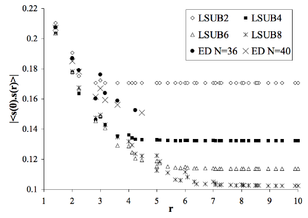
Figure 1: CCM results for the absolute values of the spin-spin correlation function for the spin-half square-lattice antiferromagnet using the LSUB$m$ approximation with $m=\{2,4,6,8\}$. CCM results are compared to those results of exact diagonalisations (ED) with $N=36,40$ ed2 .

The author of the QMC calculations in Ref. qmc4 noted that: “to good approximation, the two-point function depends only on $|r|$.” As also noted in Ref. qmc4 , the long-range behaviour of correlation function gives a constant, thus indicating a long-range ordered ground state. We see this also at all levels of approximation as shown in Fig. 1. Results ccm15 for the sublattice magnetisation have shown that extrapolation of the CCM LSUB$m$ results gives good correspondence to the results of QMC, as noted above, where both methods indicate from the sublattice magnetisation that approximately 61$\%$ of the classical Néel order remains in the quantum limit. Finally, the author of Ref. qmc4 remarked that the approach to the constant for larger separations could be fitted by either an exponential or power-law form. We tried both for the LSUB8 data with $r\leq 8$ and found nothing to contradict this statement, although the power-law decay seemed to work better (i.e., had a lower residual error) that the exponential law. The residual sum-of-squares error for the power-law form was 0.0015 and for the exponential form was 0.0034. Fits of these forms to the LSUB8 data were carried out using the R statistics language: http://cran.r-project.org/.

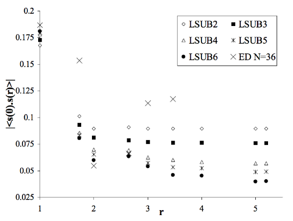
Figure 2: CCM results for the absolute values of the spin-spin correlation function for the spin-half triangular-lattice antiferromagnet using the LSUB$m$ approximation with $m=\{2,3,4,5,6\}$. CCM results are compared to those results of exact diagonalisations (ED) edt with $N=36$.

The results for the (frustrated) spin-half square-lattice antiferromagnet using the LSUB$m$ approximation with $m=\{2,3,4,5,6\}$ are shown in Fig. 2. Again, LSUB$m$ results are clearly converging with increasing levels of approximation, and again they are in very good mutual agreement for small lattice separations. CCM results are again compared to results of ED for$N=36$ (e.g., see Ref. edt ), and again good agreement is found for very small lattice separations ($r<3$). Another strong cusp-like behaviour is seen in ED results for the spin-spin correlation function for $r\approx 3$. Again, it is highly likely that this is primarily due to finite-size effects. Indeed, we see that CCM results for $r\geq 3$ are quite different to those of ED. Furthermore, CCM LSUB$m$ results initially decay strongly and then tend to a constant value for larger lattice separations. The behaviour of the correlation function for the triangular lattice is broadly similar to that of the square lattice. Again, extrapolation of LSUB$m$ results ccm28 for the sublattice magnetisation demonstrate that the spin-half triangular lattice antiferromagnet is Néel ordered. For LSUB6 with $r\leq 5.5$, we found that the initial decay of the correlation function for CCM data in this case could be fitted well by either an exponential or power-law form (for both forms, residual sum-of-squares: 0.0002).

IV conclusions

We have presented new formalism for the CCM in order to form “generalised” expectation values for a wide range of terms in the spin Hamiltonian. This is particularly useful for “high-order” CCM thecode . We have applied this approach in order to determine the spin-spin correlation functions for frustrated and unfrustrated 2D antiferromagnets, namely, the spin-half triangular- and square-lattice Heisenberg models. We found good correspondence of CCM with results of quantum Monte Carlo (QMC) for the square-lattice antiferromagnet. A strong cusp-like behaviour was noted in exact diagonalisation (ED) results for the correlation function at a lattice separation $L/2$ for a lattice of size $N=L\times L$ for both lattices. This is a finite-size effect. A cusp in the spin-spin correlation function was also seen in QMC results at $r=L/2$ for a $N=L\times L$ lattice.

By contrast, this cusp was not seen in CCM results for either lattice at any value of $r$ at any level of LSUB$m$ approximation. Indeed, we note that CCM results are determined in the infinite-lattice limit ($N\rightarrow\infty$) from the outset. We believe that (as a “rule of thumb”) we obtain reasonable results for the correlation function up to separations of $r\approx m$ for the square lattice – even despite the fact that we are using a purely “localised” LSUB$m$ approximation scheme. LSUB$m$ results for the triangular lattice are clearly converging, and are in good mutual agreement for small lattice separations. For both lattices, CCM results for the correlation function decay strongly initially, although they become constant for larger values of $r$. Previous CCM results for the sublattice magnetisation ccm28 indicate that the spin-half Heisenberg models for the square and triangular lattices are Néel ordered, which agrees with the results of other approximate methods.

It is still fair to say that QMC results still generally provide the most accurate results for the unfrustrated Heisenberg model on lattices of two spatial dimensions. However, QMC is severely restricted by the “sign problem,” which is a consequence of frustration at $T=0$. The CCM has been shown ccm28 to provides good results for the ground-state properties of the spin-half triangular lattice antiferromagnet such as the ground-state energy and sublattice magnetisation. Here we have shown that the CCM also provides reasonable results for the spin-spin correlation function of the spin-half triangular lattice antiferromagnet. Finally, we note that CCM results indicate that the behaviour of the correlation function for the triangular lattice is broadly similar to that of the square lattice.

Appendix A CCM Formalism

We begin the description of the application of the CCM by noting that it may be proven from Eqs. (2) and (3) in a straightforward manner that the ket- and bra-state equations are thus given by

$$\langle\Phi|C_{I}^{-}{\rm e}^{-S}H{\rm e}^{S}|\Phi\rangle = 0,\;\;\forall I\neq 0\;\;;$$ (8)

$$\langle\Phi|\tilde{S}{\rm e}^{-S}[H,C_{I}^{+}]{\rm e}^{S}|\Phi\rangle = 0,\;\;\forall I\neq 0\;\;.$$ (9)

The index $I$ refers to a particular choice of cluster from the set of ($N_{F}$) fundamental clusters that are distinct under the symmetries of the crystallographic lattice and the Hamiltonian and for a given approximation scheme at a given level of approximation. We note that these equations are equivalent to the minimization of the expectation value of $\bar{H}=\langle\tilde{\Psi}|H|\Psi\rangle$ with respect to the CCM bra- and ket-state correlation coefficients $\{\tilde{{\cal S}}_{I},{\cal S}_{I}\}$. We note that Eq. (8) is equivalent to $\delta{\bar{H}}/\delta{\tilde{{\cal S}}_{I}}=0$, whereas Eq. (9) is equivalent to $\delta{\bar{H}}/\delta{{\cal S}_{I}}=0$. Furthermore, we note that Eq. (8) leads directly to simple form for the ground-state energy given by

$$E_{g}=E_{g}(\{{\cal S}_{I}\})=\langle\Phi|{\rm e}^{-S}H{\rm e}^{S}|\Phi\rangle\;\;.$$ (10)

The full set $\{{\cal S}_{I},\tilde{{\cal S}}_{I}\}$ provides a complete description of the ground state. For instance, an arbitrary operator $A$ will have a ground-state expectation value given as

$$\bar{A}\equiv\langle\tilde{\Psi}|A|\Psi\rangle=\langle\Phi|\tilde{S}{\rm e}^{-S}A{\rm e}^{S}|\Phi\rangle=\bar{A}\left(\{{\cal S}_{I},\tilde{{\cal S}}_{I}\}\right)\;.$$ (11)

The similarity transform of $A$ is given by,

$$\tilde{A}\equiv{\rm e}^{-S}A{\rm e}^{S}=A+[A,S]+{1\over 2!}[[A,S],S]+\cdots\;\;.$$ (12)

Appendix B High-Order CCM

The manner is which the ground-state problem is solved to high-orders of approximation via computational is provided in Ref. ccm39 . However, we note that use new “high-order CCM operators” that are formed purely of spin-raising operators with respect to the model state. The model state is taken to be a state in which all spins point in the downwards $z$-direction after some appropriate rotation of the local axes of the spins. This allows us to write one- and two-body spin operators in terms of these new high-order CCM operators. The problem inherent in Eq. (8) becomes one of pattern-matching the fundamental set of clusters in $C_{I}^{-}$ to the terms in the similarity transformed version of the Hamiltonian $e^{-S}He^{S}|\Phi\rangle$, where the $I$-th such equation is given by

$$E_{I}\equiv\langle\Phi|C_{I}^{-}e^{-S}He^{S}|\Phi\rangle=0~{}~{},\forall I\neq 0~{}~{}.$$ (13)

(Note that we assume that $\langle\Phi|C_{I}^{-}C_{I}^{+}|\Phi\rangle=1$ in the above equation). Specific terms in the Hamiltonian that may be used in the CCM code are: $s^{z}s^{z}$; $s^{+}s^{z}$; $s^{-}s^{z}$; $s^{z}s^{+}$; $s^{z}s^{-}$; $s^{+}s^{-}$; $s^{-}s^{+}$; $s^{+}s^{+}$; $s^{-}s^{-}$; $s^{+}$; $s^{-}$; $s^{z}$; and, $(s^{z})^{2}$. We now “pattern-match” the $C_{i}^{-}$ operators to those the relevant terms in the similarity transformed version of the Hamiltonian in order to form the CCM equations $E_{I}=0$ of Eq. (13) at a given level of approximation.

We now define the following new set of CCM bra-state correlation coefficients given by $x_{I}\equiv{\cal S}_{I}$ and $\tilde{x}_{I}\equiv N_{B}/N(l!)\nu_{I}\tilde{\cal S}_{I}$ and we assume again that $\langle\Phi|C_{I}^{-}C_{I}^{+}|\Phi\rangle=1$. Note that $N_{B}$ is the number of Bravais lattice sites. Note also that for a given cluster $I$ then $\nu_{I}$ is a symmetry factor which is dependent purely on the point-group symmetries (and not the translational symmetries) of the crystallographic lattice and that $l$ is the number of spin operators. We note that the factors $\nu_{I}$, $N$, $N_{B}$, and $(l!)$ never need to be explicitly determined. The CCM bra-state operator may thus be rewritten as

$$\tilde{S}\equiv 1+N\sum_{I=1}^{N_{F}}{\tilde{x}_{I}}C_{I}^{-}~{}~{},$$ (14)

such that we have a particularly simple form for $\bar{H}$, given by

$$\bar{H}=N\sum_{I=0}^{N_{F}}\tilde{x}_{I}E_{I}~{}~{},$$ (15)

where $\tilde{x}_{0}=1$. We note that the $E_{0}$ is defined by $E_{0}=\frac{1}{N}\langle\Phi|e^{-S}He^{S}|\Phi\rangle$ (and, thus, $E_{0}=\frac{1}{N}E_{g}$) and that $E_{I}$ is the $I$-th CCM ket-state equation defined by Eq. (13). The CCM ket-state equations are easily re-derived by taking the partial derivative of $\bar{H}/N$ with respect to $\tilde{x}_{I}$, where

$$\frac{\delta{(\bar{H}/N)}}{\delta\tilde{x}_{I}}(\equiv 0)=E_{I}~{}~{}.$$ (16)

We now take the partial derivative of $\bar{H}/N$ with respect to $x_{I}$ such that the bra-state equations take on a particularly simple form, given by

$$\frac{\delta{(\bar{H}/N)}}{\delta x_{I}}=\frac{\delta{E_{0}}}{\delta x_{I}}+\sum_{J=1}^{N_{F}}\tilde{x}_{J}\frac{\delta{E_{J}}}{\delta x_{I}}(\equiv 0)=\tilde{E}_{I}~{}~{}.$$ (17)

Appendix C Generalized Ground-State Expectation Values

The expectation value of a “generalized” spin operator that we shall call $A$ may be treated in an analogous manner to that of the expectation value of the Hamiltonian, given by $\bar{H}$. We write:

$$A_{I}=\langle\Phi|C_{I}^{-}e^{-S}Ae^{S}|\Phi\rangle$$ (18)

and with $C_{0}^{-}=1$. The similarity transform of $A$ is defined by Eq. (11). We may treat a wide range of one- and two-body spin operations. However, unlike the Heisenberg Hamiltonian of Eq. (1), we do not constrain $i$ and $j$ in the two-body terms to be only nearest-neighbors or next-nearest-neighbors. For example, we consider here the spin-spin correlation functions. The expectation value of the generalized (spin) operator may again be written in a particularly simple form as:

$$\bar{A} = \langle\tilde{\Psi}|A|\Psi\rangle~{}~{}$$

$$= N\sum_{I=0}^{N_{F}}{\tilde{x}_{I}}\langle\Phi|C_{I}^{-}e^{-S}Ae^{S}|\Phi\rangle~{}~{}$$

$$\Rightarrow\bar{A} = N\sum_{I=0}^{N_{F}}\tilde{x}_{I}A_{I}~{}~{},$$ (19)

where $\tilde{x}_{0}=1$ also and $A_{0}=\frac{1}{N}\langle\Phi|e^{-S}Ae^{S}|\Phi\rangle$. The same code used to find ground-state equations may be used to find the generalized expectation values. Again we note that the index $I$ in Eq. (19) runs from zero to $N_{F}$. Again, we note that factors such as $N_{B}$ or $\nu_{I}$ etc. do not need to be determined explicitly because they cancel because of the definition of $\{\tilde{x}_{I}\}$ given above. The techniques need to achieve a computational solution have been discussed extensively elsewhere, and the interested reader is referred to Refs. ccm12 ; ccm15 ; ccm20 ; ccm26 ; ccm39 for more information. However, clearly we see that the summation over all fundamental clusters involved in evaluating $\bar{A}$ is carried out readily once the ket- and bra-state equations of Eqs. (16) and (17) have been solved for.

References

- (1) F. Coester, Nucl. Phys. 7, 421 (1958); F. Coester and H. Kümmel, ibid. 17, 477 (1960).
- (2) J. Čižek, J. Chem. Phys. 45, 4256 (1966); Adv. Chem. Phys. 14, 35 (1969).
- (3) R.F. Bishop and K.H. Lührmann, Phys. Rev. B 17, 3757 (1978); ibid. 26, 5523 (1982).
- (4) H. Kümmel, K.H. Lührmann, and J.G. Zabolitzky, Phys Rep. 36C, 1 (1978).
- (5) J.S. Arponen, Ann. Phys. (N.Y.) 151, 311 (1983).
- (6) R.F. Bishop and H. Kümmel, Phys. Today 40(3), 52 (1987).
- (7) J.S. Arponen, R.F. Bishop, and E. Pajanne, Phys. Rev. A 36, 2519 (1987); ibid. 36, 2539 (1987); in: Condensed Matter Theories, Vol. 2, P. Vashishta, R.K. Kalia, and R.F. Bishop, eds. (Plenum, New York, 1987), p. 357.
- (8) R.J. Bartlett, J. Phys. Chem. 93, 1697 (1989).
- (9) R.F. Bishop, Theor. Chim. Acta 80, 95 (1991).
- (10) M. Roger and J.H. Hetherington, Phys. Rev. B 41, 200 (1990); Europhys. Lett. 11, 255 (1990).
- (11) R.F. Bishop, J.B. Parkinson, and Y. Xian, Phys. Rev. B 44, 9425 (1991).
- (12) R.F. Bishop, J.B. Parkinson, and Y. Xian, Phys. Rev. B 46, 880 (1992).
- (13) R.F. Bishop, J.B. Parkinson, and Y. Xian, J. Phys.: Condens. Matter 5, 9169 (1993).
- (14) D.J.J. Farnell and J.B. Parkinson, J. Phys.: Condens. Matter 6, 5521 (1994).
- (15) R.F. Bishop, R.G. Hale, and Y. Xian, Phys. Rev. Lett. 73, 3157 (1994).
- (16) Y. Xian, J. Phys.: Condens. Matter 6, 5965 (1994).
- (17) R. Bursill, G.A. Gehring, D.J.J. Farnell, J.B. Parkinson, T. Xiang, and C. Zeng, J. Phys.: Condens. Matter 7, 8605 (1995).
- (18) R.G. Hale. Ph.D. Thesis, UMIST, Manchester, United Kingdom (1995).
- (19) R.F. Bishop, D.J.J. Farnell, and J.B. Parkinson, J. Phys.: Condens. Matter 8, 11153 (1996).
- (20) D.J.J. Farnell, S.A. Krüger, and J.B. Parkinson, J. Phys.: Condens. Matter 9, 7601 (1997).
- (21) R.F. Bishop, Y. Xian, and C. Zeng, in: Condensed Matter Theories, Vol. 11, E.V. Ludeña, P. Vashishta, and R.F. Bishop, eds. (Nova Science, Commack, New York, 1996), p. 91.
- (22) C. Zeng, D.J.J. Farnell, and R.F. Bishop, J. Stat. Phys. 90, 327 (1998).
- (23) R.F. Bishop, D.J.J. Farnell, and J.B. Parkinson, Phys. Rev. B 58, 6394 (1998).
- (24) R.F. Bishop in Microscopic Many-Body Theories and Their Applications, Lecture Notes in Physics 510, J. Navarro and A. Polls, eds. Lecture Notes in Physics Vol. 510 (Springer-Verlag, Berlin, 1998), p. 1.
- (25) J. Rosenfeld, N.E. Ligterink, and R.F. Bishop, Phys. Rev. B 60, 4030 (1999).
- (26) R.F. Bishop, D.J.J. Farnell, S.E. Krüger, J.B. Parkinson, J. Richter, and C. Zeng, J. Phys.: Condens. Matter 12, 6887 (2000).
- (27) R.F. Bishop, D.J.J. Farnell, and M.L. Ristig, Int. J. Mod. Phys. B 14, 1517 (2000).
- (28) S.E. Krüger, J. Richter, J. Schulenberg, D.J.J. Farnell, and R.F. Bishop, Phys. Rev. B 61, 14607 (2000).
- (29) D.J.J. Farnell, R.F. Bishop, and K.A. Gernoth, Phys. Rev. B 63, 220402R (2001).
- (30) D.J.J. Farnell, K.A. Gernoth, and R.F. Bishop, Phys. Rev. B 64, 172409 (2001).
- (31) S.E. Krüger and J.Richter, Phys. Rev. B 64, 024433 (2001).
- (32) D.J.J. Farnell, R.F. Bishop, and K.A. Gernoth, J. Stat. Phys. 108, 401 (2002).
- (33) N.B. Ivanov, J. Richter, and D.J.J. Farnell, Phys. Rev. B 66, 014421 (2002).
- (34) D.J.J. Farnell and R.F. Bishop, arxiv.org/abs/cond-mat/0311126.
- (35) S.E. Krüger, D.J.J. Farnell, and J. Richter, Int. J. Mod. Phys. B 17, 5347 (2003).
- (36) R. Darradi, J. Richter, and D.J.J. Farnell, Phys. Rev. B. 72, 104425 (2005).
- (37) R. Darradi, J. Richter, and D.J.J. Farnell, J. Phys.: Condens. Matter 17, 341 (2005).
- (38) D.J.J. Farnell, J. Schulenberg, J. Richter, and K.A. Gernoth, Phys. Rev. B. 72 , 172408 (2005).
- (39) S.E. Krüger, R. Darradi, J. Richter, and D.J.J Farnell, Phys. Rev. B 73, 094404 (2006)
- (40) D. Schmalfuß, R. Darradi, J. Richter, J. Schulenburg, and D. Ihle, Phys. Rev. Lett. 97, 157201 (2006).
- (41) D.J.J. Farnell and R.F. Bishop, arxiv.org/abs/cond-mat/0606060.
- (42) J. Richter, R. Darradi, R. Zinke, and R.F. Bishop, Int. J. Mod. Phys. B 21, 2273 (2007).
- (43) R. Zinke, J. Schulenburg, and J. Richter, Eur. Phys. J. B 61, 147 (2008).
- (44) R.F. Bishop, P.H.Y. Li, R. Darradi, and J.Richter, J. Phys.: Condens. Matt. 20 255251 (2008).
- (45) R.F. Bishop, P.H.Y. Li, R. Darradi, J. Schulenburg, and J.Richter, Phys. Rev. B 78, 054412 (2008).
- (46) R.F. Bishop, P.H.Y. Li, R. Darradi, and J.Richter, Europhys. Lett. 83, 47004 (2008).
- (47) R.F. Bishop, P.H.Y. Li, R. Darradi, J.Richter, and C.E. Campbell, J. Phys.: Condens. Matt. 20, 415213 (2008).
- (48) R. Darradi, O. Derzhko, R. Zinke, J. Schulenburg, S.E. Krüger, and J. Richter, Phys. Rev. B 78, 214415 (2008).
- (49) D.J.J. Farnell and R.F. Bishop, Int. J. Mod. Phys. B. 22, 3369 (2008).
- (50) D.J.J. Farnell, J. Richter, R. Zinke, and R.F. Bishop, J. Stat. Phys. 135, 175 (2009).
- (51) P. Li, D.J.J. Farnell, and R.F. Bishop, Phys. Rev. B 79, 174405 (2009).
- (52) D.J.J. Farnell, arXiv:0909.1226
- (53) A.W. Sandvik, Phys. Rev. B 56, 11678 (1997).
- (54) W. Zeng, J. Oitmaa, and C. J. Hamer, Phys. Rev. B 43, 8321 (1991).
- (55) C.J. Hamer, Z. Weihong, P. Arndt, Phys. Rev. B 46, 6276 (1992).
- (56) J. Richter, J. Schulenburg, and A. Honecker, in Lecture Notes in Physics 645 edited by U. Schollwöck, J. Richter, D.J.J. Farnell and R.F. Bishop (Springer Verlag Berlin Heidelberg 2004) p. 85–153.
- (57) S. Liang, Phys. Rev. B 42, 6555 (1990).
- (58) J. Richter, J. Schulenburg, arXiv:0909.3723
- (59) L. Capriotti, A.E. Trumper, S. Sorella, Phys. Rev. Lett. 82, 3899 (1999).
- (60) R.P. Singh and D.A. Huse, Phys. Rev. Lett. 68, 1766 (1992).
- (61) S.J. Miyake, J. Phys. Soc. Jpn. 61, 983 (1992).
- (62) P.W. Leung, and K. Runge, Phys. Rev. B 47, 5861 (1993).
- (63) A GPL licensed version of the ‘Crystallographic Coupled Cluster Method’ (CCCM) code of D.J.J. Farnell and J. Schulenburg is available online at: http://www.ovgu.de/jschulen/ccm/