Higher Point Spin Field Correlators
in $\bm{D=4}$ Superstring Theory

Abstract

Calculational tools are provided allowing to determine general tree–level scattering amplitudes for processes involving bosons and fermions in heterotic and superstring theories in four space–time dimensions. We compute higher–point superstring correlators involving massless four–dimensional fermionic and spin fields. In $D=4$ these correlators boil down to a product of two pure spin field correlators of left– and right–handed spin fields. This observation greatly simplifies the computation of such correlators. The latter are basic ingredients to compute multi–fermion superstring amplitudes in $D=4$. Their underlying fermionic structure and the fermionic couplings in the effective action are determined by these correlators.

Max–Planck–Institut für Physik

Werner–Heisenberg–Institut

80805 München, Germany

MPP–2009–140

1 Introduction

Multi–parton superstring amplitudes are of both considerable theoretical interest in the framework of a full–fledged superstring theory [2, 3, 4, 5] and of phenomenological interest in describing the scattering processes underlying hadronic jet production at high energy colliders [6, 7]. The key ingredient of these scattering amplitudes is the underlying superconformal field theory (SCFT) governing the interactions of massless string states on the string world–sheet.

In four space–time dimensions this SCFT splits into an internal part and a space–time part. In the low–energy effective action the latter determines the appropriate space–time Lorentz structure of the interactions, while the internal part describes the internal degrees of freedom subject to the underlying compactification [8].

In the (manifestly covariant) RNS fermionic string the space–time part of this SCFT comprises the $D=4$ matter fields $X^{\mu},\psi^{\mu},\ \mu=0,\ldots,3$, (covariant) spin fields $S_{\alpha},S_{\dot{\beta}},\ \alpha,\dot{\beta}=1,2$, ghost– and superghost system. The Neveu–Schwarz (NS) fermionic fields $\psi^{\mu}$ carry a space–time vector index $\mu$ and the Ramond (R) spin fields $S_{\alpha},S_{\dot{\beta}}$ carry spinor indices $\alpha,\dot{\beta}$ under the Lorentz group $SO(1,3)$. In the RNS formalism the fermionic coordinate fields $\psi^{\mu}$ of the two–dimensional world–sheet theory are related to the bosonic coordinate fields $X^{\mu}$ through world–sheet supersymmetry. On the other hand, the spin fields $S_{\alpha},S_{\dot{\beta}}$ convert the fermionic boundary conditions, i.e. intertwine the NS and R sectors. Their effect on the string world–sheet is the opening and closing of a branch cut [9].

The fermion fields $\psi^{\mu}$ and $S_{\alpha},S_{\dot{\beta}}$ enter the massless vertex operators of bosons and fermions, respectively. For concreteness, let us display the vertex operators of a gauge vector multiplet in $D=4$ type I superstring theory. The gauge vector $A^{a}_{\mu}$ is created by the following vertex operator

$$V_{A^{a}}^{(-1)}(z,\xi,k)\ \ =\ \ g_{A}\ T^{a}\ \mathrm{e}^{-\phi(z)}\ \xi^{\mu}\ \psi_{\mu}(z)\ \mathrm{e}^{ik_{\rho}X^{\rho}(z)}\ ,$$ (1.1)

with $\phi$ the scalar bosonizing the superghost system, $\xi^{\mu}$ the polarization vector of the gauge boson and some normalization $g_{A}$. Furthermore, $T^{a}$ are the Chan–Paton factors accounting for the gauge degrees of freedom of the two open string ends. On the other hand, the vertex operator of the gauginos $\lambda^{a},\overline{\lambda}^{a}$ of negative and positive helicity are given by

$$\begin{array}[]{lcl}\displaystyle{V_{\lambda^{a,I}}^{(-1/2)}(z,u,k)}&=&\,\displaystyle{g_{\lambda}\ T^{a}\ \mathrm{e}^{-\phi(z)/2}\ u^{\alpha}\ S_{\alpha}(z)\ \Sigma^{I}(z)\ \mathrm{e}^{ik_{\rho}X^{\rho}(z)}\ ,}\\ \displaystyle{V_{\overline{\lambda}^{a,I}}^{(-1/2)}(z,\bar{u},k)}&=&\,\displaystyle{g_{\lambda}\ T^{a}\ \mathrm{e}^{-\phi(z)/2}\ \overline{u}_{\dot{\beta}}\ S^{\dot{\beta}}(z)\ \overline{\Sigma}^{I}(z)\ \mathrm{e}^{ik_{\rho}X^{\rho}(z)}\ ,}\end{array}$$ (1.2)

respectively. Above $u^{\alpha},\overline{u}_{\dot{\beta}}$ are chiral spinors satisfying the on–shell constraints $\hbox to0.0pt{\hbox to5.52084pt{\hfil/\hfil}\hss}ku=\hbox to0.0pt{\hbox to5.52084pt{\hfil/\hfil}\hss}k\overline{u}=0$ and $g_{\lambda}$ is a normalization constant. The index $I$ labeling gaugino species may range from 1 to 4, depending on the amount of supersymmetries, while the associated world–sheet fields $\Sigma^{I}$ of conformal dimension $3/8$ belong to the Ramond sector of internal SCFT [8].

The world–sheet field theory is completely described by giving all correlation functions. Since $X^{\mu},\psi^{\mu}$ are free fields and the spin fields $S_{\alpha},S_{\dot{\beta}}$ are interacting fields the only non–trivial correlators are the $n+m$–point CFT correlators

$$\langle\psi^{\mu_{1}}(z_{1})\dots\psi^{\mu_{n}}(z_{n})\,S_{\alpha_{1}}(x_{1})\dots S_{\alpha_{r}}(x_{r})\,S_{\dot{\beta}_{1}}(y_{1})\dots S_{\dot{\beta}_{s}}(y_{s})\rangle$$ (1.3)

involving $n$ NS fermionic fields and $m=r+s$ R spin fields $S_{\alpha},S_{\dot{\beta}}$ with space–time spinor indices $\alpha,\dot{\beta}$. Since the covariant spin field $S_{\alpha}$ is an interacting and double–valued field correlators of several spin fields cannot be computed by using Wick’s theorem and the underlying correlators as (1.3) have to be determined by first principles. Basically, these correlators are completely specified by their properties under the $SO(1,3)$ current algebra of the RNS fermions and their singularity structure [9, 10, 11]. Indeed these correlators can be constructed by analyzing their Lorentz and singularity structure. The latter is dictated by the relevant operator product expansion (OPE) of the fields in the correlators.

The calculation of fermionic string scattering amplitudes requires computing correlators of spin fields $S_{\alpha},S_{\dot{\beta}}$ and fermions $\psi^{\mu}$. Hence, correlators of the type (1.3) are key ingredients entering the computation of multi–parton superstring amplitudes. Their underlying fermionic structure and the fermionic couplings in the low–energy effective action is revealed by the Lorentz structure of the CFT correlator (1.3).

One of the main observation in this work is, that any correlator of the form (1.3) may be first reduced to a $2n+m$–point correlator involving only spin fields $S_{\alpha}$ and $S_{\dot{\beta}}$ by replacing each fermion $\psi^{\mu}$ by a pair of spin fields $S_{\alpha},S_{\dot{\beta}}$. Moreover, in $D=4$ a correlator involving only spin fields $S_{\alpha}$ and $S_{\dot{\beta}}$ factorizes into products of two independent correlators of pure spin fields of one helicity

$$\begin{array}[]{lcl}&&\langle S_{\kappa_{1}}(z_{1})\dots S_{\kappa_{n}}(z_{n})\,S_{\alpha_{1}}(x_{1})\dots S_{\alpha_{r}}(x_{r})\rangle\ ,\\[8.53581pt] &&\langle S_{\dot{\kappa}_{1}}(z_{1})\dots S_{\dot{\kappa}_{n}}(z_{n})\,S_{\dot{\beta}_{1}}(y_{1})\dots S_{\dot{\beta}_{s}}(y_{s})\rangle\ ,\end{array}$$ (1.4)

respectively. Hence, for any integers $n,m$ the correlator (1.3) may be described by products of the two pure spin field correlators (LABEL:BASICs) involving $n+r$ and $n+s$ spin fields of opposite helicity, respectively.

To compute fermionic processes with many external states one generically needs CFT correlators (1.3) for large integers $m$ and $n$. The purpose of this work is to present the calculational tools and results necessary to compute correlators (1.3) for any $m$ and $n$. The latter enter the computation of general tree–level scattering amplitudes both in heterotic and superstring theory.

Covariant computation of fermion amplitudes in the RNS model has been advanced at tree–level in $D=10$ in [12, 9, 10, 13] at the four–point level, while fermionic amplitudes in $D=10$ up to the six–point level are pioneered in [11, 14]. In $D=4$ superstring compactifications multi–parton amplitudes involving many bosons and some fermion fields have been recently computed at disk tree–level [3, 4, 7], see also Refs. [15, 16, 5].

In four–dimensional superstring theories, which preserve at least ${\cal N}=1$ spacetime supersymmetry, it is possible to evade the problem of an interacting CFT by using the hybrid formalism instead of the RNS approach to superstring theory [17]. This formalism is based on some non–trivial field redefinitions, which replace the interacting RNS fields $\psi^{\mu},S_{\alpha}$ and $S_{\dot{\beta}}$ by a new set of free world–sheet fields such that tree–amplitudes are completely fixed by appropriately summing their OPE singularities.

The organization of this work is as follows. In Section 2 we review the CFT of fermion and spin fields and list some basic CFT correlation functions involving fermion and spin fields. In Section 3 we describe how a general correlator of the form (1.3) may be reduced to pure spin field correlators (LABEL:BASICs). In Section 4 we give some group theoretical background allowing to classify and keep track of the Lorentz structure of the correlators (1.3). Moreover, we present a class of vanishing correlators, which give rise to non–trivial consequences for the full string amplitudes in which those enter. In Section 5 we determine the basic correlators (LABEL:BASICs) for any numbers $r,s$ of spin fields. Equipped with these results in Section 6 we compute five– through eight–point correlators (1.3), i.e. $n+m=5,\ldots,8$ and display their explicit expressions. The last two Sections 7 and 8 contain closed formulae for correlation functions with two spin fields and an arbitrary number of NS fermions. In Section 7 a basis of ordered products of sigma matrices is used for these correlators, while Section 8 expresses them in terms of antisymmetrized products. In Appendix A and B we present various $\sigma$–matrix identities in $D=4$. The latter are needed to simplify correlators and to verify consistency checks of our results. Appendix C and D contain the proofs of the expressions for the two spin field correlators presented in Sections 7 and 8.

2 Review of lower order correlators

In this Section we review the basic OPEs and some correlators of fermionic $\psi^{\mu}$ and spin fields $S_{\alpha}$.

The short distance behaviour of the vector fields $\psi^{\mu}$ from the NS sector and the left- and right-handed spin fields $S_{\alpha},S_{\dot{\beta}}$ from the R sector is governed by the following OPEs

$$\psi^{\mu}(z)\;\psi^{\nu}(w)\ =\ \frac{\eta^{\mu\nu}}{z-w}\,+\,\dots\,,$$ (2.1a)

$$S_{\alpha}(z)\;S_{\dot{\beta}}(w)\ =\ \frac{1}{\sqrt{2}}\;(z-w)^{0}\,\sigma^{\mu}_{\alpha\dot{\beta}}\,\psi_{\mu}(w)\,+\,\dots\,,$$ (2.1b)

$$S^{\dot{\alpha}}(z)\;S^{\beta}(w)\ =\ \frac{1}{\sqrt{2}}\;(z-w)^{0}\,\bar{\sigma}^{\mu\dot{\alpha}\beta}\,\psi_{\mu}(w)\,+\,\dots\,,$$ (2.1c)

$$S_{\alpha}(z)\;S_{\beta}(w)\ =\ -\,(z-w)^{-1/2}\,\varepsilon_{\alpha\beta}\,+\,\dots\,,$$ (2.1d)

$$S_{\dot{\alpha}}(z)\;S_{\dot{\beta}}(w)\ =\ +\,(z-w)^{-1/2}\,\varepsilon_{\dot{\alpha}\dot{\beta}}\,+\,\dots\,,$$ (2.1e)

and:

$$\psi^{\mu}(z)\;S_{\alpha}(w)\ =\ +\,\frac{1}{\sqrt{2}}\;(z-w)^{-1/2}\,\sigma^{\mu}_{\alpha\dot{\beta}}\,S^{\dot{\beta}}(w)\,+\,\dots\,,$$ (2.2a)

$$\psi^{\mu}(z)\;S^{\dot{\beta}}(w)\ =\ +\,\frac{1}{\sqrt{2}}\;(z-w)^{-1/2}\,\bar{\sigma}^{\mu\dot{\beta}\alpha}\,S_{\alpha}(w)\,+\,\dots\,.$$ (2.2b)

The consistency of these OPEs is easily verified: Eqs. (2.1a) and (2.1b) require that the the OPEs of alike spin fields must differ by a relative sign. If we take the sign convention as in (2.1d) and (2.1e) the OPEs (2.2) are fixed.

One possible way to calculate correlation functions involving NS fermions and R spin fields is by applying all possible OPEs (2.1) and (2.2). Then we can match the terms from the different limits $z_{i}\to z_{j}$ to obtain the final result. In the case of the three-point function

$$\langle\psi^{\mu}(z_{1})\,S_{\alpha}(z_{2})\,S_{\dot{\beta}}(z_{3})\rangle\ \sim\ \left\{\begin{array}[]{lr}\displaystyle{\frac{\sigma^{\mu}_{\alpha\dot{\gamma}}\,\langle S^{\dot{\gamma}}(z_{2})\,S_{\dot{\beta}}(z_{3})\rangle}{\sqrt{2}\,z_{12}^{1/2}}=\frac{\sigma^{\mu}_{\alpha\dot{\beta}}}{\sqrt{2}\,(z_{12}\,z_{23})^{1/2}}}&\text{for}\ z_{1}\to z_{2}\ ,\\[14.22636pt] \displaystyle{\frac{\sigma^{\nu}_{\alpha\dot{\beta}}\,\langle\psi^{\mu}(z_{1})\,\psi_{\nu}(z_{3})\rangle}{\sqrt{2}}=\frac{\sigma^{\mu}_{\alpha\dot{\beta}}}{\sqrt{2}\,z_{13}}}&\text{for}\ z_{2}\to z_{3}\ ,\end{array}\right.$$ (2.5)

this method yields

$$\langle\psi^{\mu}(z_{1})\,S_{\alpha}(z_{2})\,S_{\dot{\beta}}(z_{3})\rangle\ =\ \frac{\sigma^{\mu}_{\alpha\dot{\beta}}}{\sqrt{2}\,(z_{12}\,z_{13})^{1/2}}\ ,$$ (2.6)

with $z_{ij}:=z_{i}-z_{j}$. This way further correlators involving two spin fields have been calculated in [3]:

$$\langle\psi^{\mu}(z_{1})\,\psi^{\nu}(z_{2})\,S_{\alpha}(z_{3})\,S_{\beta}(z_{4})\rangle\ =\ \frac{-\,1}{(z_{13}\,z_{14}\,z_{23}\,z_{24}\,z_{34})^{1/2}}\left(\eta^{\mu\nu}\,\varepsilon_{\alpha\beta}\,\frac{z_{13}\,z_{24}}{z_{12}}\,+\,(\sigma^{\mu}\,\bar{\sigma}^{\nu}\,\varepsilon)_{\alpha\beta}\,\frac{z_{34}}{2}\right)\,,$$ (2.7a)

$$\langle\psi^{\mu}(z_{1})\,\psi^{\nu}(z_{2})\,S_{\dot{\alpha}}(z_{3})\,S_{\dot{\beta}}(z_{4})\rangle\ =\ \frac{+\,1}{(z_{13}\,z_{14}\,z_{23}\,z_{24}\,z_{34})^{1/2}}\left(\eta^{\mu\nu}\,\varepsilon_{\dot{\alpha}\dot{\beta}}\,\frac{z_{13}\,z_{24}}{z_{12}}\,+\,(\varepsilon\,\bar{\sigma}^{\mu}\,\sigma^{\nu})_{\dot{\alpha}\dot{\beta}}\,\frac{z_{34}}{2}\right)\,.$$ (2.7b)

In [3] the four–point amplitude of one vector, two gauginos and one scalar is derived. Its fermionic structure is determined by the correlators (2). A more involved five–point amplitude involving three NS fermions and two R spin fields has been worked out in [4]:

$$\langle\psi^{\mu}(z_{1})\,\psi^{\nu}(z_{2})\,\psi^{\lambda}(z_{3})\,S_{\alpha}(z_{4})\,S_{\dot{\beta}}(z_{5})\rangle\ =\ \frac{1}{\sqrt{2}\,(z_{14}\,z_{15}\,z_{24}\,z_{25}\,z_{34}\,z_{35})^{1/2}}$$

$$\hskip 56.9055pt\times\left(\frac{z_{45}}{2}\;(\sigma^{\mu}\,\bar{\sigma}^{\nu}\,\sigma^{\lambda})_{\alpha\dot{\beta}}\,+\,\eta^{\mu\nu}\,\sigma^{\lambda}_{\alpha\dot{\beta}}\;\frac{z_{14}\,z_{25}}{z_{12}}\,-\,\eta^{\mu\lambda}\,\sigma^{\nu}_{\alpha\dot{\beta}}\;\frac{z_{14}\,z_{35}}{z_{13}}\,+\,\eta^{\nu\lambda}\,\sigma^{\mu}_{\alpha\dot{\beta}}\;\frac{z_{24}\,z_{35}}{z_{23}}\right)\ .$$ (2.8)

This correlator (2) enters the computation of the six–point amplitude involving four scalars and two gauginos or chiral fermions [4]. In addition to these cases with only two spin fields also some pure spin field correlators with four spinor indices are known [3]:

$$\langle S_{\alpha}(z_{1})\,S_{\dot{\beta}}(z_{2})\,S_{\gamma}(z_{3})\,S_{\dot{\delta}}(z_{4})\rangle\ =\ -\frac{\varepsilon_{\alpha\gamma}\,\varepsilon_{\dot{\beta}\dot{\delta}}}{(z_{13}\,z_{24})^{1/2}}\ ,$$ (2.9a)

$$\langle S_{\alpha}(z_{1})\,S_{\beta}(z_{2})\,S_{\gamma}(z_{3})\,S_{\delta}(z_{4})\rangle\ =\ \frac{\varepsilon_{\alpha\beta}\,\varepsilon_{\gamma\delta}\,z_{14}\ z_{23}\,-\,\varepsilon_{\alpha\delta}\,\varepsilon_{\beta\gamma}\,z_{12}\,z_{34}}{(z_{12}\,z_{13}\,z_{14}\,z_{23}\,z_{24}\,z_{34})^{1/2}}\ ,$$ (2.9b)

$$\langle S_{\dot{\alpha}}(z_{1})\,S_{\dot{\beta}}(z_{2})\,S_{\dot{\gamma}}(z_{3})\,S_{\dot{\delta}}(z_{4})\rangle\ =\ \frac{\varepsilon_{\dot{\alpha}\dot{\beta}}\,\varepsilon_{\dot{\gamma}\dot{\delta}}\,z_{14}\,z_{23}\,-\,\varepsilon_{\dot{\alpha}\dot{\delta}}\,\varepsilon_{\dot{\beta}\dot{\gamma}}\,z_{12}\,z_{34}}{(z_{12}\,z_{13}\,z_{14}\,z_{23}\,z_{24}\,z_{34})^{1/2}}\ .$$ (2.9c)

These correlators are basic ingredients of four–point amplitudes involving gauginos or chiral matter fermions [3, 6]. To check the individual limits $z_{i}\to z_{j}$ of the correlation functions (2.9a)– (2.9c) the $z$–crossing identity

$$z_{ij}\,z_{kl}\ =\ z_{ik}\,z_{jl}\,+\,z_{il}\,z_{kj}$$ (2.10)

proves to be useful.

Some care is required to incorporate the complex phases which arise upon performing the OPEs. Since OPEs are defined by the action of the involved fields on the vacuum state $|0\rangle$, it is necessary to “shift” the respective fields first to the right end of the correlation function before applying the OPE. The limit $z_{2}\to z_{3}$ in (2.7a), for instance, requires to commute $\psi^{\nu}(z_{2})S_{\alpha}(z_{3})$ past $S_{\beta}(z_{4})$. Due to the fractional powers of $z-w$ in (2.1d) and (2.2a) both $\psi^{\nu}$ and $S_{\alpha}$ catch a phase of $i$ when they are moved across $S_{\beta}$. So an additional minus sign appears

$$\langle\psi^{\mu}(z_{1})\,\psi^{\nu}(z_{2})\,S_{\alpha}(z_{3})\,S_{\beta}(z_{4})\rangle\ =\ (-1)\,\frac{\sigma^{\nu}_{\alpha\dot{\gamma}}}{\sqrt{2}\,z_{23}^{1/2}}\,\langle\psi^{\mu}(z_{1})\,S^{\dot{\gamma}}(z_{3})\,S_{\beta}(z_{4})\rangle\ +\ {\cal O}(z_{23}^{1/2})\,,$$ (2.11)

which gives the correct $z_{2}\to z_{3}$ limit of (2.7a) using $-\sigma^{\nu}\bar{\sigma}^{\mu}=2\eta^{\mu\nu}+\sigma^{\mu}\bar{\sigma}^{\nu}$. This relations shows that not all possible index terms are independent. The same thing happens in the case of the correlations functions (2.9b) and (2.9c). Using the Fierz identity

$$\varepsilon_{\alpha\gamma}\,\varepsilon_{\beta\delta}\ =\ \varepsilon_{\alpha\beta}\,\varepsilon_{\gamma\delta}\,+\,\varepsilon_{\alpha\delta}\,\varepsilon_{\beta\gamma}$$ (2.12)

one possible index configuration can be eliminated. In Section 4 we systematically study how many independent index configurations exist for a particular correlator.

Determing all correlation functions by considering all possible OPEs only works consistently if all available $\sigma$– and Fierz identities are used to reduce the set of index terms to its minimal number. Finding these identities for higher order correlators is quite involved. Hence, this method is rather inefficient for these cases. In fact, in the next Section we propose a much more efficient way.

Besides, there is an efficient method to compute correlation functions with two fermion fields $\psi$ at coinciding positions by making use of their Lorentz structure. The operators

$$J^{\mu\nu}(z)\ \ :=\ \ \psi^{[\mu}(z)\,\psi^{\nu]}(z)$$ (2.13)

realize the $SO(1,3)$ current algebra at level $k=1$. Above the brackets $[\ldots]$ denote anti–symmetrization in the indices $\mu,\nu$. Hence, their insertion into a correlator implements a Lorentz rotation. Any correlator including $J^{\mu\nu}$ can be reduced to its relatives with one current insertion less by means of the following prescription [18] (see also [9, 10, 11])

$$\langle J^{\mu\nu} (z)\,\psi_{\lambda_{1}}(z_{1})\dots\psi_{\lambda_{n}}(z_{n})\,S_{\alpha_{1}}(x_{1})\dots S_{\alpha_{r}}(x_{r})\,S_{\dot{\beta}_{1}}(y_{1})\dots S_{\dot{\beta}_{s}}(y_{s})\rangle$$

$$=\ \ -\,\sum_{j=1}^{n}\,\frac{2}{z-z_{j}}\;\delta^{[\mu}_{\lambda_{j}}\,\langle\psi_{\lambda_{1}}(z_{1})\dots\psi^{\nu]}(z_{j})\dots\psi_{\lambda_{n}}(z_{n})\,S_{\alpha_{1}}(x_{1})\dots S_{\alpha_{r}}(x_{r})\,S_{\dot{\beta}_{1}}(y_{1})\dots S_{\dot{\beta}_{s}}(y_{s})\rangle$$

$$\ \ \ \ -\,\sum_{j=1}^{r}\,\frac{1}{2\,(z-x_{j})}\;\sigma^{\mu\nu}\,\!_{\alpha_{j}}\,\!{}^{\kappa}\,\langle\psi_{\lambda_{1}}(z_{1})\dots\psi_{\lambda_{n}}(z_{n})\,S_{\alpha_{1}}(x_{1})\dots S_{\kappa}(x_{j})\dots S_{\alpha_{r}}(x_{r})\,S_{\dot{\beta}_{1}}(y_{1})\dots S_{\dot{\beta}_{s}}(y_{s})\rangle$$

$$\ \ \ \ +\,\sum_{j=1}^{s}\,\frac{1}{2\,(z-y_{j})}\;\bar{\sigma}^{\mu\nu\dot{\kappa}}\,\!_{\dot{\beta}_{j}}\,\langle\psi_{\lambda_{1}}(z_{1})\dots\psi_{\lambda_{n}}(z_{n})\,S_{\alpha_{1}}(x_{1})\dots S_{\alpha_{r}}(x_{r})\,S_{\dot{\beta}_{1}}(y_{1})\dots S_{\dot{\kappa}}(y_{j})\dots S_{\dot{\beta}_{s}}(y_{s})\rangle$$ (2.14)

as a result of the $SO(1,3)$ action on the relevant fields:

$$J^{\mu\nu}(z)\,\psi^{\lambda}(w)\ \ =\ \ -\,\frac{2}{z-w}\;\eta^{\lambda[\mu}\,\psi^{\nu]}(w)\ +\ \ldots\,,$$ (2.15a)

$$J^{\mu\nu}(z)\,S_{\alpha}(w)\ \ =\ \ -\,\frac{1}{2\,(z-w)}\;\sigma^{\mu\nu}\,\!_{\alpha}\,\!{}^{\kappa}\,S_{\kappa}(w)\ +\ \ldots\,,$$ (2.15b)

$$J^{\mu\nu}(z)\,S^{\alpha}(w)\ \ =\ \ +\,\frac{1}{2\,(z-w)}\;\sigma^{\mu\nu}\,\!_{\kappa}\,\!{}^{\alpha}\,S^{\kappa}(w)\ +\ \ldots\,,$$ (2.15c)

$$J^{\mu\nu}(z)\,S^{\dot{\beta}}(w)\ \ =\ \ -\,\frac{1}{2\,(z-w)}\;\bar{\sigma}^{\mu\nu\dot{\beta}}\,\!_{\dot{\kappa}}\,S^{\dot{\kappa}}(w)\ +\ \ldots\,,$$ (2.15d)

$$J^{\mu\nu}(z)\,S_{\dot{\beta}}(w)\ \ =\ \ +\,\frac{1}{2\,(z-w)}\;\bar{\sigma}^{\mu\nu\dot{\kappa}}\,\!_{\dot{\beta}}\,S_{\dot{\kappa}}(w)\ +\ \ldots\,.$$ (2.15e)

Note that in case of several $J^{\mu\nu}$ insertions the central term of the current–current OPE arises:

$$J^{\mu\nu}(z)\,J^{\lambda\rho}(w)\ \ =\ \ \frac{1}{(z-w)^{2}}\;\bigl{(}\eta^{\mu\rho}\,\eta^{\nu\lambda}\ -\ \eta^{\mu\lambda}\,\eta^{\nu\rho}\bigr{)}$$

$$+\ \frac{1}{z-w}\;\bigl{[}\eta^{\mu\lambda}\,J^{\nu\rho}(w)\ -\ \eta^{\mu\rho}\,J^{\nu\lambda}(w)\ -\ \eta^{\nu\lambda}\,J^{\mu\rho}(w)\ +\ \eta^{\nu\rho}\,J^{\mu\lambda}(w)\bigr{]}\ +\ ...\ .$$ (2.16)

As a simple example of this method, let us compute the four point function (2.7a) at $z_{1}=z_{2}$:

$$\langle\psi^{\mu}(z_{1})\,\psi^{\nu}(z_{1})\,S_{\alpha}(z_{3})\,S^{\beta}(z_{4})\rangle\ \ =\ \ \langle\psi^{[\mu}(z_{1})\,\psi^{\nu]}(z_{1})\,S_{\alpha}(z_{3})\,S^{\beta}(z_{4})\rangle\ \ =\ \ \langle J^{\mu\nu}(z_{1})\,S_{\alpha}(z_{3})\,S_{\beta}(z_{4})\rangle$$

$$\hskip 28.45274pt=\ \ -\,\frac{1}{z_{13}}\;\sigma^{\mu\nu}\,\!_{\alpha}\,\!{}^{\kappa}\,\langle S_{\kappa}(z_{3})\,S^{\beta}(z_{4})\rangle\ +\ \frac{1}{z_{14}}\;\sigma^{\mu\nu}\,\!_{\kappa}\,\!{}^{\beta}\,\langle S_{\alpha}(z_{3})\,S^{\kappa}(z_{4})\rangle\ =\ \frac{-\,z_{34}^{1/2}}{z_{13}\,z_{14}}\;\sigma^{\mu\nu}\!\,_{\alpha}\,\!{}^{\beta}\,.$$ (2.17)

However, the goal of this article goes far beyond the application of Eq. (2.14). All the correlation functions will be given in full generality without any coinciding arguments. Of course, by a posteriori moving fermion positions together, one can obtain nice consistency checks for the results in the following Sections.

3 From Ramond spin fields to Neveu–Schwarz fermions

After having collected existing results for some lower order correlation functions we now develop a new method to systematically obtain correlators with arbitrarily many $\psi^{\mu}$ and $S_{\alpha},S_{\dot{\beta}}$ fields. First we show how NS fermions can be reduced to a product of spin fields. Then it is demonstrated that in four space-time dimensions the correlation function factorizes into a correlator of right-handed and a correlator of left-handed spin fields.

3.1 Eliminating NS fermions

Let us first look at the $D$ dimensional generalization of the OPE (2.1) of two different spin fields. Spinor indices of $SO(1,D-1)$ will be denoted by $A,B$ and the corresponding gamma matrices by $\Gamma^{\mu}_{AB}$. Since spin fields $S_{A}(z_{i})$ in $D$ space-time dimensions have conformal weight $D/16$, the OPE of $S_{A}$ and $S_{B}$ with appropriate relative chirality (alike in $D=4k+2$ and opposite in $D=4k$) is given by

$$S_{A}(z)\,S_{B}(w)\ \ =\ \ \Gamma^{\mu}_{AB}\,(z-w)^{1/2-D/8}\,\psi_{\mu}(w)\ +\ {\cal O}\bigl{(}(z-w)^{3/2-D/8}\bigr{)}\ .$$ (3.1)

From the most singular term $\sim(z-w)^{1/2-D/8}$, one can read off the special property in $D=4$ dimensions – there is no singularity as $z\rightarrow w$:

$$S_{\alpha}(z)\,S_{\dot{\beta}}(w)\ =\ \frac{1}{\sqrt{2}}\,\sigma^{\mu}_{\alpha\dot{\beta}}\,(z-w)^{0}\,\psi_{\mu}(w)\ +\ \mathcal{O}(z-w)\,.$$ (3.2)

Setting $z=w$ leaves a non-trivial contribution on the right hand side:

$$S_{\alpha}(z)\,S_{\dot{\beta}}(z)\ =\ \frac{1}{\sqrt{2}}\,\sigma^{\mu}_{\alpha\dot{\beta}}\,\psi_{\mu}(z)\ .$$ (3.3)

Making use of $\sigma^{\mu}_{\kappa\dot{\kappa}}\,\bar{\sigma}^{\nu\,\dot{\kappa}\kappa}=-2\eta^{\mu\nu}$ this can be inverted:

$$\psi^{\mu}(z)\ =\ -\frac{1}{\sqrt{2}}\,\bar{\sigma}^{\mu\,\dot{\kappa}\kappa}\,S_{\dot{\kappa}}(z)\,S_{\kappa}(z)\ .$$ (3.4)

Hence, it is possible to replace all NS fermions in the following correlator:

$$\langle\psi^{\mu_{1}}(z_{1})\dots\psi^{\mu_{n}}(z_{n})\,S_{\alpha_{1}}(x_{1})\dots S_{\alpha_{r}}(x_{r})\,S_{\dot{\beta}_{1}}(y_{1})\dots S_{\dot{\beta}_{s}}(y_{s})\rangle\ =\ \prod_{i=1}^{n}\left(-\frac{\bar{\sigma}^{\mu_{i}\,\dot{\kappa}_{i}\kappa_{i}}}{\sqrt{2}}\right)$$

$$\,\times\,\langle S_{\kappa_{1}}(z_{1})\dots S_{\kappa_{n}}(z_{n})\,S_{\alpha_{1}}(x_{1})\dots S_{\alpha_{r}}(x_{r})\,S_{\dot{\kappa}_{1}}(z_{1})\dots S_{\dot{\kappa}_{n}}(z_{n})\,S_{\dot{\beta}_{1}}(y_{1})\dots S_{\dot{\beta}_{s}}(y_{s})\rangle\ .$$ (3.5)

We see that an arbitrary correlation function can be written as a pure spin field correlator contracted by some $\sigma$ matrices. The next step is to systematically determine these correlators.

3.2 Factorizing spin field correlators

Looking at the simple result (2.9a) for the four spin field correlation function $\langle S_{\alpha}S_{\dot{\beta}}S_{\gamma}S_{\dot{\delta}}\rangle$ one can identify it as the product of the two point functions:

$$\langle S_{\alpha}(z_{1})\,S_{\gamma}(z_{3})\rangle\ =\ -\frac{\;\varepsilon_{\alpha\gamma}\;}{z_{13}^{1/2}}\ ,\ \ \ \ \ \ \langle S_{\dot{\beta}}(z_{2})\,S_{\dot{\delta}}(z_{4})\rangle\ =\ \frac{\;\varepsilon_{\dot{\beta}\dot{\delta}}\;}{z_{24}^{1/2}}\ .$$ (3.6)

We prove now that this factorization property holds for an arbitrary number of spin fields. In order to do this it is most convenient to treat them in bosonized form [11]. The left- and right-handed spin fields in four dimensions can be represented by two boson $H_{i=1,2}(z)$

$$S_{\alpha=1,2}(z) \ \sim\ \mathrm{e}^{\pm\frac{i}{2}[H_{1}(z)+H_{2}(z)]}\ =:\ \mathrm{e}^{i\vec{p}\,\vec{H}(z)}\,,$$

$$S_{\dot{\beta}=1,2}(z) \ \sim\ \mathrm{e}^{\pm\frac{i}{2}[H_{1}(z)-H_{2}(z)]}\ =:\ \mathrm{e}^{i\vec{q}\,\vec{H}(z)}\,,$$ (3.7)

with vector notation $\vec{H}(z)=\bigl{(}H_{1}(z),H_{2}(z)\bigr{)}$ for the bosons and weight vectors $\vec{p}=\left(\pm\frac{1}{2},\pm\frac{1}{2}\right),\,\vec{q}=\left(\pm\frac{1}{2},\mp\frac{1}{2}\right)$. Note that the weight vectors of distinct chiralities are orthogonal, $\vec{p}\,\vec{q}=0$. The two bosons fulfill the normalization convention:

$$\langle H_{i}(z)\,H_{j}(w)\rangle\ =\ \delta_{ij}\ \ln{(z-w)}\,.$$ (3.8)

Cocycle factors which yield complex phases upon moving spin fields across each other are irrelevant for the following discussion and are therefore neglected.
The OPEs (2.1b)–(2.1e) as well as the four point functions (2) can be traced back to:

$$\mathrm{e}^{i\vec{p}\,\vec{H}(z)}\,\mathrm{e}^{i\vec{q}\,\vec{H}(w)}\ \sim\ (z-w)^{\vec{p}\,\vec{q}}\;\mathrm{e}^{i(\vec{p}+\vec{q})\,\vec{H}(w)}\ +\ldots\ ,$$ (3.9a)

$$\Bigl{\langle}\prod_{k=1}^{n}\mathrm{e}^{i\vec{p}_{k}\vec{H}(z_{k})}\Bigr{\rangle}\ \sim\ \delta\left(\sum_{k=1}^{n}\vec{p}_{k}\right)\ \prod_{i,j=1\atop{i<j}}^{n}z_{ij}^{\vec{p}_{i}\vec{p}_{j}}\ .$$ (3.9b)

Hence the correlation function of $r$ left-handed and $s$ right-handed spin fields becomes:

$$\langle S_{\alpha_{1}} (z_{1})\dots S_{\alpha_{r}}(z_{r})\,S_{\dot{\beta}_{1}}(w_{1})\dots S_{\dot{\beta}_{s}}(w_{s})\rangle\ =\ \Bigl{\langle}\prod_{k=1}^{r}\mathrm{e}^{i\vec{p}_{k}\vec{H}(z_{k})}\ \prod_{l=1}^{s}\mathrm{e}^{i\vec{q}_{l}\vec{H}(w_{l})}\Bigr{\rangle}$$

$$=\ \delta\left(\sum_{k=1}^{r}\vec{p}_{k}+\sum_{l=1}^{s}\vec{q}_{l}\right)\,\prod_{i,j=1\atop{i<j}}^{r}z_{ij}^{\vec{p}_{i}\vec{p}_{j}}\,\ \prod_{\bar{\imath},\bar{\jmath}=1\atop{\bar{\imath}<\bar{\jmath}}}^{s}w_{\bar{\imath}\bar{\jmath}}^{\vec{q}_{\bar{\imath}}\vec{q}_{\bar{\jmath}}}\,\ \underbrace{\prod_{m=1}^{r}\prod_{n=1}^{s}(z_{m}-w_{n})^{\vec{p}_{m}\vec{q}_{n}}}_{=1}$$

$$=\ \delta\left(\sum_{k=1}^{r}\vec{p}_{k}\right)\,\prod_{i,j=1\atop{i<j}}^{r}z_{ij}^{\vec{p}_{i}\vec{p}_{j}}\ \delta\left(\sum_{l=1}^{s}\vec{q}_{l}\right)\,\prod_{\bar{\imath},\bar{\jmath}=1\atop{\bar{\imath}<\bar{\jmath}}}^{s}w_{\bar{\imath}\bar{\jmath}}^{\vec{q}_{\bar{\imath}}\vec{q}_{\bar{\jmath}}}=\ \Bigl{\langle}\prod_{k=1}^{r}\mathrm{e}^{i\vec{p}_{k}\vec{H}(z_{k})}\Bigr{\rangle}\ \Bigl{\langle}\prod_{l=1}^{s}\mathrm{e}^{i\vec{q}_{l}\vec{H}(w_{l})}\Bigr{\rangle}$$

$$=\ \langle S_{\alpha_{1}}(z_{1})\dots S_{\alpha_{r}}(z_{r})\rangle\,\ \,\langle S_{\dot{\beta}_{1}}(w_{1})\dots S_{\dot{\beta}_{s}}(w_{s})\rangle\,.$$ (3.10)

From the second to the third line we have used that $\vec{p}_{m}\ \vec{q}_{n}=0$ and the $\delta$-function has been split into the linearly independent $\vec{p}$ and $\vec{q}$ contributions. So we see that a general spin field correlation function in four dimensions splits indeed into two correlators involving only left- and right-handed spin fields respectively.

Using the factorization property (3.10) our previous result (3.5) becomes:

$$\boxed{\begin{array}[]{lcl}&\displaystyle{\langle\psi^{\mu_{1}}(z_{1})\dots\psi^{\mu_{n}}(z_{n})\,S_{\alpha_{1}}(x_{1})\dots S_{\alpha_{r}}(x_{r})\,S_{\dot{\beta}_{1}}(y_{1})\dots S_{\dot{\beta}_{s}}(y_{s})\rangle=\ \prod_{i=1}^{n}\left(-\frac{\bar{\sigma}^{\mu_{i}\dot{\kappa}_{i}\kappa_{i}}}{\sqrt{2}}\right)}\\ &\displaystyle{\times\langle S_{\kappa_{1}}(z_{1})\dots S_{\kappa_{n}}(z_{n})\,S_{\alpha_{1}}(x_{1})\dots S_{\alpha_{r}}(x_{r})\rangle\ \,\langle S_{\dot{\kappa}_{1}}(z_{1})\dots S_{\dot{\kappa}_{n}}(z_{n})\,S_{\dot{\beta}_{1}}(y_{1})\dots S_{\dot{\beta}_{s}}(y_{s})\rangle\ .}\end{array}}$$ (3.11)

This formula shows how correlators involving NS fermion factorize into a product of correlators involving only left– or right-handed spin fields. Hence, if the latter correlators are known for an arbitrary number of spin fields it is possible to calculate in principle any correlator.

4 Group theoretical background

Before we derive the formula for the correlator of an arbitrary number of alike spin fields let us have a look at the $\psi$–$S$ correlators from a group theoretical point of view.

It is well known that the Lorentz algebra $so(1,3)$ decomposes into a direct sum of two $su(2)$ subalgebras, a left- and a right-handed one. General representations of $SO(1,3)$ with spins $j_{1},j_{2}$ with respect to the left- and right-handed $SU(2)$ are denoted by $(\mathbf{j_{1},j_{2}})$. The NS fields $\psi^{\mu}$ then transform as $(\mathbf{\frac{1}{2}},\mathbf{\frac{1}{2}})$ under $SO(1,3)$, whereas the spin fields $S_{\alpha}$ and $S_{\dot{\beta}}$ transform as $(\mathbf{\frac{1}{2}},\mathbf{0})$ and $(\mathbf{0},\mathbf{\frac{1}{2}})$ respectively. Therefore an arbitrary correlation function made up of these fields lies in the corresponding tensor product:

$$\langle\psi^{\mu_{1}}\dots\psi^{\mu_{n}}\,S_{\alpha_{1}}\dots S_{\alpha_{r}}\,S_{\dot{\beta}_{1}}\dots S_{\dot{\beta}_{s}}\rangle\ \in\ (\mathbf{\tfrac{1}{2}},\mathbf{\tfrac{1}{2}})^{\otimes n}\,\otimes\,(\mathbf{\tfrac{1}{2}},\mathbf{0})^{\otimes r}\,\otimes\,(\mathbf{0},\mathbf{\tfrac{1}{2}})^{\otimes s}\,.$$ (4.1)

Looking back at the results of the correlators in Section 2 we see that they are given as a sum over terms which consist of two parts: the index structure which carries all Lorentz and spinor indices and the coefficients depending on the vertex operator positions $z_{i}$. It is clear that the coefficients are scalars with respect to the four dimensional Lorentz group. Hence, the index terms have to be the Clebsch-Gordan coefficients associated with the particular scalar representation.

The decomposition of the tensor product (4.1) does not help in finding the precise expressions for the Clebsch-Gordan coefficients. In order to arrive at a minimal basis of index terms various identities (cf. appendix A) must be used which can for instance be derived from the Fierz identity (2.12). Yet it is possible to find out the number of independent index terms from the appropriate tensor product. This is simply given by the number of scalar representations $(\mathbf{0},\mathbf{0})$ within (4.1). Using our previous result (3.11) the number of scalar representations of an arbitrary correlation function is just the product of the number of scalar representations of the appearing left- and right-handed spin field correlators.

In order to find the number of scalar representation of $\langle S_{\alpha_{1}}(z_{1})\dots S_{\alpha_{N}}(z_{N})\rangle$ one has to calculate the tensor product $(\mathbf{\frac{1}{2}},\mathbf{0})^{\otimes N}=(\mathbf{\frac{1}{2}}^{\otimes N},\mathbf{0})$, where as usual $\mathbf{\frac{i}{2}}\otimes\mathbf{\frac{1}{2}}=\mathbf{\frac{i+1}{2}}\oplus\mathbf{\frac{i-1}{2}}$. Finding the integer coefficient $q(i,N)$ in front of the representation $(\mathbf{\frac{i}{2}},\mathbf{0})$ in the tensor product above is in fact a common counting problem in combinatorics which is e.g. equivalent to a random walk with step size $\frac{1}{2}$ on the positive real axis [19]. The result is

$$(\mathbf{\tfrac{1}{2}},\mathbf{0})^{\otimes N}\ =\ \bigoplus_{i=0}^{N}\,q(i,N)\ (\mathbf{\tfrac{i}{2}},\mathbf{0})\,,$$ (4.2)

where

$$q(i,N)\ \equiv\ \frac{i+1}{N+1}\,\binom{N+1}{\frac{N-i}{2}}$$ (4.3)

are the numbers appearing in the Catalan triangle. For $\frac{N-i}{2}\notin\mathbb{Z}$ the binomial coefficient is not defined and in this case we set $q(i,N)$ to zero. The number of scalar representations is then given by

$$q(0,N)\ =\ \frac{1}{N+1}\,\binom{N+1}{N/2}\,,$$ (4.4)

which is only non-zero if $N$ is an even number. Then $q(0,N=2M)$ takes the well known form of the Catalan numbers:

$$q(0,2M)\ =\ \frac{1}{2M+1}\,\binom{2M+1}{M}\ =\ \frac{2M\,!}{M!\,(M+1)!}\,.$$ (4.5)

An obvious consequence is that correlation functions consisting of an odd number of alike spin fields have to vanish due to the fact that the corresponding tensor products yield no scalar representation. Using (3.11) we also conclude that the following correlators vanish ($n,r,s\in\mathbb{N}_{0}$):

$$\boxed{\begin{array}[]{lcl}\langle\psi^{\mu_{1}}(z_{1})\dots\psi^{\mu_{2n-1}}(z_{2n-1})\,S_{\alpha_{1}}(x_{1})\dots S_{\alpha_{2r}}(x_{2r})\,S_{\dot{\alpha}_{1}}(y_{1})\dots S_{\dot{\alpha}_{s}}(y_{s})\rangle&=\ \ 0\ ,\\[5.69054pt] \langle\psi^{\mu_{1}}(z_{1})\dots\psi^{\mu_{2n-1}}(z_{2n-1})\,S_{\dot{\alpha}_{1}}(y_{1})\dots S_{\dot{\alpha}_{2s}}(y_{2s})\,S_{\alpha_{1}}(x_{1})\dots S_{\alpha_{r}}(x_{r})\rangle&=\ \ 0\ ,\\[5.69054pt] \langle\psi^{\mu_{1}}(z_{1})\dots\psi^{\mu_{2n}}(z_{2n})\,S_{\alpha_{1}}(x_{1})\dots S_{\alpha_{2r-1}}(x_{2r-1})\,S_{\dot{\alpha}_{1}}(y_{1})\dots S_{\dot{\alpha}_{s}}(y_{s})\rangle&=\ \ 0\ ,\\[5.69054pt] \langle\psi^{\mu_{1}}(z_{1})\dots\psi^{\mu_{2n}}(z_{2n})\,S_{\dot{\alpha}_{1}}(y_{1})\dots S_{\dot{\alpha}_{2s-1}}(y_{2s-1})\,S_{\alpha_{1}}(x_{1})\dots S_{\alpha_{r}}(x_{r})\rangle&=\ \ 0\ .\end{array}}$$ (4.6)

The vanishing of the correlators (4.6) has non–trivial consequences for the full string amplitude, in which the latter enter. Hence some string amplitudes involving bosons and fermions simply vanish as a result of (4.6).

Let us give two representative examples of tensor product decompositions and their help in determining the linear independent set of Clebsch Gordan coefficients. We find for the following correlation functions

$$\langle S_{\alpha}\,S_{\beta}\,S_{\gamma}\,S_{\delta}\rangle\, \in\,(\mathbf{\tfrac{1}{2},0})^{\otimes 4}\,=\,(\mathbf{2,0})\,\oplus\,3\ (\mathbf{1,0})\,\oplus\,\underline{2\ (\mathbf{0,0})}\,,$$ (4.7a)

$$\langle\psi^{\mu}\,\psi^{\nu}\,\psi^{\lambda}\,S_{\alpha}\,S_{\dot{\beta}}\rangle\, \in\,(\mathbf{\tfrac{1}{2},\tfrac{1}{2}})^{\otimes 3}\,\otimes\,(\mathbf{\tfrac{1}{2},0})\,\otimes\,(\mathbf{0,\tfrac{1}{2}})$$

$$\quad=\,(\mathbf{2,2})\,\oplus\,3\ (\mathbf{2,1})\,\oplus\,3\ (\mathbf{1,2})\,\oplus\,2\ (\mathbf{2,0})\,\oplus\,2\ (\mathbf{0,2})$$

$$\qquad\oplus\,9\ (\mathbf{1,1})\,\oplus\,6\ (\mathbf{1,0})\,\oplus\,6\ (\mathbf{0,1})\,\oplus\,\underline{4\ (\mathbf{0,0})}\,.$$ (4.7b)

We conclude that there are 2, respectively 4, independent index terms for these correlators, which agrees with (2.9c) and (2). If we did not know about the Fierz identity (2.12), the number of scalars in (4.7a) would still tell us that there must be such a relation.

5 Pure spin field correlators

In Section 3 we have seen that it is sufficient to know correlators with arbitrary many alike spin fields in order to calculate any correlation functions (1.3) involving fermions and spin fields. Deriving the general formulas for the correlators of $N=2M$ alike spin fields is the aim of this Section. First we calculate the correlation functions of four, six and eight left–handed spin fields. Guided by these results we then state the formula for $2M$ left–handed spin fields and prove it by induction. This result is easily modified for the case of $2M$ right-handed spin fields.

The only possible index terms that can appear for the correlator of $2M$ alike spin fields are products of $\varepsilon$-tensors. In total there are $(2M-1)!!$ different index configurations, but only $\frac{2M!}{M!(M+1)!}$ are independent according to (4.5). When we calculate the correlation function by considering all OPEs we must therefore eliminate the dependent terms from the set of index terms. This can be achieved by using generalizations of the Fierz identity (2.12) and

$$\delta_{[\beta}^{\alpha}\,\delta^{\gamma}_{\delta}\delta^{\epsilon}_{\zeta]}\ \ =\ \ 0\ \ \ \Longleftrightarrow\ \ \ \varepsilon_{[\alpha\underline{\beta}}\,\varepsilon_{\gamma\underline{\delta}}\,\varepsilon_{\epsilon\underline{\zeta}]}\ \ =\ \ 0\,,$$ (5.1)

where we antisymmetrize over the underlined indices. Yet we will show that the results assume a nicer form if we use a special non-minimal basis of $n!$ index terms.

5.1 Four–point, six–point and eight–point spin field correlators

Let us start by reviewing the correlation function of four left-handed spin fields (2.9b):

$$\begin{array}[]{lcl}\displaystyle{\langle S_{\alpha}(z_{1})\,S_{\beta}(z_{2})\,S_{\gamma}(z_{3})\,S_{\delta}(z_{4})\rangle}&=&\displaystyle{\frac{1}{(z_{12}\,z_{13}\,z_{14}\,z_{23}\,z_{24}\,z_{34})^{1/2}}\ \left(\varepsilon_{\alpha\beta}\,\varepsilon_{\gamma\delta}\,z_{14}\,z_{23}\,-\,\varepsilon_{\alpha\delta}\,\varepsilon_{\gamma\beta}\,z_{12}\,z_{43}\right)}\\[11.38109pt] &=&\displaystyle{\left(\frac{z_{12}\,z_{14}\,z_{23}\,z_{34}}{z_{13}\,z_{24}}\right)^{1/2}\ \left(\frac{\varepsilon_{\alpha\beta}\,\varepsilon_{\gamma\delta}}{z_{12}\,z_{34}}-\frac{\varepsilon_{\alpha\delta}\,\varepsilon_{\gamma\beta}}{z_{14}\,z_{32}}\right)\ .}\end{array}$$ (5.2)

From the $3!!=3$ possible index terms we have eliminated the term $\varepsilon_{\alpha\gamma}\,\varepsilon_{\beta\delta}$ using the Fierz identity (2.12). The remaining two terms are independent which coincides with (4.5) for $M=2$.

For the six point correlator $M=3$ there exist $5!!=15$ possible index terms, however, only five are independent. After taking into account all possible OPEs one finds:

$$\langle S_{\alpha} (z_{1})\,S_{\beta}(z_{2})\,S_{\gamma}(z_{3})\,S_{\delta}(z_{4})\,S_{\epsilon}(z_{5})\,S_{\zeta}(z_{6})\rangle\ =\ -\prod_{i<j}^{6}z_{ij}^{-1/2}\ \Big{[}\varepsilon_{\alpha\beta}\,\varepsilon_{\gamma\delta}\,\varepsilon_{\epsilon\zeta}\,z_{14}\,z_{15}\,z_{23}\,z_{26}\,z_{36}\,z_{45}$$

$$+\ \varepsilon_{\alpha\beta}\,\varepsilon_{\gamma\zeta}\,\varepsilon_{\epsilon\delta}\,z_{14}\,z_{23}\,z_{56}\,(z_{15}\,z_{26}\,z_{34}-z_{12}\,z_{35}\,z_{46})\ +\ \varepsilon_{\alpha\delta}\,\varepsilon_{\gamma\zeta}\,\varepsilon_{\epsilon\beta}\,z_{12}\,z_{13}\,z_{23}\,z_{45}\,z_{46}\,z_{56}$$

$$+\ \varepsilon_{\alpha\delta}\,\varepsilon_{\gamma\beta}\,\varepsilon_{\epsilon\zeta}\,z_{12}\,z_{36}\,z_{45}\,(z_{15}\,z_{26}\,z_{34}-z_{13}\,z_{24}\,z_{56})\ +\ \varepsilon_{\alpha\zeta}\,\varepsilon_{\gamma\beta}\,\varepsilon_{\epsilon\delta}\,z_{12}\,z_{14}\,z_{24}\,z_{35}\,z_{36}\,z_{56}\Big{]}\ .$$ (5.3)

The result assumes a more symmetric form if we introduce a sixth index term $\varepsilon_{\alpha\zeta}\,\varepsilon_{\gamma\delta}\,\varepsilon_{\epsilon\beta}$:

$$\langle S_{\alpha} (z_{1})\,S_{\beta}(z_{2})\,S_{\gamma}(z_{3})\,S_{\delta}(z_{4})\,S_{\epsilon}(z_{5})\,S_{\zeta}(z_{6})\rangle\ \ =\ \ -\left(\frac{z_{12}\,z_{14}\,z_{16}\,z_{23}\,z_{25}\,z_{34}\,z_{36}\,z_{45}\,z_{56}}{z_{13}\,z_{15}\,z_{24}\,z_{26}\,z_{35}\,z_{46}}\right)^{1/2}$$

$$\ \ \ \ \times\bigg{(}\frac{\varepsilon_{\alpha\beta}\,\varepsilon_{\gamma\delta}\,\varepsilon_{\epsilon\zeta}}{z_{12}\,z_{34}\,z_{56}}\,-\,\frac{\varepsilon_{\alpha\beta}\,\varepsilon_{\gamma\zeta}\,\varepsilon_{\epsilon\delta}}{z_{12}\,z_{36}\,z_{54}}\,+\,\frac{\varepsilon_{\alpha\delta}\,\varepsilon_{\gamma\zeta}\,\varepsilon_{\epsilon\beta}}{z_{14}\,z_{36}\,z_{52}}\,-\,\frac{\varepsilon_{\alpha\delta}\,\varepsilon_{\gamma\beta}\,\varepsilon_{\epsilon\zeta}}{z_{14}\,z_{32}\,z_{56}}\,+\,\frac{\varepsilon_{\alpha\zeta}\,\varepsilon_{\gamma\beta}\,\varepsilon_{\epsilon\delta}}{z_{16}\,z_{32}\,z_{54}}-\frac{\varepsilon_{\alpha\zeta}\,\varepsilon_{\gamma\delta}\,\varepsilon_{\epsilon\beta}}{z_{16}\,z_{34}\,z_{52}}\bigg{)}$$

$$=\ \ -\prod_{i<j}^{6}z_{ij}^{-1/2}\ \Big{(}\varepsilon_{\alpha\beta}\,\varepsilon_{\gamma\delta}\,\varepsilon_{\epsilon\zeta}\,z_{14}\,z_{16}\,z_{23}\,z_{36}\,z_{25}\,z_{45}\,+\,\varepsilon_{\alpha\beta}\,\varepsilon_{\gamma\zeta}\,\varepsilon_{\epsilon\delta}\,z_{14}\,z_{16}\,z_{23}\,z_{34}\,z_{25}\,z_{56}$$

$$\hskip 76.82234pt+\,\varepsilon_{\alpha\delta}\,\varepsilon_{\gamma\beta}\,\varepsilon_{\epsilon\zeta}\,z_{12}\,z_{16}\,z_{34}\,z_{36}\,z_{25}\,z_{45}\,-\,\varepsilon_{\alpha\delta}\,\varepsilon_{\gamma\zeta}\,\varepsilon_{\epsilon\beta}\,z_{12}\,z_{16}\,z_{23}\,z_{34}\,z_{45}\,z_{56}$$

$$\hskip 76.82234pt+\,\varepsilon_{\alpha\zeta}\,\varepsilon_{\gamma\beta}\,\varepsilon_{\epsilon\delta}\,z_{12}\,z_{14}\,z_{34}\,z_{36}\,z_{25}\,z_{56}\,+\,\varepsilon_{\alpha\zeta}\,\varepsilon_{\gamma\delta}\,\varepsilon_{\epsilon\beta}\,z_{12}\,z_{14}\,z_{23}\,z_{36}\,z_{45}\,z_{56}\Big{)}\ .$$ (5.4)

In the case of the eight point function $M=4$ there are a total number of $7!!=105$ index terms from which only 14 are independent. We give the result using a set of $4!=24$ dependent index terms:

$$\langle S_{\alpha}(z_{1})\, S_{\beta}(z_{2})\,S_{\gamma}(z_{3})\,S_{\delta}(z_{4})\,S_{\epsilon}(z_{5})\,S_{\zeta}(z_{6})\,S_{\theta}(z_{7})\,S_{\iota}(z_{8})\rangle$$

$$=\left(\frac{z_{12}\,z_{14}\,z_{16}\,z_{18}\,z_{23}\,z_{25}\,z_{27}\,z_{34}\,z_{36}\,z_{38}\,z_{45}\,z_{47}\,z_{56}\,z_{58}\,z_{67}\,z_{78}}{z_{13}\,z_{15}\,z_{17}\,z_{24}\,z_{26}\,z_{28}\,z_{35}\,z_{37}\,z_{46}\,z_{48}\,z_{57}\,z_{68}}\right)^{1/2}$$

$$\hskip 28.45274pt\times\bigg{(}\frac{\varepsilon_{\alpha\beta}\,\varepsilon_{\gamma\delta}\,\varepsilon_{\epsilon\zeta}\,\varepsilon_{\theta\iota}}{z_{12}\,z_{34}\,z_{56}\,z_{78}}-\frac{\varepsilon_{\alpha\beta}\,\varepsilon_{\gamma\delta}\,\varepsilon_{\epsilon\iota}\,\varepsilon_{\theta\zeta}}{z_{12}\,z_{34}\,z_{58}\,z_{76}}+\frac{\varepsilon_{\alpha\beta}\,\varepsilon_{\gamma\zeta}\,\varepsilon_{\epsilon\iota}\,\varepsilon_{\theta\delta}}{z_{12}\,z_{36}\,z_{58}\,z_{74}}-\frac{\varepsilon_{\alpha\beta}\,\varepsilon_{\gamma\zeta}\,\varepsilon_{\epsilon\delta}\,\varepsilon_{\theta\iota}}{z_{12}\,z_{36}\,z_{54}\,z_{78}}$$

$$\hskip 36.98866pt+\frac{\varepsilon_{\alpha\beta}\,\varepsilon_{\gamma\iota}\,\varepsilon_{\epsilon\delta}\,\varepsilon_{\theta\zeta}}{z_{12}\,z_{38}\,z_{54}\,z_{76}}-\frac{\varepsilon_{\alpha\beta}\,\varepsilon_{\gamma\iota}\,\varepsilon_{\epsilon\zeta}\,\varepsilon_{\theta\delta}}{z_{12}\,z_{38}\,z_{56}\,z_{74}}-\frac{\varepsilon_{\alpha\delta}\,\varepsilon_{\gamma\beta}\,\varepsilon_{\epsilon\zeta}\,\varepsilon_{\theta\iota}}{z_{14}\,z_{32}\,z_{56}\,z_{78}}+\frac{\varepsilon_{\alpha\delta}\,\varepsilon_{\gamma\beta}\,\varepsilon_{\epsilon\iota}\,\varepsilon_{\theta\zeta}}{z_{14}\,z_{32}\,z_{58}\,z_{76}}$$

$$\hskip 36.98866pt-\frac{\varepsilon_{\alpha\delta}\,\varepsilon_{\gamma\zeta}\,\varepsilon_{\epsilon\iota}\,\varepsilon_{\theta\beta}}{z_{14}\,z_{36}\,z_{58}\,z_{72}}+\frac{\varepsilon_{\alpha\delta}\,\varepsilon_{\gamma\zeta}\,\varepsilon_{\epsilon\beta}\,\varepsilon_{\theta\iota}}{z_{14}\,z_{36}\,z_{52}\,z_{78}}-\frac{\varepsilon_{\alpha\delta}\,\varepsilon_{\gamma\iota}\,\varepsilon_{\epsilon\beta}\,\varepsilon_{\theta\zeta}}{z_{14}\,z_{38}\,z_{52}\,z_{76}}+\frac{\varepsilon_{\alpha\delta}\,\varepsilon_{\gamma\iota}\,\varepsilon_{\epsilon\zeta}\,\varepsilon_{\theta\beta}}{z_{14}\,z_{38}\,z_{56}\,z_{72}}$$

$$\hskip 36.98866pt+\frac{\varepsilon_{\alpha\zeta}\,\varepsilon_{\gamma\beta}\,\varepsilon_{\epsilon\delta}\,\varepsilon_{\theta\iota}}{z_{16}\,z_{32}\,z_{54}\,z_{78}}-\frac{\varepsilon_{\alpha\zeta}\,\varepsilon_{\gamma\beta}\,\varepsilon_{\epsilon\iota}\,\varepsilon_{\theta\delta}}{z_{16}\,z_{32}\,z_{58}\,z_{74}}+\frac{\varepsilon_{\alpha\zeta}\,\varepsilon_{\gamma\delta}\,\varepsilon_{\epsilon\iota}\,\varepsilon_{\theta\beta}}{z_{16}\,z_{34}\,z_{58}\,z_{72}}-\frac{\varepsilon_{\alpha\zeta}\,\varepsilon_{\gamma\delta}\,\varepsilon_{\epsilon\beta}\,\varepsilon_{\theta\iota}}{z_{16}\,z_{34}\,z_{52}\,z_{78}}$$

$$\hskip 36.98866pt+\frac{\varepsilon_{\alpha\zeta}\,\varepsilon_{\gamma\iota}\,\varepsilon_{\epsilon\beta}\,\varepsilon_{\theta\delta}}{z_{16}\,z_{38}\,z_{52}\,z_{74}}-\frac{\varepsilon_{\alpha\zeta}\,\varepsilon_{\gamma\iota}\,\varepsilon_{\epsilon\delta}\,\varepsilon_{\theta\beta}}{z_{16}\,z_{38}\,z_{54}\,z_{72}}-\frac{\varepsilon_{\alpha\iota}\,\varepsilon_{\gamma\beta}\,\varepsilon_{\epsilon\delta}\,\varepsilon_{\theta\zeta}}{z_{18}\,z_{32}\,z_{54}\,z_{76}}+\frac{\varepsilon_{\alpha\iota}\,\varepsilon_{\gamma\beta}\,\varepsilon_{\epsilon\zeta}\,\varepsilon_{\theta\delta}}{z_{18}\,z_{32}\,z_{56}\,z_{74}}$$

$$\hskip 36.98866pt-\frac{\varepsilon_{\alpha\iota}\,\varepsilon_{\gamma\delta}\,\varepsilon_{\epsilon\zeta}\,\varepsilon_{\theta\beta}}{z_{18}\,z_{34}\,z_{56}\,z_{72}}+\frac{\varepsilon_{\alpha\iota}\,\varepsilon_{\gamma\delta}\,\varepsilon_{\epsilon\beta}\,\varepsilon_{\theta\zeta}}{z_{18}\,z_{34}\,z_{52}\,z_{76}}-\frac{\varepsilon_{\alpha\iota}\,\varepsilon_{\gamma\zeta}\,\varepsilon_{\epsilon\beta}\,\varepsilon_{\theta\delta}}{z_{18}\,z_{36}\,z_{52}\,z_{74}}+\frac{\varepsilon_{\alpha\iota}\,\varepsilon_{\gamma\zeta}\,\varepsilon_{\epsilon\delta}\,\varepsilon_{\theta\beta}}{z_{18}\,z_{36}\,z_{54}\,z_{72}}\bigg{)}\ .$$ (5.5)

Comparing Eqs. (5.2), (5.1) and (5.1) the following similarities are visible: in all cases the pre–factor consists of all possible terms of the schematic form $(z_{\text{odd even}}\ z_{\text{even odd}})^{1/2}$ in the numerator and $(z_{\text{odd odd}}\ z_{\text{even even}})^{1/2}$ in the denominator. Furthermore, the first index at every $\varepsilon$-tensor belongs to a spin field with argument $z_{\text{odd}}$ whereas the second index stems from a spin field with argument $z_{\text{even}}$, and finally every $\varepsilon$-tensor comes with the corresponding factor $(z_{\text{odd}}-z_{\text{even}})^{-1}$. The overall sign can be traced back to $(-1)^{M}$ coming from the OPE (2.1d) whereas the relative signs between the index terms can be understood as the sign of the respective permutation of the spinor indices.

5.2 The generalization to $\bm{2M}$ spin fields

The results (5.2), (5.1) and (5.1) suggest the following expression for the $2M$ point function of left-handed spin fields:

$$\boxed{\begin{array}[]{lcl}&\displaystyle{\langle S_{\alpha_{1}}(z_{1})S_{\alpha_{2}}(z_{2})\dots S_{\alpha_{2M-1}}(z_{2M-1})\,S_{\alpha_{2M}}(z_{2M})\rangle\ =\ (-1)^{M}\,\bigg{(}\prod_{i\leq j}^{M}z_{2i-1,2j}\,\prod_{\bar{\imath}<\bar{\jmath}}^{M}z_{2\bar{\imath},2\bar{\jmath}-1}\bigg{)}^{1/2}}\\ &\hskip 113.81102pt\displaystyle{\times\left(\prod_{k<l}^{M}z_{2k-1,2l-1}\,z_{2k,2l}\right)^{-1/2}\ \sum_{\rho\in S_{M}}\textrm{sgn}(\rho)\,\prod_{m=1}^{M}\frac{\varepsilon_{\alpha_{2m-1}\alpha_{\rho(2m)}}}{z_{2m-1,\rho(2m)}}\ .}\end{array}}$$ (5.6)

We prove this expression by induction. For the base case $M=1$ this gives correctly the vev of the OPE (2.1d). The inductive step makes use of the fact that the $2M-2$ correlator should appear from the $2M$ correlator if we replace two spin fields by the OPE in the corresponding limit $z_{i}\to z_{j}$. As every spin field can be permuted to the very right in the correlator we study without loss of generality the case $z_{2M-1}\to z_{2M}$:

$$\langle S_{\alpha_{1}}(z_{1})\, \dots\,S_{\alpha_{2M-2}}(z_{2M-2})\,S_{\alpha_{2M-1}}(z_{2M-1})\,S_{\alpha_{2M}}(z_{2M})\rangle\Bigl{.}\Bigr{|}_{z_{2M-1}\rightarrow z_{2M}}$$

$$=\ -\,\frac{\varepsilon_{\alpha_{2M-1}\alpha_{2M}}}{z_{2M-1,2M}^{1/2}}\,\langle S_{\alpha_{1}}(z_{1})\,\dots\,S_{\alpha_{2M-2}}(z_{2M-2})\rangle\,+\,\mathcal{O}(z_{2M-1,2M})$$

$$=\ -\,\frac{\varepsilon_{\alpha_{2M-1}\alpha_{2M}}}{z_{2M-1,2M}}\,z_{2M-1,2M}^{1/2}\,(-1)^{M-1}\,\left(\prod_{i\leq j}^{M-1}z_{2i-1,2j}\,\prod_{\bar{\imath}<\bar{\jmath}}^{M-1}z_{2\bar{\imath},2\bar{\jmath}-1}\right)^{1/2}\,\left(\prod_{k<l}^{M-1}z_{2k-1,2l-1}\,z_{2k,2l}\right)^{-1/2}$$

$$\ \ \ \ \ \times\,\underbrace{\left(\frac{\prod_{p=1}^{M-1}z_{2p-1,2M}\,z_{2p,2M-1}}{\prod_{q=1}^{M-1}z_{2q-1,2M-1}\,z_{2q,2M}}\right)^{1/2}}_{=\,1\,+\,\mathcal{O}(z_{2M-1,2M})}\;\sum_{\rho\in S_{M-1}}\textrm{sgn}(\rho)\,\prod_{m=1}^{M-1}\frac{\varepsilon_{\alpha_{2m-1}\alpha_{\rho(2m)}}}{z_{2m-1,\rho(2m)}}\,+\,\mathcal{O}(z_{2M-1,2M})$$

$$=\ (-1)^{M}\,\left(\prod_{i\leq j}^{M}z_{2i-1,2j}\,\prod_{\bar{\imath}<\bar{\jmath}}^{M}z_{2\bar{\imath},2\bar{\jmath}-1}\right)^{1/2}\,\left(\prod_{k<l}^{M}z_{2k-1,2l-1}\,z_{2k,2l}\right)^{-1/2}$$

$$\ \ \ \ \ \times\sum_{\rho\in S_{M}}\textrm{sgn}(\rho)\,\prod_{m=1}^{M}\delta_{\rho(2M),2M}\,\frac{\varepsilon_{\alpha_{2m-1}\alpha_{\rho(2m)}}}{z_{2m-1,\rho(2m)}}\,+\,\mathcal{O}(z_{2M-1,2M})\,.$$ (5.7)

The most singular piece of (5.6) in $z_{2M-1,2M}$ is the subset of $S_{M}$ permutations $\rho$ with $\rho(2M)=2M$. This is precisely what we get by applying the OPE of $S_{\alpha_{2M-1}}(z_{2M-1})S_{\alpha_{2M}}(z_{2M})$ and assuming the claimed expression for $\langle S_{\alpha_{1}}(z_{1})\,\dots\,S_{\alpha_{2M-2}}(z_{2M-2})\rangle$. This completes the proof of (5.6).

The correlator of $2M$ right-handed spin fields reads:

$$\boxed{\begin{array}[]{lcl}&\displaystyle{\langle S_{\dot{\alpha}_{1}}(z_{1})S_{\dot{\alpha}_{2}}(z_{2})\dots S_{\dot{\alpha}_{2M-1}}(z_{2M-1})\,S_{\dot{\alpha}_{2M}}(z_{2M})\rangle\ =\ \bigg{(}\prod_{i\leq j}^{M}z_{2i-1,2j}\,\prod_{\bar{\imath}<\bar{\jmath}}^{M}z_{2\bar{\imath},2\bar{\jmath}-1}\bigg{)}^{1/2}}\\ &\hskip 113.81102pt\displaystyle{\times\left(\prod_{k<l}^{M}z_{2k-1,2l-1}\,z_{2k,2l}\right)^{-1/2}\ \sum_{\rho\in S_{M}}\textrm{sgn}(\rho)\,\prod_{m=1}^{M}\frac{\varepsilon_{\dot{\alpha}_{2m-1}\dot{\alpha}_{\rho(2m)}}}{z_{2m-1,\rho(2m)}}\ .}\end{array}}$$ (5.8)

The factor $(-1)^{M}$ drops out because of the plus sign in the OPE (2.1e).

By plugging (5.6) and (5.8) into (3.11) we are now able to calculate any correlator involving fermions $\psi^{\mu}$ and spin fields $S_{\alpha},S_{\dot{\beta}}$.

6 Explicit examples with more than four spin fields

After presenting the setup to calculate various correlation function of the type (1.3) in this Section we derive all –so far unknown– non–vanishing correlators of fermions and spin fields up to the eight–point level. Generically we give the result in a non–minimal basis of index terms. When appropriate we also derive the result in a minimal basis. All our correlators obey non–trivial consistency checks by means of considering various OPEs between different pairs of fields and comparing the resulting correlators with lower point correlators. For this one needs various identities between $\sigma$–matrices. These relations are listed in Appendices A and B.

6.1 Five–point functions

For two cases $n=1,\ r=3,\ s=1$ and $n=1,\ r=1,\ s=3$ we obtain the non–minimal correlators

$$\begin{array}[]{lcl}\displaystyle{\langle\psi^{\mu}(z_{1})\,S_{\alpha}(z_{2})\,S_{\beta}(z_{3})\,S_{\gamma}(z_{4})\,S_{\dot{\delta}}(z_{5})\rangle}&=&\displaystyle{\frac{-1}{\sqrt{2}\,(z_{12}\,z_{13}\,z_{14}\,z_{15})^{1/2}\,(z_{23}\,z_{24}\,z_{34})^{1/2}}\ ,}\\[11.38109pt] &\times&\displaystyle{\Bigl{(}\sigma^{\mu}_{\gamma\dot{\delta}}\,\varepsilon_{\alpha\beta}\,z_{12}\,z_{13}\ -\ \sigma^{\mu}_{\beta\dot{\delta}}\,\varepsilon_{\alpha\gamma}\,z_{12}\,z_{14}\ +\ \sigma^{\mu}_{\alpha\dot{\delta}}\,\varepsilon_{\beta\gamma}\,z_{13}\,z_{14}\Bigr{)}\ ,}\end{array}$$ (6.1)

$$\begin{array}[]{lcl}\displaystyle{\langle\psi^{\mu}(z_{1})\,S_{\alpha}(z_{2})\,S_{\dot{\beta}}(z_{3})\,S_{\dot{\gamma}}(z_{4})\,S_{\dot{\delta}}(z_{5})\rangle}&=&\displaystyle{\frac{1}{\sqrt{2}\,(z_{12}\,z_{13}\,z_{14}\,z_{15})^{1/2}\,(z_{34}\,z_{35}\,z_{45})^{1/2}}\ ,}\\[11.38109pt] &\times&\displaystyle{\Bigl{(}\sigma^{\mu}_{\alpha\dot{\beta}}\,\varepsilon_{\dot{\gamma}\dot{\delta}}\,z_{14}\,z_{15}\ -\ \sigma^{\mu}_{\alpha\dot{\gamma}}\,\varepsilon_{\dot{\beta}\dot{\delta}}\,z_{13}\,z_{15}\ +\ \sigma^{\mu}_{\alpha\dot{\delta}}\,\varepsilon_{\dot{\beta}\dot{\gamma}}\,z_{13}\,z_{14}\Bigr{)}\ ,}\end{array}$$ (6.2)

which become in minimal representation

$$\begin{array}[]{lcl}\displaystyle{\langle\psi^{\mu}(z_{1})\,S_{\alpha}(z_{2})\,S_{\beta}(z_{3})\,S_{\gamma}(z_{4})\,S_{\dot{\delta}}(z_{5})\rangle}&\ \ =&\displaystyle{\frac{-1}{\sqrt{2}\,(z_{12}\,z_{13}\,z_{14}\,z_{15})^{1/2}\,(z_{23}\,z_{24}\,z_{34})^{1/2}}}\\[11.38109pt] &\times&\displaystyle{\left(\sigma^{\mu}_{\alpha\dot{\delta}}\,\varepsilon_{\beta\gamma}\,z_{14}\,z_{23}\ -\ \sigma^{\mu}_{\gamma\dot{\delta}}\,\varepsilon_{\alpha\beta}\,z_{12}\,z_{34}\right)\ ,}\end{array}$$ (6.3)

$$\begin{array}[]{lcl}\displaystyle{\langle\psi^{\mu}(z_{1})\,S_{\alpha}(z_{2})\,S_{\dot{\beta}}(z_{3})\,S_{\dot{\gamma}}(z_{4})\,S_{\dot{\delta}}(z_{5})\rangle}&\ \ =&\displaystyle{\frac{1}{\sqrt{2}\,(z_{12}\,z_{13}\,z_{14}\,z_{15})^{1/2}\,(z_{34}\,z_{35}\,z_{45})^{1/2}}}\\[11.38109pt] &\times&\displaystyle{\left(\sigma^{\mu}_{\alpha\dot{\beta}}\,\varepsilon_{\dot{\gamma}\dot{\delta}}\,z_{15}\,z_{34}\ -\ \sigma^{\mu}_{\alpha\dot{\delta}}\,\varepsilon_{\dot{\beta}\dot{\gamma}}\,z_{13}\,z_{45}\right)\ ,}\end{array}$$ (6.4)

respectively.

6.2 Six–point functions

For the case $n=2,\ r=2,\ s=2$ we obtain

$$\langle\psi^{\mu}(z_{1})\,\psi^{\nu}(z_{2})\,S_{\alpha}(z_{3})\,S_{\dot{\beta}}(z_{4})\,S_{\gamma}(z_{5})\,S_{\dot{\delta}}(z_{6})\rangle\ \ =\ \ \frac{-\,1}{2\,z_{12}\,(z_{13}\,z_{14}\,z_{15}\,z_{16}\,z_{23}\,z_{24}\,z_{25}\,z_{26})^{1/2}\,(z_{35}\,z_{46})^{1/2}}$$

$$\times\ \Biggl{\{}\sigma^{\mu}_{\alpha\dot{\delta}}\,\sigma^{\nu}_{\gamma\dot{\beta}}\,z_{14}\,z_{15}\,z_{23}\,z_{26}\ -\ \sigma^{\mu}_{\alpha\dot{\beta}}\,\sigma^{\nu}_{\gamma\dot{\delta}}\,z_{15}\,z_{16}\,z_{23}\,z_{24}+\sigma^{\mu}_{\gamma\dot{\beta}}\,\sigma^{\nu}_{\alpha\dot{\delta}}\,z_{13}\,z_{16}\,z_{24}\,z_{25}\ -\ \sigma^{\mu}_{\gamma\dot{\delta}}\,\sigma^{\nu}_{\alpha\dot{\beta}}\,z_{13}\,z_{14}\,z_{25}\,z_{26}\Biggr{\}}\ .$$ (6.5)

The correlator (6.5) is needed to compute the five–point disk scattering of one gauge vector and four chiral fermions [7]. Actually, in this reference an other variant of (6.5) has been used:

$$\langle\psi^{\mu}(z_{1})\,\psi {}^{\nu}(z_{2})\,S_{\alpha}(z_{3})\,S_{\dot{\beta}}(z_{4})\,S_{\gamma}(z_{5})\,S_{\dot{\delta}}(z_{6})\rangle\ \ =\ \ \frac{-\,1}{z_{12}\,(z_{13}\,z_{14}\,z_{15}\,z_{16}\,z_{23}\,z_{24}\,z_{25}\,z_{26})^{1/2}\,(z_{35}\,z_{46})^{1/2}}$$

$$\times\,\Bigg{\{}\eta^{\mu\nu}\,\varepsilon_{\alpha\gamma}\,\varepsilon_{\dot{\beta}\dot{\delta}}\,z_{13}\,z_{15}\,z_{24}\,z_{26}+\frac{1}{2}\left(\sigma^{\mu}_{\alpha\dot{\beta}}\,\sigma^{\nu}_{\gamma\dot{\delta}}\,z_{24}\,z_{36}-\sigma^{\mu}_{\alpha\dot{\delta}}\,\sigma^{\nu}_{\gamma\dot{\beta}}z_{26}\,z_{34}\right)z_{12}\,z_{15}$$

$$\ \ \ \ \ \ -\frac{1}{2}\left(\sigma^{\mu}_{\gamma\dot{\delta}}\,\sigma^{\nu}_{\alpha\dot{\beta}}\,z_{26}\,z_{45}+\sigma^{\mu}_{\gamma\dot{\beta}}\,\sigma^{\nu}_{\alpha\dot{\delta}}z_{24}\,z_{56}\right)z_{12}\,z_{13}\Bigg{\}}\,.$$ (6.6)

Next, we consider the case $n=2,\ r=4,\ s=0$, for which we derive:

$$\langle\psi^{\mu}(z_{1})\, \psi^{\nu}(z_{2})\,S_{\alpha}(z_{3})\,S_{\beta}(z_{4})\,S_{\gamma}(z_{5})\,S_{\delta}(z_{6})\rangle\ \ =\ \ \frac{1}{z_{12}\,(z_{13}\,z_{14}\,z_{15}\,z_{16}\,z_{23}\,z_{24}\,z_{25}\,z_{26})^{1/2}}\,$$

$$\times\ \frac{1}{(z_{34}\,z_{35}\,z_{36}\,z_{45}\,z_{46}\,z_{56})^{1/2}}\ \times\ \Biggl{\{}\eta^{\mu\nu}\,\varepsilon_{\alpha\beta}\,\varepsilon_{\gamma\delta}\,z_{13}\,z_{16}\,z_{24}\,z_{25}\,z_{36}\,z_{45}\Biggr{.}$$

$$\ \ \ \ \Biggl{.}-\ \eta^{\mu\nu}\,\varepsilon_{\alpha\delta}\,\varepsilon_{\beta\gamma}\,z_{13}\,z_{14}\,z_{25}\,z_{26}\,z_{34}\,z_{56}\ +\ \frac{1}{2}\;(\sigma^{\mu}\,\bar{\sigma}^{\nu}\,\varepsilon)_{\alpha\beta}\,\varepsilon_{\gamma\delta}\,z_{12}\,z_{15}\,z_{25}\,z_{34}\,z_{36}\,z_{46}\Biggr{.}$$

$$\ \ \ \ \Biggl{.}-\,\frac{1}{2}\;(\sigma^{\mu}\,\bar{\sigma}^{\nu}\,\varepsilon)_{\alpha\gamma}\,\varepsilon_{\beta\delta}\,z_{12}\,z_{14}\,z_{24}\,z_{35}\,z_{36}\,z_{56}\ +\ \frac{1}{2}\;(\sigma^{\mu}\,\bar{\sigma}^{\nu}\,\varepsilon)_{\beta\gamma}\,\varepsilon_{\alpha\delta}\,z_{12}\,z_{13}\,z_{23}\,z_{45}\,z_{46}\,z_{56}\Biggr{\}}\ .$$ (6.7)

In a slightly more symmetric representation with respect to the spin fields we find:

$$\langle \psi^{\mu}(z_{1})\,\psi^{\nu}(z_{2})\,S_{\alpha}(z_{3})\,S_{\beta}(z_{4})\,S_{\gamma}(z_{5})\,S_{\delta}(z_{6})\rangle$$

$$=\ \ \frac{1}{(z_{13}\,z_{14}\,z_{15}\,z_{16}\,z_{23}\,z_{24}\,z_{25}\,z_{26})^{1/2}\,\ \,(z_{34}\,z_{35}\,z_{36}\,z_{45}\,z_{46}\,z_{56})^{1/2}}\,$$

$$\ \times\ \Biggl{\{}\frac{\eta^{\mu\nu}}{z_{12}}\;(\varepsilon_{\alpha\beta}\,\varepsilon_{\gamma\delta}\,z_{36}\,z_{45})\,\ \,(z_{13}\,z_{24})\,\ \,(z_{15}\,z_{26})\ +\ \frac{\eta^{\mu\nu}}{z_{12}}\;(\varepsilon_{\alpha\delta}\,\varepsilon_{\gamma\beta}\,z_{34}\,z_{56})\,\ \,(z_{13}\,z_{26})\,\ \,(z_{15}\,z_{24})\Biggr{.}$$

$$\ \ \ \ \ \ \ \ \Biggl{.}+\ \left[(\sigma^{\mu}\,\bar{\sigma}^{\nu}\,\varepsilon)_{\alpha\beta}\,\frac{z_{34}}{2}\right]\,(\varepsilon_{\gamma\delta}\,z_{36}\,z_{45})\ (z_{15}\,z_{26})\ +\ \left[(\sigma^{\mu}\,\bar{\sigma}^{\nu}\,\varepsilon)_{\alpha\delta}\,\frac{z_{36}}{2}\right]\,(\varepsilon_{\gamma\beta}\,z_{34}\,z_{56})\ (z_{15}\,z_{24})\Biggr{.}$$

$$\ \ \ \ \ \ \ \ \Biggl{.}+\ \left[(\sigma^{\mu}\,\bar{\sigma}^{\nu}\,\varepsilon)_{\gamma\delta}\,\frac{z_{56}}{2}\right]\,(\varepsilon_{\alpha\beta}\,z_{36}\,z_{45})\ (z_{13}\,z_{24})\ +\ \left[(\sigma^{\mu}\,\bar{\sigma}^{\nu}\,\varepsilon)_{\gamma\beta}\,\frac{z_{54}}{2}\right]\,(\varepsilon_{\alpha\delta}\,z_{34}\,z_{56})\ (z_{13}\,z_{26})\Biggr{\}}\ .$$ (6.8)

Moreover, (6.8) may be cast into manifestly $\psi^{\mu}(z_{1})\leftrightarrow\psi^{\nu}(z_{2})$ anti–symmetric form:

$$\langle \psi^{\mu}(z_{1})\,\psi^{\nu}(z_{2})\,S_{\alpha}(z_{3})\,S_{\beta}(z_{4})\,S_{\gamma}(z_{5})\,S_{\delta}(z_{6})\rangle$$

$$=\ \ \frac{1}{2\,(z_{13}\,z_{14}\,z_{15}\,z_{16}\,z_{23}\,z_{24}\,z_{25}\,z_{26})^{1/2}\,\ \,(z_{34}\,z_{35}\,z_{36}\,z_{45}\,z_{46}\,z_{56})^{1/2}}\,$$

$$\ \times\ \Biggl{\{}\frac{\eta^{\mu\nu}}{z_{12}}\;(\varepsilon_{\alpha\beta}\,\varepsilon_{\gamma\delta}\,z_{36}\,z_{45})\,\ \,(z_{13}\,z_{24}\,z_{25}\,z_{16}\ +\ z_{23}\,z_{14}\,z_{15}\,z_{26})\Biggr{.}$$

$$\ \ \ \ \ \ \ \ \Biggl{.}+\ \frac{\eta^{\mu\nu}}{z_{12}}\;(\varepsilon_{\alpha\delta}\,\varepsilon_{\gamma\beta}\,z_{34}\,z_{56})\,\ \,(z_{13}\,z_{14}\,z_{25}\,z_{26}\ +\ z_{23}\,z_{24}\,z_{15}\,z_{16})\Biggr{.}$$

$$\ \ \ \ \ \ \ \ \ \ \ \ \ \ \Biggl{.}+\ \Bigl{[}(\sigma^{\mu\nu}\,\varepsilon)_{\alpha\beta}\,z_{34}\Bigr{]}\,(\varepsilon_{\gamma\delta}\,z_{36}\,z_{45})\ \frac{z_{15}\,z_{26}\,+\,z_{16}\,z_{25}}{2}\Biggr{.}$$

$$\ \ \ \ \ \ \ \ \ \ \ \ \ \ \Biggl{.}+\ \Bigl{[}(\sigma^{\mu\nu}\,\varepsilon)_{\alpha\delta}\,z_{36}\Bigr{]}\,(\varepsilon_{\gamma\beta}\,z_{34}\,z_{56})\ \frac{z_{15}\,z_{24}\,+\,z_{14}\,z_{25}}{2}\Biggr{.}$$

$$\ \ \ \ \ \ \ \ \ \ \ \ \ \ \Biggl{.}+\ \Bigl{[}(\sigma^{\mu\nu}\,\varepsilon)_{\gamma\delta}\,z_{56}\Bigr{]}\,(\varepsilon_{\alpha\beta}\,z_{36}\,z_{45})\ \frac{z_{13}\,z_{24}\,+\,z_{14}\,z_{23}}{2}\Biggr{.}$$

$$\ \ \ \ \ \ \ \ \ \ \ \ \ \ \Biggl{.}+\ \Bigl{[}(\sigma^{\mu\nu}\,\varepsilon)_{\gamma\beta}\,z_{54}\Bigr{]}\,(\varepsilon_{\alpha\delta}\,z_{34}\,z_{56})\ \frac{z_{13}\,z_{26}\,+\,z_{16}\,z_{23}}{2}\Biggr{\}}\,.$$ (6.9)

6.3 Seven–point functions

For the case $n=3,\ r=3,\ s=1$ we obtain:

$$\langle \psi^{\mu}(z_{1})\,\psi^{\nu}(z_{2})\,\psi^{\lambda}(z_{3})\,S_{\alpha}(z_{4})\,S_{\beta}(z_{5})\,S_{\gamma}(z_{6})\,S_{\dot{\delta}}(z_{7})\rangle\ \ =\ \ \frac{-\,1}{2\sqrt{2}\,z_{23}}$$

$$\ \times\ \frac{1}{(z_{14}\,z_{15}\,z_{16}\,z_{17}\,z_{24}\,z_{25}\,z_{26}\,z_{27}\,z_{34}\,z_{35}\,z_{36}\,z_{37}\,)^{1/2}\,(z_{45}\,z_{46}\,z_{56})^{1/2}}$$

$$\ \times\biggl{\{}-\ \frac{2\,\eta^{\mu\nu}}{z_{12}}\;\varepsilon_{\alpha\beta}\,\sigma^{\lambda}_{\gamma\dot{\delta}}\,z_{13}\,z_{14}\,z_{25}\,z_{26}\,z_{27}\,z_{34}\,z_{56}\ -\ \frac{2\,\eta^{\mu\lambda}}{z_{13}}\;\varepsilon_{\alpha\beta}\,\sigma^{\nu}_{\gamma\dot{\delta}}\,z_{12}\,z_{14}\,z_{35}\,z_{36}\,z_{37}\,z_{24}\,z_{56}\biggr{.}$$

$$\ \ \ \ \ \ \ +\ \frac{2\,\eta^{\mu\nu}}{z_{12}}\;\varepsilon_{\beta\gamma}\,\sigma^{\lambda}_{\alpha\dot{\delta}}\,z_{23}\,z_{14}\,z_{15}\,z_{26}\,z_{27}\,z_{36}\,z_{45}\ -\ \frac{2\,\eta^{\mu\lambda}}{z_{13}}\;\varepsilon_{\beta\gamma}\,\sigma^{\nu}_{\alpha\dot{\delta}}\,z_{23}\,z_{14}\,z_{15}\,z_{26}\,z_{36}\,z_{37}\,z_{45}$$

$$\ \ \ \ \ \ \ +\ (\sigma^{\mu}\,\bar{\sigma}^{\nu}\,\varepsilon)_{\alpha\beta}\,\sigma^{\lambda}_{\gamma\dot{\delta}}\,z_{16}\,z_{26}\,z_{27}\,z_{34}\,z_{35}\,z_{45}\ +\ (\sigma^{\mu}\,\bar{\sigma}^{\lambda}\,\varepsilon)_{\alpha\beta}\,\sigma^{\nu}_{\gamma\dot{\delta}}\,z_{16}\,z_{36}\,z_{37}\,z_{24}\,z_{25}\,z_{45}$$

$$\ \ \ \ \ \ \ +\ (\sigma^{\mu}\,\bar{\sigma}^{\nu}\,\varepsilon)_{\beta\gamma}\,\sigma^{\lambda}_{\alpha\dot{\delta}}\,z_{14}\,z_{24}\,z_{27}\,z_{35}\,z_{36}\,z_{56}\ +\ (\sigma^{\mu}\,\bar{\sigma}^{\lambda}\,\varepsilon)_{\beta\gamma}\,\sigma^{\nu}_{\alpha\dot{\delta}}\,z_{14}\,z_{34}\,z_{37}\,z_{25}\,z_{26}\,z_{56}$$

$$\ \ \ \ \ \ \ \ \biggl{.}-\ (\sigma^{\mu}\,\bar{\sigma}^{\nu}\,\varepsilon)_{\alpha\gamma}\,\sigma^{\lambda}_{\beta\dot{\delta}}\,z_{15}\,z_{25}\,z_{27}\,z_{34}\,z_{36}\,z_{46}\ -\ (\sigma^{\mu}\,\bar{\sigma}^{\lambda}\,\varepsilon)_{\alpha\gamma}\,\sigma^{\nu}_{\beta\dot{\delta}}\,z_{15}\,z_{35}\,z_{37}\,z_{24}\,z_{26}\,z_{46}\biggr{\}}\ .$$ (6.10)

The result (6.10) may be also cast into a form with most of the $z_{23}$ poles cancelled:

$$\langle \psi^{\mu}(z_{1})\,\psi^{\nu}(z_{2})\,\psi^{\lambda}(z_{3})\,S_{\alpha}(z_{4})\,S_{\beta}(z_{5})\,S_{\gamma}(z_{6})\,S_{\dot{\delta}}(z_{7})\rangle$$

$$=\ \ \frac{1}{2\sqrt{2}\,(z_{14}\,z_{15}\,z_{16}\,z_{17}\,z_{24}\,z_{25}\,z_{26}\,z_{27}\,z_{34}\,z_{35}\,z_{36}\,z_{37}\,)^{1/2}\,(z_{45}\,z_{46}\,z_{56})^{1/2}}$$

$$\ \times\biggl{\{}\frac{2\,\eta^{\mu\nu}}{z_{12}}\;\sigma^{\lambda}_{\gamma\dot{\delta}}\,\varepsilon_{\alpha\beta}\,z_{14}\,z_{16}\,z_{25}\,z_{27}\,z_{34}\,z_{56}\ +\ \frac{2\,\eta^{\mu\nu}}{z_{12}}\;\sigma^{\lambda}_{\alpha\dot{\delta}}\,\varepsilon_{\gamma\beta}\,z_{14}\,z_{16}\,z_{25}\,z_{27}\,z_{36}\,z_{45}\biggr{.}$$

$$\ \ \ \ \ \biggl{.}\ -\ \frac{2\,\eta^{\mu\lambda}}{z_{13}}\;\sigma^{\nu}_{\gamma\dot{\delta}}\,\varepsilon_{\alpha\beta}\,z_{14}\,z_{16}\,z_{24}\,z_{35}\,z_{37}\,z_{56}\ -\ \frac{2\,\eta^{\mu\lambda}}{z_{13}}\;\sigma^{\nu}_{\alpha\dot{\delta}}\,\varepsilon_{\gamma\beta}\,z_{14}\,z_{16}\,z_{26}\,z_{35}\,z_{37}\,z_{45}\biggr{.}$$

$$\ \ \ \ \ \biggl{.}\ +\ \frac{2\,\eta^{\nu\lambda}}{z_{23}}\;\sigma^{\mu}_{\gamma\dot{\delta}}\,\varepsilon_{\alpha\beta}\,z_{14}\,z_{24}\,z_{26}\,z_{35}\,z_{37}\,z_{56}\ +\ \frac{2\,\eta^{\nu\lambda}}{z_{23}}\;\sigma^{\mu}_{\alpha\dot{\delta}}\,\varepsilon_{\gamma\beta}\,z_{16}\,z_{24}\,z_{26}\,z_{35}\,z_{37}\,z_{45}\biggr{.}$$

$$\ \ \ \ \ \biggl{.}\ +\ (\sigma^{\mu}\,\bar{\sigma}^{\nu}\,\sigma^{\lambda})_{\gamma\dot{\delta}}\,\varepsilon_{\alpha\beta}\,z_{14}\,z_{25}\,z_{34}\,z_{56}\,z_{67}\ +\ (\sigma^{\mu}\,\bar{\sigma}^{\nu}\,\sigma^{\lambda})_{\alpha\dot{\delta}}\,\varepsilon_{\gamma\beta}\,z_{16}\,z_{25}\,z_{36}\,z_{45}\,z_{47}\biggr{.}$$

$$\ \ \ \ \ \biggl{.}\ -\ (\sigma^{\mu}\,\bar{\sigma}^{\nu}\,\varepsilon)_{\alpha\beta}\,\sigma^{\lambda}_{\gamma\dot{\delta}}\,z_{23}\,z_{16}\,z_{47}\,z_{45}\,z_{56}\ +\ (\sigma^{\mu}\,\bar{\sigma}^{\nu}\,\varepsilon)_{\gamma\beta}\,\sigma^{\lambda}_{\alpha\dot{\delta}}\,z_{23}\,z_{14}\,z_{67}\,z_{45}\,z_{56}\biggr{.}$$

$$\ \ \ \ \ \biggl{.}\ +\ (\sigma^{\nu}\,\bar{\sigma}^{\lambda}\,\varepsilon)_{\alpha\beta}\,\sigma^{\mu}_{\gamma\dot{\delta}}\,z_{14}\,z_{26}\,z_{37}\,z_{45}\,z_{56}\ -\ (\sigma^{\nu}\,\bar{\sigma}^{\lambda}\,\varepsilon)_{\gamma\beta}\,\sigma^{\mu}_{\alpha\dot{\delta}}\,z_{16}\,z_{24}\,z_{37}\,z_{45}\,z_{56}\biggr{\}}\,.$$ (6.11)

Next, for the case $n=1,\ r=5,\ s=1$ we obtain

$$\langle\psi^{\mu}(z_{1})\, S_{\alpha}(z_{2})\,S_{\beta}(z_{3})\,S_{\gamma}(z_{4})\,S_{\delta}(z_{5})\,S_{\epsilon}(z_{6})\,S_{\dot{\zeta}}(z_{7})\rangle$$

$$=\frac{1}{\sqrt{2}\,(z_{12}\,z_{13}\,z_{14}\,z_{15}\,z_{16}\,z_{17})^{1/2}(z_{23}\,z_{24}\,z_{25}\,z_{26}\,z_{34}\,z_{35}\,z_{36}\,z_{45}\,z_{46}\,z_{56})^{1/2}}$$

$$\hskip 17.07182pt\times\Big{(}\sigma^{\mu}_{\alpha\dot{\zeta}}\,\varepsilon_{\beta\gamma}\,\varepsilon_{\delta\epsilon}\,z_{16}\,z_{23}\,z_{45}(z_{14}\,z_{25}\,z_{36}+z_{12}\,z_{34}\,z_{56})-\sigma^{\mu}_{\alpha\dot{\zeta}}\,\varepsilon_{\beta\epsilon}\,\varepsilon_{\gamma\delta}\,z_{15}\,z_{16}\,z_{23}\,z_{24}\,z_{34}\,z_{56}$$

$$\hskip 22.76228pt+\sigma^{\mu}_{\epsilon\dot{\zeta}}\,\varepsilon_{\alpha\beta}\,\varepsilon_{\gamma\delta}\,z_{12}\,z_{34}\,z_{56}(z_{14}\,z_{25}\,z_{36}+z_{16}\,z_{23}\,z_{45})-\sigma^{\mu}_{\epsilon\dot{\zeta}}\,\varepsilon_{\alpha\delta}\,\varepsilon_{\beta\gamma}\,z_{12}\,z_{13}\,z_{23}\,z_{45}\,z_{46}\,z_{56}$$

$$\hskip 22.76228pt-\sigma^{\mu}_{\gamma\dot{\zeta}}\,\varepsilon_{\alpha\beta}\,\varepsilon_{\delta\epsilon}\,z_{12}\,z_{16}\,z_{26}\,z_{34}\,z_{35}\,z_{45}\Big{)}$$

$$=\frac{1}{\sqrt{2}\,(z_{12}\,z_{13}\,z_{14}\,z_{15}\,z_{16}\,z_{17})^{1/2}(z_{23}\,z_{24}\,z_{25}\,z_{26}\,z_{34}\,z_{35}\,z_{36}\,z_{45}\,z_{46}\,z_{56})^{1/2}}$$

$$\hskip 17.07182pt\times\Big{(}\sigma^{\mu}_{\alpha\dot{\zeta}}\,\varepsilon_{\beta\gamma}\,\varepsilon_{\delta\epsilon}\,z_{14}\,z_{16}\,z_{23}\,z_{25}\,z_{36}\,z_{45}-\sigma^{\mu}_{\alpha\dot{\zeta}}\,\varepsilon_{\beta\epsilon}\,\varepsilon_{\gamma\delta}\,z_{14}\,z_{16}\,z_{23}\,z_{25}\,z_{34}\,z_{56}$$

$$\hskip 22.76228pt-\sigma^{\mu}_{\gamma\dot{\zeta}}\,\varepsilon_{\alpha\beta}\,\varepsilon_{\delta\epsilon}\,z_{12}\,z_{16}\,z_{25}\,z_{34}\,z_{36}\,z_{45}+\sigma^{\mu}_{\gamma\dot{\zeta}}\,\varepsilon_{\alpha\delta}\,\varepsilon_{\beta\epsilon}\,z_{12}\,z_{16}\,z_{23}\,z_{34}\,z_{45}\,z_{56}$$

$$\hskip 22.76228pt+\sigma^{\mu}_{\epsilon\dot{\zeta}}\,\varepsilon_{\alpha\beta}\,\varepsilon_{\gamma\delta}\,z_{12}\,z_{14}\,z_{25}\,z_{34}\,z_{36}\,z_{56}-\sigma^{\mu}_{\epsilon\dot{\zeta}}\,\varepsilon_{\alpha\delta}\,\varepsilon_{\beta\gamma}\,z_{12}\,z_{14}\,z_{23}\,z_{36}\,z_{45}\,z_{56}\Big{)}\,,$$ (6.12)

where the first result is given in minimal and the second in non-minimal representation.

Finally, for the case $n=1,\ r=s=3$ we get in minimal form:

$$\langle\psi^{\mu}(z_{1}) S_{\alpha}(z_{2})\,S_{\beta}(z_{3})\,S_{\gamma}(z_{4})\,S_{\dot{\delta}}(z_{5})\,S_{\dot{\epsilon}}(z_{6})\,S_{\dot{\zeta}}(z_{7})\rangle$$

$$=\frac{-1}{\sqrt{2}\,(z_{12}\,z_{13}\,z_{14}\,z_{15}\,z_{16}\,z_{17})^{1/2}(z_{23}\,z_{24}\,z_{34}\,z_{56}\,z_{57}\,z_{67})^{1/2}}\times\Big{(}\sigma^{\mu}_{\gamma\dot{\zeta}}\,\varepsilon_{\alpha\beta}\,\varepsilon_{\dot{\delta}\dot{\epsilon}}\,z_{12}\,z_{15}\,z_{34}\,z_{67}$$

$$\quad-\sigma^{\mu}_{\gamma\dot{\delta}}\,\varepsilon_{\alpha\beta}\,\varepsilon_{\dot{\epsilon}\dot{\zeta}}\,z_{12}\,z_{17}\,z_{34}\,z_{56}+\sigma^{\mu}_{\alpha\dot{\delta}}\,\varepsilon_{\beta\gamma}\,\varepsilon_{\dot{\epsilon}\dot{\zeta}}\,z_{14}\,z_{17}\,z_{23}\,z_{56}-\sigma^{\mu}_{\alpha\dot{\zeta}}\,\varepsilon_{\beta\gamma}\,\varepsilon_{\dot{\delta}\dot{\epsilon}}\,z_{14}\,z_{15}\,z_{23}\,z_{67}\Big{)}\ .$$ (6.13)

6.4 Eight–point functions

For the case $n=4,\ r=s=2$ we obtain:

$$\langle \psi^{\mu}(z_{1})\,\psi^{\nu}(z_{2})\,\psi^{\lambda}(z_{3})\,\psi^{\rho}(z_{4})\,S_{\alpha}(z_{5})\,S_{\dot{\beta}}(z_{6})\,S_{\gamma}(z_{7})\,S_{\dot{\delta}}(z_{8})\rangle$$

$$=\ \ \frac{-\,1}{4\,\bigl{(}z_{15}\,z_{16}\,z_{17}\,z_{18}\,z_{25}\,z_{26}\,z_{27}\,z_{28}\,z_{35}\,z_{36}\,z_{37}\,z_{38}\,z_{45}\,z_{46}\,z_{47}\,z_{48}\bigr{)}^{1/2}\,\bigl{(}z_{57}\,z_{68}\bigr{)}^{1/2}}$$

$$\ \times\ \biggl{\{}\frac{4\,\eta^{\mu\nu}\,\eta^{\lambda\rho}}{z_{12}\,z_{34}}\;\varepsilon_{\alpha\gamma}\,\varepsilon_{\dot{\beta}\dot{\delta}}\,z_{15}\,z_{16}\,z_{27}\,z_{28}\,z_{35}\,z_{36}\,z_{47}\,z_{48}\biggr{.}$$

$$\ \ \ \ \biggl{.}-\ \frac{4\,\eta^{\mu\lambda}\,\eta^{\nu\rho}}{z_{13}\,z_{24}}\;\varepsilon_{\alpha\gamma}\,\varepsilon_{\dot{\beta}\dot{\delta}}\,z_{15}\,z_{16}\,z_{25}\,z_{26}\,z_{37}\,z_{38}\,z_{47}\,z_{48}\biggr{.}$$

$$\ \ \ \ \biggl{.}+\ \frac{4\,\eta^{\mu\rho}\,\eta^{\nu\lambda}}{z_{14}\,z_{23}}\;\varepsilon_{\alpha\gamma}\,\varepsilon_{\dot{\beta}\dot{\delta}}\,z_{15}\,z_{16}\,z_{25}\,z_{26}\,z_{37}\,z_{38}\,z_{47}\,z_{48}\biggr{.}$$

$$\ \ \ \ \biggl{.}+\ \frac{2\,\eta^{\mu\nu}}{z_{12}}\;\Bigl{[}\varepsilon_{\alpha\gamma}\,(\varepsilon\,\bar{\sigma}^{\lambda}\,\sigma^{\rho})_{\dot{\beta}\dot{\delta}}\,z_{68}\,z_{15}\,z_{16}\,z_{27}\,z_{28}\,z_{35}\,z_{47}\ +\ \varepsilon_{\dot{\beta}\dot{\delta}}\,(\sigma^{\lambda}\,\bar{\sigma}^{\rho}\,\varepsilon)_{\alpha\gamma}\,z_{57}\,z_{15}\,z_{16}\,z_{27}\,z_{28}\,z_{36}\,z_{48}\Bigr{]}\biggr{.}$$

$$\ \ \ \ \biggl{.}-\ \frac{2\,\eta^{\mu\nu}}{z_{12}}\;\sigma^{\lambda}_{\alpha\dot{\beta}}\,\sigma^{\rho}_{\gamma\dot{\delta}}\,z_{57}\,z_{68}\,z_{34}\,z_{15}\,z_{17}\,z_{26}\,z_{28}$$

$$\ \ \ \ \biggl{.}+\ \frac{2\,\eta^{\lambda\rho}}{z_{34}}\;\Bigl{[}\varepsilon_{\alpha\gamma}\,(\varepsilon\,\bar{\sigma}^{\mu}\,\sigma^{\nu})_{\dot{\beta}\dot{\delta}}\,z_{68}\,z_{35}\,z_{36}\,z_{47}\,z_{48}\,z_{15}\,z_{27}\ +\ \varepsilon_{\dot{\beta}\dot{\delta}}\,(\sigma^{\mu}\,\bar{\sigma}^{\nu}\,\varepsilon)_{\alpha\gamma}\,z_{57}\,z_{35}\,z_{36}\,z_{47}\,z_{48}\,z_{16}\,z_{28}\Bigr{]}\biggr{.}$$

$$\ \ \ \ \biggl{.}-\ \frac{2\,\eta^{\lambda\rho}}{z_{34}}\;\sigma^{\mu}_{\alpha\dot{\beta}}\,\sigma^{\nu}_{\gamma\dot{\delta}}\,z_{57}\,z_{68}\,z_{12}\,z_{35}\,z_{37}\,z_{46}\,z_{48}\biggr{.}$$

$$\ \ \ \ \biggl{.}-\ \frac{2\,\eta^{\mu\lambda}}{z_{13}}\;\Bigl{[}\varepsilon_{\alpha\gamma}\,(\varepsilon\,\bar{\sigma}^{\nu}\,\sigma^{\rho})_{\dot{\beta}\dot{\delta}}\,z_{68}\,z_{15}\,z_{16}\,z_{37}\,z_{38}\,z_{25}\,z_{47}\ +\ \varepsilon_{\dot{\beta}\dot{\delta}}\,(\sigma^{\nu}\,\bar{\sigma}^{\rho}\,\varepsilon)_{\alpha\gamma}\,z_{57}\,z_{15}\,z_{16}\,z_{37}\,z_{38}\,z_{26}\,z_{48}\Bigr{]}\biggr{.}$$

$$\ \ \ \ \biggl{.}+\ \frac{2\,\eta^{\mu\lambda}}{z_{13}}\;\sigma^{\nu}_{\alpha\dot{\beta}}\,\sigma^{\rho}_{\gamma\dot{\delta}}\,z_{57}\,z_{68}\,z_{24}\,z_{15}\,z_{17}\,z_{36}\,z_{38}\biggr{.}$$

$$\ \ \ \ \biggl{.}-\ \frac{2\,\eta^{\nu\rho}}{z_{24}}\;\Bigl{[}\varepsilon_{\alpha\gamma}\,(\varepsilon\,\bar{\sigma}^{\mu}\,\sigma^{\lambda})_{\dot{\beta}\dot{\delta}}\,z_{68}\,z_{25}\,z_{26}\,z_{47}\,z_{48}\,z_{15}\,z_{37}\ +\ \varepsilon_{\dot{\beta}\dot{\delta}}\,(\sigma^{\mu}\,\bar{\sigma}^{\lambda}\,\varepsilon)_{\alpha\gamma}\,z_{57}\,z_{25}\,z_{26}\,z_{47}\,z_{48}\,z_{16}\,z_{38}\Bigr{]}\biggr{.}$$

$$\ \ \ \ \biggl{.}+\ \frac{2\,\eta^{\nu\rho}}{z_{24}}\;\sigma^{\mu}_{\alpha\dot{\beta}}\,\sigma^{\lambda}_{\gamma\dot{\delta}}\,z_{57}\,z_{68}\,z_{13}\,z_{25}\,z_{27}\,z_{46}\,z_{48}\biggr{.}$$

$$\ \ \ \ \biggl{.}+\ \frac{2\,\eta^{\mu\rho}}{z_{14}}\;\Bigl{[}\varepsilon_{\alpha\gamma}\,(\varepsilon\,\bar{\sigma}^{\nu}\,\sigma^{\lambda})_{\dot{\beta}\dot{\delta}}\,z_{68}\,z_{15}\,z_{16}\,z_{47}\,z_{48}\,z_{25}\,z_{37}\ +\ \varepsilon_{\dot{\beta}\dot{\delta}}\,(\sigma^{\nu}\,\bar{\sigma}^{\lambda}\,\varepsilon)_{\alpha\gamma}\,z_{57}\,z_{15}\,z_{16}\,z_{47}\,z_{48}\,z_{26}\,z_{38}\Bigr{]}\biggr{.}$$

$$\ \ \ \ \biggl{.}-\ \frac{2\,\eta^{\mu\rho}}{z_{14}}\;\sigma^{\nu}_{\alpha\dot{\beta}}\,\sigma^{\lambda}_{\gamma\dot{\delta}}\,z_{57}\,z_{68}\,z_{23}\,z_{15}\,z_{17}\,z_{46}\,z_{48}\biggr{.}$$

$$\ \ \ \ \biggl{.}+\ \frac{2\,\eta^{\nu\lambda}}{z_{23}}\;\Bigl{[}\varepsilon_{\alpha\gamma}\,(\varepsilon\,\bar{\sigma}^{\mu}\,\sigma^{\rho})_{\dot{\beta}\dot{\delta}}\,z_{68}\,z_{25}\,z_{26}\,z_{37}\,z_{38}\,z_{15}\,z_{47}\ +\ \varepsilon_{\dot{\beta}\dot{\delta}}\,(\sigma^{\mu}\,\bar{\sigma}^{\rho}\,\varepsilon)_{\alpha\gamma}\,z_{57}\,z_{25}\,z_{26}\,z_{37}\,z_{38}\,z_{16}\,z_{48}\Bigr{]}\biggr{.}$$

$$\ \ \ \ \biggl{.}-\ \frac{2\,\eta^{\nu\lambda}}{z_{23}}\;\sigma^{\mu}_{\alpha\dot{\beta}}\,\sigma^{\rho}_{\gamma\dot{\delta}}\,z_{57}\,z_{68}\,z_{14}\,z_{25}\,z_{27}\,z_{36}\,z_{38}\biggr{.}$$

$$\ \ \ \ \biggl{.}+\ 2\,\eta^{\nu\rho}\,\varepsilon_{\alpha\gamma}\,(\varepsilon\,\bar{\sigma}^{\mu}\,\sigma^{\lambda})_{\dot{\beta}\dot{\delta}}\,z_{57}\,z_{68}\,z_{15}\,z_{23}\,z_{48}\,z_{67}\ -\ 2\,\eta^{\nu\lambda}\,\varepsilon_{\alpha\gamma}\,(\varepsilon\,\bar{\sigma}^{\mu}\,\sigma^{\rho})_{\dot{\beta}\dot{\delta}}\,z_{57}\,z_{68}\,z_{15}\,z_{23}\,z_{48}\,z_{67}\biggr{.}$$

$$\ \ \ \ \biggl{.}+\ 2\,\eta^{\mu\lambda}\,\sigma^{\nu}_{\alpha\dot{\beta}}\,\sigma^{\rho}_{\gamma\dot{\delta}}\,z_{57}\,z_{68}\,z_{15}\,z_{23}\,z_{48}\,z_{67}\ -\ 2\,\eta^{\mu\rho}\,\sigma^{\nu}_{\alpha\dot{\beta}}\,\sigma^{\lambda}_{\gamma\dot{\delta}}\,z_{57}\,z_{68}\,z_{15}\,z_{23}\,z_{48}\,z_{67}\biggr{.}$$

$$\ \ \ \ \biggl{.}+\ \varepsilon_{\alpha\gamma}\,(\varepsilon\,\bar{\sigma}^{\mu}\,\sigma^{\nu}\,\bar{\sigma}^{\lambda}\,\sigma^{\rho})_{\dot{\beta}\dot{\delta}}\,z_{68}^{2}\,z_{15}\,z_{27}\,z_{35}\,z_{47}\ +\ \varepsilon_{\dot{\beta}\dot{\delta}}\,(\sigma^{\mu}\,\bar{\sigma}^{\nu}\,\sigma^{\lambda}\,\bar{\sigma}^{\rho}\,\varepsilon)_{\alpha\gamma}\,z_{57}^{2}\,z_{16}\,z_{28}\,z_{36}\,z_{48}\biggr{.}$$

$$\ \ \ \ +\ \sigma^{\rho}_{\gamma\dot{\delta}}\,(\sigma^{\mu}\,\bar{\sigma}^{\nu}\,\sigma^{\lambda})_{\alpha\dot{\beta}}\,\bigl{[}z_{15}\,z_{28}\,z_{36}\,z_{47}-z_{14}\,z_{28}\,z_{37}\,z_{56}\bigr{]}z_{57}\,z_{68}\ +\ \sigma^{\nu}_{\gamma\dot{\delta}}\,(\sigma^{\lambda}\,\bar{\sigma}^{\rho}\,\sigma^{\mu})_{\alpha\dot{\beta}}\,z_{15}\,z_{23}\,z_{48}\,z_{67}\,z_{57}\,z_{68}\biggr{.}$$

$$\ \ \ \ -\ \sigma^{\mu}_{\gamma\dot{\beta}}\,(\sigma^{\nu}\,\bar{\sigma}^{\lambda}\,\sigma^{\rho})_{\alpha\dot{\delta}}\,\bigl{[}z_{15}\,z_{28}\,z_{36}\,z_{47}+z_{15}\,z_{23}\,z_{46}\,z_{78}\bigr{]}z_{57}\,z_{68}\ -\ \sigma^{\lambda}_{\gamma\dot{\beta}}\,(\sigma^{\mu}\,\bar{\sigma}^{\nu}\,\sigma^{\rho})_{\alpha\dot{\delta}}\,z_{16}\,z_{23}\,z_{47}\,z_{58}\,z_{57}\,z_{68}\biggr{.}$$

$$\ \ \ \ +\ \sigma^{\mu}_{\alpha\dot{\beta}}\,(\sigma^{\nu}\,\bar{\sigma}^{\lambda}\,\sigma^{\rho})_{\gamma\dot{\delta}}\,\bigl{[}z_{15}\,z_{23}\,z_{46}\,z_{78}-z_{14}\,z_{25}\,z_{36}\,z_{78}+z_{16}\,z_{25}\,z_{37}\,z_{48}\bigr{]}z_{57}\,z_{68}\biggr{.}$$

$$\ \ \ \ -\ \sigma^{\rho}_{\gamma\dot{\beta}}\,(\sigma^{\mu}\,\bar{\sigma}^{\nu}\,\sigma^{\lambda})_{\alpha\dot{\delta}}\,z_{16}\,z_{25}\,z_{37}\,z_{48}\,z_{57}\,z_{68}\biggr{\}}\ .$$ (6.14)

On the other hand, for the case $n=4,\ r=4,\ s=0$ we compute:

$$\langle \psi^{\mu}(z_{1})\,\psi^{\nu}(z_{2})\,\psi^{\lambda}(z_{3})\,\psi^{\rho}(z_{4})\,S_{\alpha}(z_{5})\,S_{\beta}(z_{6})\,S_{\gamma}(z_{7})\,S_{\delta}(z_{8})\rangle$$

$$=\ \ \frac{1}{\bigl{(}z_{15}\,z_{16}\,z_{17}\,z_{18}\,z_{25}\,z_{26}\,z_{27}\,z_{28}\,z_{35}\,z_{36}\,z_{37}\,z_{38}\,z_{45}\,z_{46}\,z_{47}\,z_{48}\bigr{)}^{1/2}\,\bigl{(}z_{56}\,z_{57}\,z_{58}\,z_{67}\,z_{68}\,z_{78}\bigr{)}^{1/2}}$$

$$\ \ \times\ \biggl{\{}\,\frac{\eta^{\mu\nu}\,\eta^{\lambda\rho}}{z_{12}\,z_{34}}\;\bigl{(}\varepsilon_{\alpha\beta}\,\varepsilon_{\gamma\delta}\,z_{58}\,z_{67}\ +\ \varepsilon_{\alpha\delta}\,\varepsilon_{\gamma\beta}\,z_{56}\,z_{78}\bigr{)}\,\ \,(z_{15}\,z_{26}\,z_{17}\,z_{28})\,\ \,(z_{35}\,z_{46}\,z_{37}\,z_{48})\biggr{.}$$

$$\ \ \ \ \ \ -\ \frac{\eta^{\mu\lambda}\,\eta^{\nu\rho}}{z_{13}\,z_{24}}\;\bigl{(}\varepsilon_{\alpha\beta}\,\varepsilon_{\gamma\delta}\,z_{58}\,z_{67}\ +\ \varepsilon_{\alpha\delta}\,\varepsilon_{\gamma\beta}\,z_{56}\,z_{78}\bigr{)}\,\ \,(z_{15}\,z_{36}\,z_{17}\,z_{38})\,\ \,(z_{25}\,z_{46}\,z_{27}\,z_{48})\Biggr{.}$$

$$\ \ \ \ \ \ +\ \frac{\eta^{\mu\rho}\,\eta^{\nu\lambda}}{z_{14}\,z_{23}}\;\bigl{(}\varepsilon_{\alpha\beta}\,\varepsilon_{\gamma\delta}\,z_{58}\,z_{67}\ +\ \varepsilon_{\alpha\delta}\,\varepsilon_{\gamma\beta}\,z_{56}\,z_{78}\bigr{)}\,\ \,(z_{15}\,z_{46}\,z_{17}\,z_{48})\,\ \,(z_{25}\,z_{36}\,z_{27}\,z_{38})$$

$$\ \ \ \ \ \ +\ \frac{\eta^{\mu\nu}}{z_{12}}\;\left[(\sigma^{\lambda}\,\bar{\sigma}^{\rho}\,\varepsilon)_{\alpha\beta}\,\frac{z_{56}}{2}\right]\,\bigl{(}\varepsilon_{\gamma\delta}\,z_{58}\,z_{67}\bigr{)}\,\ \,(z_{37}\,z_{48})\,\ \,(z_{15}\,z_{26}\,z_{17}\,z_{28})$$

$$\ \ \ \ \ \ +\ \frac{\eta^{\mu\nu}}{z_{12}}\;\left[(\sigma^{\lambda}\,\bar{\sigma}^{\rho}\,\varepsilon)_{\alpha\delta}\,\frac{z_{58}}{2}\right]\,\bigl{(}\varepsilon_{\gamma\beta}\,z_{56}\,z_{78}\bigr{)}\,\ \,(z_{37}\,z_{46})\,\ \,(z_{15}\,z_{26}\,z_{17}\,z_{28})$$

$$\ \ \ \ \ \ +\ \frac{\eta^{\mu\nu}}{z_{12}}\;\left[(\sigma^{\lambda}\,\bar{\sigma}^{\rho}\,\varepsilon)_{\gamma\delta}\,\frac{z_{78}}{2}\right]\,\bigl{(}\varepsilon_{\alpha\beta}\,z_{58}\,z_{67}\bigr{)}\,\ \,(z_{35}\,z_{46})\,\ \,(z_{15}\,z_{26}\,z_{17}\,z_{28})$$

$$\ \ \ \ \ \ +\ \frac{\eta^{\mu\nu}}{z_{12}}\;\left[(\sigma^{\lambda}\,\bar{\sigma}^{\rho}\,\varepsilon)_{\gamma\beta}\,\frac{z_{76}}{2}\right]\,\bigl{(}\varepsilon_{\alpha\delta}\,z_{56}\,z_{78}\bigr{)}\,\ \,(z_{35}\,z_{48})\,\ \,(z_{15}\,z_{26}\,z_{17}\,z_{28})$$

$$\ \ \ \ \ \ +\ \frac{\eta^{\lambda\rho}}{z_{34}}\;\left[(\sigma^{\mu}\,\bar{\sigma}^{\nu}\,\varepsilon)_{\alpha\beta}\,\frac{z_{56}}{2}\right]\,\bigl{(}\varepsilon_{\gamma\delta}\,z_{58}\,z_{67}\bigr{)}\,\ \,(z_{17}\,z_{28})\,\ \,(z_{35}\,z_{46}\,z_{37}\,z_{48})$$

$$\ \ \ \ \ \ +\ \frac{\eta^{\lambda\rho}}{z_{34}}\;\left[(\sigma^{\mu}\,\bar{\sigma}^{\nu}\,\varepsilon)_{\alpha\delta}\,\frac{z_{58}}{2}\right]\,\bigl{(}\varepsilon_{\gamma\beta}\,z_{56}\,z_{78}\bigr{)}\,\ \,(z_{17}\,z_{26})\,\ \,(z_{35}\,z_{46}\,z_{37}\,z_{48})$$

$$\ \ \ \ \ \ +\ \frac{\eta^{\lambda\rho}}{z_{34}}\;\left[(\sigma^{\mu}\,\bar{\sigma}^{\nu}\,\varepsilon)_{\gamma\delta}\,\frac{z_{78}}{2}\right]\,\bigl{(}\varepsilon_{\alpha\beta}\,z_{58}\,z_{67}\bigr{)}\,\ \,(z_{15}\,z_{26})\,\ \,(z_{35}\,z_{46}\,z_{37}\,z_{48})$$

$$\ \ \ \ \ \ +\ \frac{\eta^{\lambda\rho}}{z_{34}}\;\left[(\sigma^{\mu}\,\bar{\sigma}^{\nu}\,\varepsilon)_{\gamma\beta}\,\frac{z_{76}}{2}\right]\,\bigl{(}\varepsilon_{\alpha\delta}\,z_{56}\,z_{78}\bigr{)}\,\ \,(z_{15}\,z_{28})\,\ \,(z_{35}\,z_{46}\,z_{37}\,z_{48})$$

$$\ \ \ \ \ \ -\ \frac{\eta^{\mu\lambda}}{z_{13}}\;\left[(\sigma^{\nu}\,\bar{\sigma}^{\rho}\,\varepsilon)_{\alpha\beta}\,\frac{z_{56}}{2}\right]\,\bigl{(}\varepsilon_{\gamma\delta}\,z_{58}\,z_{67}\bigr{)}\,\ \,(z_{27}\,z_{48})\,\ \,(z_{15}\,z_{36}\,z_{17}\,z_{38})$$

$$\ \ \ \ \ \ -\ \frac{\eta^{\mu\lambda}}{z_{13}}\;\left[(\sigma^{\nu}\,\bar{\sigma}^{\rho}\,\varepsilon)_{\alpha\delta}\,\frac{z_{58}}{2}\right]\,\bigl{(}\varepsilon_{\gamma\beta}\,z_{56}\,z_{78}\bigr{)}\,\ \,(z_{27}\,z_{46})\,\ \,(z_{15}\,z_{36}\,z_{17}\,z_{38})$$

$$\ \ \ \ \ \ -\ \frac{\eta^{\mu\lambda}}{z_{13}}\;\left[(\sigma^{\nu}\,\bar{\sigma}^{\rho}\,\varepsilon)_{\gamma\delta}\,\frac{z_{78}}{2}\right]\,\bigl{(}\varepsilon_{\alpha\beta}\,z_{58}\,z_{67}\bigr{)}\,\ \,(z_{25}\,z_{46})\,\ \,(z_{15}\,z_{36}\,z_{17}\,z_{38})$$

$$\ \ \ \ \ \ -\ \frac{\eta^{\mu\lambda}}{z_{13}}\;\left[(\sigma^{\nu}\,\bar{\sigma}^{\rho}\,\varepsilon)_{\gamma\beta}\,\frac{z_{76}}{2}\right]\,\bigl{(}\varepsilon_{\alpha\delta}\,z_{56}\,z_{78}\bigr{)}\,\ \,(z_{25}\,z_{48})\,\ \,(z_{15}\,z_{36}\,z_{17}\,z_{38})$$

$$\ \ \ \ \ \ -\ \frac{\eta^{\nu\rho}}{z_{24}}\;\left[(\sigma^{\mu}\,\bar{\sigma}^{\lambda}\,\varepsilon)_{\alpha\beta}\,\frac{z_{56}}{2}\right]\,\bigl{(}\varepsilon_{\gamma\delta}\,z_{58}\,z_{67}\bigr{)}\,\ \,(z_{17}\,z_{38})\,\ \,(z_{25}\,z_{46}\,z_{27}\,z_{48})$$

$$\ \ \ \ \ \ -\ \frac{\eta^{\nu\rho}}{z_{24}}\;\left[(\sigma^{\mu}\,\bar{\sigma}^{\lambda}\,\varepsilon)_{\alpha\delta}\,\frac{z_{58}}{2}\right]\,\bigl{(}\varepsilon_{\gamma\beta}\,z_{56}\,z_{78}\bigr{)}\,\ \,(z_{17}\,z_{36})\,\ \,(z_{25}\,z_{46}\,z_{27}\,z_{48})$$

$$\ \ \ \ \ \ -\ \frac{\eta^{\nu\rho}}{z_{24}}\;\left[(\sigma^{\mu}\,\bar{\sigma}^{\lambda}\,\varepsilon)_{\gamma\delta}\,\frac{z_{78}}{2}\right]\,\bigl{(}\varepsilon_{\alpha\beta}\,z_{58}\,z_{67}\bigr{)}\,\ \,(z_{15}\,z_{36})\,\ \,(z_{25}\,z_{46}\,z_{27}\,z_{48})$$

$$\ \ \ \ \ \ -\ \frac{\eta^{\nu\rho}}{z_{24}}\;\left[(\sigma^{\mu}\,\bar{\sigma}^{\lambda}\,\varepsilon)_{\gamma\beta}\,\frac{z_{76}}{2}\right]\,\bigl{(}\varepsilon_{\alpha\delta}\,z_{56}\,z_{78}\bigr{)}\,\ \,(z_{15}\,z_{38})\,\ \,(z_{25}\,z_{46}\,z_{27}\,z_{48})$$

$$\ \ \ \ \ \ +\ \frac{\eta^{\mu\rho}}{z_{14}}\;\left[(\sigma^{\nu}\,\bar{\sigma}^{\lambda}\,\varepsilon)_{\alpha\beta}\,\frac{z_{56}}{2}\right]\,\bigl{(}\varepsilon_{\gamma\delta}\,z_{58}\,z_{67}\bigr{)}\,\ \,(z_{27}\,z_{38})\,\ \,(z_{15}\,z_{46}\,z_{17}\,z_{48})$$

$$\ \ \ \ \ \ +\ \frac{\eta^{\mu\rho}}{z_{14}}\;\left[(\sigma^{\nu}\,\bar{\sigma}^{\lambda}\,\varepsilon)_{\alpha\delta}\,\frac{z_{58}}{2}\right]\,\bigl{(}\varepsilon_{\gamma\beta}\,z_{56}\,z_{78}\bigr{)}\,\ \,(z_{27}\,z_{36})\,\ \,(z_{15}\,z_{46}\,z_{17}\,z_{48})$$

$$\ \ \ \ \ \ +\ \frac{\eta^{\mu\rho}}{z_{14}}\;\left[(\sigma^{\nu}\,\bar{\sigma}^{\lambda}\,\varepsilon)_{\gamma\delta}\,\frac{z_{78}}{2}\right]\,\bigl{(}\varepsilon_{\alpha\beta}\,z_{58}\,z_{67}\bigr{)}\,\ \,(z_{25}\,z_{36})\,\ \,(z_{15}\,z_{46}\,z_{17}\,z_{48})$$

$$\ \ \ \ \ \ +\ \frac{\eta^{\mu\rho}}{z_{14}}\;\left[(\sigma^{\nu}\,\bar{\sigma}^{\lambda}\,\varepsilon)_{\gamma\beta}\,\frac{z_{76}}{2}\right]\,\bigl{(}\varepsilon_{\alpha\delta}\,z_{56}\,z_{78}\bigr{)}\,\ \,(z_{25}\,z_{38})\,\ \,(z_{15}\,z_{46}\,z_{17}\,z_{48})$$

$$\ \ \ \ \ \ +\ \frac{\eta^{\nu\lambda}}{z_{23}}\;\left[(\sigma^{\mu}\,\bar{\sigma}^{\rho}\,\varepsilon)_{\alpha\beta}\,\frac{z_{56}}{2}\right]\,\bigl{(}\varepsilon_{\gamma\delta}\,z_{58}\,z_{67}\bigr{)}\,\ \,(z_{17}\,z_{48})\,\ \,(z_{25}\,z_{36}\,z_{27}\,z_{38})$$

$$\ \ \ \ \ \ +\ \frac{\eta^{\nu\lambda}}{z_{23}}\;\left[(\sigma^{\mu}\,\bar{\sigma}^{\rho}\,\varepsilon)_{\alpha\delta}\,\frac{z_{58}}{2}\right]\,\bigl{(}\varepsilon_{\gamma\beta}\,z_{56}\,z_{78}\bigr{)}\,\ \,(z_{17}\,z_{46})\,\ \,(z_{25}\,z_{36}\,z_{27}\,z_{38})$$

$$\ \ \ \ \ \ +\ \frac{\eta^{\nu\lambda}}{z_{23}}\;\left[(\sigma^{\mu}\,\bar{\sigma}^{\rho}\,\varepsilon)_{\gamma\delta}\,\frac{z_{78}}{2}\right]\,\bigl{(}\varepsilon_{\alpha\beta}\,z_{58}\,z_{67}\bigr{)}\,\ \,(z_{15}\,z_{46})\,\ \,(z_{25}\,z_{36}\,z_{27}\,z_{38})$$

$$\ \ \ \ \ \ +\ \frac{\eta^{\nu\lambda}}{z_{23}}\;\left[(\sigma^{\mu}\,\bar{\sigma}^{\rho}\,\varepsilon)_{\gamma\beta}\,\frac{z_{76}}{2}\right]\,\bigl{(}\varepsilon_{\alpha\delta}\,z_{56}\,z_{78}\bigr{)}\,\ \,(z_{15}\,z_{48})\,\ \,(z_{25}\,z_{36}\,z_{27}\,z_{38})$$

$$\ \ \ \ \ \ +\ (\sigma^{\mu}\,\bar{\sigma}^{\nu}\,\sigma^{\lambda}\,\bar{\sigma}^{\rho}\,\varepsilon)_{\alpha\beta}\;\left(\frac{z_{56}}{2}\right)^{2}\;\bigl{(}\varepsilon_{\gamma\delta}\,z_{58}\,z_{67}\bigr{)}\,\ \,(z_{17}\,z_{28}\,z_{37}\,z_{48})$$

$$\ \ \ \ \ \ +\ (\sigma^{\mu}\,\bar{\sigma}^{\nu}\,\sigma^{\lambda}\,\bar{\sigma}^{\rho}\,\varepsilon)_{\alpha\delta}\;\left(\frac{z_{58}}{2}\right)^{2}\;\bigl{(}\varepsilon_{\gamma\beta}\,z_{56}\,z_{78}\bigr{)}\,\ \,(z_{17}\,z_{26}\,z_{37}\,z_{46})$$

$$\ \ \ \ \ \ +\ (\sigma^{\mu}\,\bar{\sigma}^{\nu}\,\sigma^{\lambda}\,\bar{\sigma}^{\rho}\,\varepsilon)_{\gamma\delta}\;\left(\frac{z_{78}}{2}\right)^{2}\;\bigl{(}\varepsilon_{\alpha\beta}\,z_{58}\,z_{67}\bigr{)}\,\ \,(z_{15}\,z_{26}\,z_{35}\,z_{46})$$

$$\ \ \ \ \ \ +\ (\sigma^{\mu}\,\bar{\sigma}^{\nu}\,\sigma^{\lambda}\,\bar{\sigma}^{\rho}\,\varepsilon)_{\gamma\beta}\;\left(\frac{z_{76}}{2}\right)^{2}\;\bigl{(}\varepsilon_{\alpha\delta}\,z_{56}\,z_{78}\bigr{)}\,\ \,(z_{15}\,z_{28}\,z_{35}\,z_{48})$$

$$\ \ \ \ \ \ +\ \left[(\sigma^{\mu}\,\bar{\sigma}^{\nu}\,\varepsilon)_{\alpha\beta}\;\frac{z_{56}}{2}\right]\,z_{58}\,z_{67}\,\left[(\sigma^{\lambda}\,\bar{\sigma}^{\rho}\,\varepsilon)_{\gamma\delta}\;\frac{z_{78}}{2}\right]\,(z_{17}\,z_{28}\,z_{35}\,z_{46}\ -\ z_{17}\,z_{25}\,z_{38}\,z_{46})$$

$$\ \ \ \ \ \ +\ \left[(\sigma^{\mu}\,\bar{\sigma}^{\nu}\,\varepsilon)_{\alpha\delta}\;\frac{z_{58}}{2}\right]\,z_{56}\,z_{78}\,\left[(\sigma^{\lambda}\,\bar{\sigma}^{\rho}\,\varepsilon)_{\gamma\beta}\;\frac{z_{76}}{2}\right]\,(z_{17}\,z_{26}\,z_{35}\,z_{48}\ -\ z_{17}\,z_{25}\,z_{36}\,z_{48})$$

$$\ \ \ \ \ \ +\ \left[(\sigma^{\mu}\,\bar{\sigma}^{\nu}\,\varepsilon)_{\gamma\delta}\;\frac{z_{78}}{2}\right]\,z_{58}\,z_{67}\,\left[(\sigma^{\lambda}\,\bar{\sigma}^{\rho}\,\varepsilon)_{\alpha\beta}\;\frac{z_{56}}{2}\right]\,(z_{15}\,z_{26}\,z_{37}\,z_{48}\ -\ z_{15}\,z_{27}\,z_{36}\,z_{48})$$

$$\ \ \ \ \ \ +\ \left[(\sigma^{\mu}\,\bar{\sigma}^{\nu}\,\varepsilon)_{\gamma\beta}\;\frac{z_{76}}{2}\right]\,z_{56}\,z_{78}\,\left[(\sigma^{\lambda}\,\bar{\sigma}^{\rho}\,\varepsilon)_{\alpha\delta}\;\frac{z_{58}}{2}\right]\,(z_{15}\,z_{28}\,z_{37}\,z_{46}\ -\ z_{15}\,z_{27}\,z_{38}\,z_{46})$$

$$\ \ \ \ \ \ +\ \left[(\sigma^{\nu}\,\bar{\sigma}^{\lambda}\,\varepsilon)_{\alpha\beta}\;\frac{z_{56}}{2}\right]\,z_{58}\,z_{67}\,\left[(\sigma^{\mu}\,\bar{\sigma}^{\rho}\,\varepsilon)_{\gamma\delta}\;\frac{z_{78}}{2}\right]\,(z_{15}\,z_{27}\,z_{38}\,z_{46})$$

$$\ \ \ \ \ \ +\ \left[(\sigma^{\nu}\,\bar{\sigma}^{\lambda}\,\varepsilon)_{\alpha\delta}\;\frac{z_{58}}{2}\right]\,z_{56}\,z_{78}\,\left[(\sigma^{\mu}\,\bar{\sigma}^{\rho}\,\varepsilon)_{\gamma\beta}\;\frac{z_{76}}{2}\right]\,(z_{15}\,z_{27}\,z_{36}\,z_{48})$$

$$\ \ \ \ \ \ +\ \left[(\sigma^{\nu}\,\bar{\sigma}^{\lambda}\,\varepsilon)_{\gamma\delta}\;\frac{z_{78}}{2}\right]\,z_{58}\,z_{67}\,\left[(\sigma^{\mu}\,\bar{\sigma}^{\rho}\,\varepsilon)_{\alpha\beta}\;\frac{z_{56}}{2}\right]\,(z_{17}\,z_{25}\,z_{36}\,z_{48})$$

$$\ \ \ \ \ \ \ \biggl{.}+\ \left[(\sigma^{\nu}\,\bar{\sigma}^{\lambda}\,\varepsilon)_{\gamma\beta}\;\frac{z_{76}}{2}\right]\,z_{56}\,z_{78}\,\left[(\sigma^{\mu}\,\bar{\sigma}^{\rho}\,\varepsilon)_{\alpha\delta}\;\frac{z_{58}}{2}\right]\,(z_{17}\,z_{25}\,z_{38}\,z_{46})\biggr{\}}\ .$$ (6.15)

The correlators (6.14) and (6.15) are key ingredients for computing the disk amplitude involving two gauge vectors and two Ramond closed string states in superstring theory.

Furthermore, for the case $n=2,\ r=4,\ s=2$ we obtain:

$$\langle\psi^{\mu} (z_{1})\,\psi^{\nu}(z_{2})\,S_{\alpha}(z_{3})\,S_{\beta}(z_{4})\,S_{\gamma}(z_{5})\,S_{\delta}(z_{6})\,S_{\dot{\epsilon}}(z_{7})\,S_{\dot{\zeta}}(z_{8})\rangle\ \ =\ \ \frac{1}{2\,\bigl{(}z_{34}\,z_{35}\,z_{36}\,z_{45}\,z_{46}\,z_{56}\bigr{)}^{1/2}}$$

$$\times\ \frac{1}{\bigl{(}z_{13}\,z_{14}\,z_{15}\,z_{16}\,z_{17}\,z_{18}\bigr{)}^{1/2}\,\bigl{(}z_{23}\,z_{24}\,z_{25}\,z_{26}\,z_{27}\,z_{28}\bigr{)}^{1/2}\,z_{78}^{1/2}}$$

$$\times\ \biggl{\{}\frac{2\,\eta^{\mu\nu}}{z_{12}}\;\bigl{(}\varepsilon_{\alpha\beta}\,\varepsilon_{\gamma\delta}\,z_{36}\,z_{45}\ +\ \varepsilon_{\alpha\delta}\,\varepsilon_{\gamma\beta}\,z_{34}\,z_{56}\bigr{)}\,\varepsilon_{\dot{\epsilon}\dot{\zeta}}\,z_{13}\,z_{24}\,z_{15}\,z_{26}\ (z_{17}\,z_{28})\biggr{.}$$

$$\ \ \ \ \ \ \biggl{.}+\ \Bigl{[}\bigl{(}\varepsilon\,\bar{\sigma}^{\mu}\,\sigma^{\nu}\bigr{)}_{\dot{\epsilon}\dot{\zeta}}\,z_{78}\Bigr{]}\;\bigl{(}\varepsilon_{\alpha\beta}\,\varepsilon_{\gamma\delta}\,z_{36}\,z_{45}\ +\ \varepsilon_{\alpha\delta}\,\varepsilon_{\gamma\beta}\,z_{34}\,z_{56}\bigr{)}\,z_{13}\,z_{24}\,z_{15}\,z_{26}\biggr{.}$$

$$\ \ \ \ \ \ \biggl{.}+\ \Bigl{[}\sigma^{\mu}_{\alpha\dot{\epsilon}}\,\sigma^{\nu}_{\beta\dot{\zeta}}\,z_{18}\,z_{27}\ -\ \sigma^{\mu}_{\alpha\dot{\zeta}}\,\sigma^{\nu}_{\beta\dot{\epsilon}}\,z_{17}\,z_{28}\Bigr{]}\,\bigl{(}\varepsilon_{\gamma\delta}\,z_{36}\,z_{45}\bigr{)}\,z_{15}\,z_{26}\,z_{34}\biggr{.}$$

$$\ \ \ \ \ \ \biggl{.}+\ \Bigl{[}\sigma^{\mu}_{\gamma\dot{\epsilon}}\,\sigma^{\nu}_{\beta\dot{\zeta}}\,z_{18}\,z_{27}\ -\ \sigma^{\mu}_{\gamma\dot{\zeta}}\,\sigma^{\nu}_{\beta\dot{\epsilon}}\,z_{17}\,z_{28}\Bigr{]}\,\bigl{(}\varepsilon_{\alpha\delta}\,z_{34}\,z_{56}\bigr{)}\,z_{13}\,z_{26}\,z_{54}\biggr{.}$$

$$\ \ \ \ \ \ \biggl{.}+\ \Bigl{[}\sigma^{\mu}_{\alpha\dot{\epsilon}}\,\sigma^{\nu}_{\delta\dot{\zeta}}\,z_{18}\,z_{27}\ -\ \sigma^{\mu}_{\alpha\dot{\zeta}}\,\sigma^{\nu}_{\delta\dot{\epsilon}}\,z_{17}\,z_{28}\Bigr{]}\,\bigl{(}\varepsilon_{\gamma\beta}\,z_{34}\,z_{56}\bigr{)}\,z_{15}\,z_{24}\,z_{36}\biggr{.}$$

$$\ \ \ \ \ \ \biggl{.}+\ \Bigl{[}\sigma^{\mu}_{\gamma\dot{\epsilon}}\,\sigma^{\nu}_{\delta\dot{\zeta}}\,z_{18}\,z_{27}\ -\ \sigma^{\mu}_{\gamma\dot{\zeta}}\,\sigma^{\nu}_{\delta\dot{\epsilon}}\,z_{17}\,z_{28}\Bigr{]}\,\bigl{(}\varepsilon_{\alpha\beta}\,z_{36}\,z_{45}\bigr{)}\,z_{13}\,z_{24}\,z_{56}\biggr{\}}\ .$$ (6.16)

Finally for $n=2,\ r=6,\ s=0$ we get:

$$\langle\psi^{\mu}(z_{1})\,\psi^{\nu}(z_{2})\, S_{\alpha}(z_{3})\,S_{\beta}(z_{4})\,S_{\gamma}(z_{5})\,S_{\delta}(z_{6})\,S_{\epsilon}(z_{7})\,S_{\zeta}(z_{8})\rangle\ =\ \frac{z_{12}^{1/2}}{2}\,\prod_{i<j}^{8}z_{ij}^{-1/2}$$

$$\times\Big{(}-\;\frac{2\,\eta^{\mu\nu}}{z_{12}}\;\varepsilon_{\alpha\beta}\,\varepsilon_{\gamma\delta}\,\varepsilon_{\epsilon\zeta}\,z_{14}\,z_{16}\,z_{18}\,z_{23}\,z_{25}\,z_{27}\,z_{36}\,z_{38}\,z_{45}\,z_{47}\,z_{58}\,z_{67}$$

$$\hskip 22.76228pt-\;\frac{2\,\eta^{\mu\nu}}{z_{12}}\;\varepsilon_{\alpha\beta}\,\varepsilon_{\gamma\zeta}\,\varepsilon_{\epsilon\delta}\,z_{14}\,z_{16}\,z_{18}\,z_{23}\,z_{25}\,z_{27}\,z_{36}\,z_{38}\,z_{45}\,z_{47}\,z_{56}\,z_{78}$$

$$\hskip 22.76228pt+\;\frac{2\,\eta^{\mu\nu}}{z_{12}}\;\varepsilon_{\alpha\delta}\,\varepsilon_{\beta\gamma}\,\varepsilon_{\epsilon\zeta}\,z_{14}\,z_{16}\,z_{18}\,z_{23}\,z_{25}\,z_{27}\,z_{34}\,z_{38}\,z_{47}\,z_{56}\,z_{58}\,z_{67}$$

$$\hskip 22.76228pt-\;\frac{2\,\eta^{\mu\nu}}{z_{12}}\;\varepsilon_{\alpha\delta}\,\varepsilon_{\beta\epsilon}\,\varepsilon_{\gamma\zeta}\,z_{14}\,z_{16}\,z_{18}\,z_{23}\,z_{25}\,z_{27}\,z_{34}\,z_{38}\,z_{45}\,z_{56}\,z_{67}\,z_{78}$$

$$\hskip 22.76228pt+\;\frac{2\,\eta^{\mu\nu}}{z_{12}}\;\varepsilon_{\alpha\zeta}\,\varepsilon_{\beta\epsilon}\,\varepsilon_{\gamma\delta}\,z_{14}\,z_{16}\,z_{18}\,z_{23}\,z_{25}\,z_{27}\,z_{34}\,z_{36}\,z_{45}\,z_{58}\,z_{67}\,z_{78}$$

$$\hskip 22.76228pt-\;\frac{2\,\eta^{\mu\nu}}{z_{12}}\;\varepsilon_{\alpha\zeta}\,\varepsilon_{\beta\gamma}\,\varepsilon_{\delta\epsilon}\,z_{14}\,z_{16}\,z_{18}\,z_{23}\,z_{25}\,z_{27}\,z_{34}\,z_{36}\,z_{47}\,z_{56}\,z_{58}\,z_{78}$$

$$\hskip 22.76228pt-\,(\sigma^{\mu}\,\bar{\sigma}^{\nu}\varepsilon)_{\beta\alpha}\,\varepsilon_{\gamma\delta}\,\varepsilon_{\epsilon\zeta}\,z_{16}\,z_{18}\,z_{25}\,z_{27}\,z_{34}\,z_{36}\,z_{38}\,z_{45}\,z_{47}\,z_{58}\,z_{67}$$

$$\hskip 22.76228pt+\,(\sigma^{\mu}\,\bar{\sigma}^{\nu}\varepsilon)_{\beta\alpha}\,\varepsilon_{\gamma\zeta}\,\varepsilon_{\delta\epsilon}\,z_{16}\,z_{18}\,z_{25}\,z_{27}\,z_{34}\,z_{36}\,z_{38}\,z_{45}\,z_{47}\,z_{56}\,z_{78}$$

$$\hskip 22.76228pt+\,(\sigma^{\mu}\,\bar{\sigma}^{\nu}\varepsilon)_{\beta\gamma}\,\varepsilon_{\alpha\delta}\,\varepsilon_{\epsilon\zeta}\,z_{16}\,z_{18}\,z_{23}\,z_{27}\,z_{34}\,z_{38}\,z_{45}\,z_{47}\,z_{56}\,z_{58}\,z_{67}$$

$$\hskip 22.76228pt-\,(\sigma^{\mu}\,\bar{\sigma}^{\nu}\varepsilon)_{\beta\gamma}\,\varepsilon_{\alpha\zeta}\,\varepsilon_{\delta\epsilon}\,z_{16}\,z_{18}\,z_{23}\,z_{27}\,z_{34}\,z_{36}\,z_{45}\,z_{47}\,z_{56}\,z_{58}\,z_{78}$$

$$\hskip 22.76228pt-\,(\sigma^{\mu}\,\bar{\sigma}^{\nu}\varepsilon)_{\beta\epsilon}\,\varepsilon_{\alpha\delta}\,\varepsilon_{\gamma\zeta}\,z_{16}\,z_{18}\,z_{23}\,z_{25}\,z_{34}\,z_{38}\,z_{45}\,z_{47}\,z_{56}\,z_{67}\,z_{78}$$

$$\hskip 22.76228pt+\,(\sigma^{\mu}\,\bar{\sigma}^{\nu}\varepsilon)_{\beta\epsilon}\,\varepsilon_{\alpha\zeta}\,\varepsilon_{\gamma\delta}\,z_{16}\,z_{18}\,z_{23}\,z_{25}\,z_{34}\,z_{36}\,z_{45}\,z_{47}\,z_{58}\,z_{67}\,z_{78}$$

$$\hskip 22.76228pt+\,(\sigma^{\mu}\,\bar{\sigma}^{\nu}\varepsilon)_{\delta\alpha}\,\varepsilon_{\beta\gamma}\,\varepsilon_{\epsilon\zeta}\,z_{14}\,z_{18}\,z_{25}\,z_{27}\,z_{34}\,z_{36}\,z_{38}\,z_{47}\,z_{56}\,z_{58}\,z_{67}$$

$$\hskip 22.76228pt-\,(\sigma^{\mu}\,\bar{\sigma}^{\nu}\varepsilon)_{\delta\alpha}\,\varepsilon_{\beta\epsilon}\,\varepsilon_{\gamma\zeta}\,z_{14}\,z_{18}\,z_{25}\,z_{27}\,z_{34}\,z_{36}\,z_{38}\,z_{45}\,z_{56}\,z_{67}\,z_{78}$$

$$\hskip 22.76228pt-\,(\sigma^{\mu}\,\bar{\sigma}^{\nu}\varepsilon)_{\delta\gamma}\,\varepsilon_{\alpha\beta}\,\varepsilon_{\epsilon\zeta}\,z_{14}\,z_{18}\,z_{23}\,z_{27}\,z_{36}\,z_{38}\,z_{45}\,z_{47}\,z_{56}\,z_{58}\,z_{67}$$

$$\hskip 22.76228pt+\,(\sigma^{\mu}\,\bar{\sigma}^{\nu}\varepsilon)_{\delta\gamma}\,\varepsilon_{\alpha\zeta}\,\varepsilon_{\beta\epsilon}\,z_{14}\,z_{18}\,z_{23}\,z_{27}\,z_{34}\,z_{36}\,z_{45}\,z_{56}\,z_{58}\,z_{67}\,z_{78}$$

$$\hskip 22.76228pt+\,(\sigma^{\mu}\,\bar{\sigma}^{\nu}\varepsilon)_{\delta\epsilon}\,\varepsilon_{\alpha\beta}\,\varepsilon_{\gamma\zeta}\,z_{14}\,z_{18}\,z_{23}\,z_{25}\,z_{36}\,z_{38}\,z_{45}\,z_{47}\,z_{56}\,z_{67}\,z_{78}$$

$$\hskip 22.76228pt-\,(\sigma^{\mu}\,\bar{\sigma}^{\nu}\varepsilon)_{\delta\epsilon}\,\varepsilon_{\alpha\zeta}\,\varepsilon_{\beta\gamma}\,z_{14}\,z_{18}\,z_{23}\,z_{25}\,z_{34}\,z_{36}\,z_{47}\,z_{56}\,z_{58}\,z_{67}\,z_{78}$$

$$\hskip 22.76228pt-\,(\sigma^{\mu}\,\bar{\sigma}^{\nu}\varepsilon)_{\zeta\alpha}\,\varepsilon_{\beta\gamma}\,\varepsilon_{\delta\epsilon}\,z_{14}\,z_{16}\,z_{25}\,z_{27}\,z_{34}\,z_{36}\,z_{38}\,z_{47}\,z_{56}\,z_{58}\,z_{78}$$

$$\hskip 22.76228pt+\,(\sigma^{\mu}\,\bar{\sigma}^{\nu}\varepsilon)_{\zeta\alpha}\,\varepsilon_{\beta\epsilon}\,\varepsilon_{\gamma\delta}\,z_{14}\,z_{16}\,z_{25}\,z_{27}\,z_{34}\,z_{36}\,z_{38}\,z_{45}\,z_{58}\,z_{67}\,z_{78}$$

$$\hskip 22.76228pt+\,(\sigma^{\mu}\,\bar{\sigma}^{\nu}\varepsilon)_{\zeta\gamma}\,\varepsilon_{\alpha\beta}\,\varepsilon_{\delta\epsilon}\,z_{14}\,z_{16}\,z_{23}\,z_{27}\,z_{36}\,z_{38}\,z_{45}\,z_{47}\,z_{56}\,z_{58}\,z_{78}$$

$$\hskip 22.76228pt-\,(\sigma^{\mu}\,\bar{\sigma}^{\nu}\varepsilon)_{\zeta\gamma}\,\varepsilon_{\alpha\delta}\,\varepsilon_{\beta\epsilon}\,z_{14}\,z_{16}\,z_{23}\,z_{27}\,z_{34}\,z_{38}\,z_{45}\,z_{56}\,z_{58}\,z_{67}\,z_{78}$$

$$\hskip 22.76228pt-\,(\sigma^{\mu}\,\bar{\sigma}^{\nu}\varepsilon)_{\zeta\epsilon}\,\varepsilon_{\alpha\beta}\,\varepsilon_{\gamma\delta}\,z_{14}\,z_{16}\,z_{23}\,z_{25}\,z_{36}\,z_{38}\,z_{45}\,z_{47}\,z_{58}\,z_{67}\,z_{78}$$

$$\hskip 22.76228pt+\,(\sigma^{\mu}\,\bar{\sigma}^{\nu}\varepsilon)_{\zeta\epsilon}\,\varepsilon_{\alpha\delta}\,\varepsilon_{\beta\gamma}\,z_{14}\,z_{16}\,z_{23}\,z_{25}\,z_{34}\,z_{38}\,z_{47}\,z_{56}\,z_{58}\,z_{67}\,z_{78}\Big{)}\ .$$ (6.17)

7 Correlation functions with two spin fields

Parton amplitudes are important for collider phenomenology since multijet production is dominated by tree-level QCD scattering. Therefore these parton amplitudes that are generic to any string compactification are especially important, as they may give rise to universal string signals independent on any compactification details. Amplitudes involving an arbitrary number of gluons $g$ (or gauginos $\chi$) but only two quarks $\psi$ or squarks $\phi$ are of this kind [7]. More precisely, the following $N$–point amplitudes:

$$\begin{array}[]{lcl}{\cal M}(g^{a_{1}}\ldots g^{a_{N}})\ ,&&{\cal M}(\psi^{a_{1}}\overline{\psi}^{a_{2}}g^{a_{3}}\ldots g^{a_{N}})\ ,\\ {\cal M}(\chi^{a_{1}}\overline{\chi}^{a_{2}}g^{a_{3}}\ldots g^{a_{N}})\ ,&&{\cal M}(\phi^{a_{1}}\overline{\phi}^{a_{2}}g^{a_{3}}\ldots g^{a_{N}})\ ,\end{array}$$ (7.1)

are completely universal to any string compactification, i.e. they do not depend on the compactification details as geometry and topology. Using space–time supersymmetry we may also replace gluons $g$ by gauginos $\chi$. Hence the amplitudes (7.1) belong to an entire classes of string amplitudes, for which only the string Regge modes but not the KK/winding modes contribute.

In this Section we derive the necessary correlators to compute the amplitudes (7.1). While the amplitudes with only gluons and scalars only require correlators of at most $2N-2$ NS fermions, the amplitudes with two fermions requires correlators involving two R spin fields and at most $2N-5$ NS fermions $(n=N-2)$:

$$\langle\psi^{\mu_{1}}(z_{1})\,\psi^{\mu_{2}}(z_{2})\,...\,\psi^{\mu_{2n-1}}(z_{2n-1})\,S_{\alpha}(z_{A})\,S_{\dot{\beta}}(z_{B})\rangle\,.$$ (7.2)

The factorization method presented in Section 3 in principle tells us how to compute any desired correlation function involving arbitrary numbers of $\psi^{\mu}$, $S_{\alpha}$ and $S_{\dot{\beta}}$ fields. However, this method has some disadvantages. The result obtained using the factorization method uses a non-minimal set of index terms. For a large number of fields the number of index terms grows exponentially and hence sophisticated relations between these are needed to reduce the result to a more compact form. Furthermore the computational effort increases rapidly with the number of NS fermions because they contribute both to the left- and to the right handed spin field correlator.

7.1 The six– and seven–point function with two spin fields

For the subclass of correlators $\langle\psi^{\mu_{1}}\dots\psi^{\mu_{n}}S_{\alpha}S_{\beta,\dot{\beta}}\rangle$ with precisely two spin fields it is possible to derive short expressions by matching various $z_{i}\rightarrow z_{j}$ limits. We apply this old-fashioned method to the correlators

$$\omega_{(3)}^{\mu\nu\lambda\rho}\,{}_{\alpha}\,^{\beta}(z_{1},...,z_{6})\ \ :=\ \ \langle\psi^{\mu}(z_{1})\,\psi^{\nu}(z_{2})\,\psi^{\lambda}(z_{3})\,\psi^{\rho}(z_{4})\,S_{\alpha}(z_{5})\,S^{\beta}(z_{6})\rangle\,,$$ (7.3a)

$$\Omega_{(3)}^{\mu\nu\lambda\rho\tau}\,{}_{\alpha\dot{\beta}}(z_{1},...,z_{7})\ \ :=\ \ \langle\psi^{\mu}(z_{1})\,\psi^{\nu}(z_{2})\,\psi^{\lambda}(z_{3})\,\psi^{\rho}(z_{4})\,\psi^{\tau}(z_{5})\,S_{\alpha}(z_{6})\,S_{\dot{\beta}}(z_{7})\rangle$$ (7.3b)

in the first Subsection. By comparison with the lower order analogues (2.7a) and (2), a general formula for the respective correlators with arbitrary number of NS fields is guessed. The prove by induction is postponed to the Appendix C.

Let us start with the correlator $\omega_{(3)}^{\mu\nu\lambda\rho}\,{}_{\alpha}\,^{\beta}$. If the spin field arguments $z_{5}$ and $z_{6}$ approach each other, we are left with a four NS field correlator:

$$\langle\psi^{\mu}(z_{1})\,\psi^{\nu}(z_{2})\,\psi^{\lambda}(z_{3})\,\psi^{\rho}(z_{4})\rangle\ \ =\ \ \frac{\eta^{\mu\nu}\,\eta^{\lambda\rho}}{z_{12}\,z_{34}}\ -\ \frac{\eta^{\mu\lambda}\,\eta^{\nu\rho}}{z_{13}\,z_{24}}\ +\ \frac{\eta^{\mu\rho}\,\eta^{\nu\lambda}}{z_{14}\,z_{23}}\,.$$ (7.4)

The most constraining limits, however, are those which explicitly include the $\psi$-$S$ interaction. The five–point function (2) allows to evaluate $\omega_{(3)}$ in the $z_{i=1,2,3,4}\rightarrow z_{6}$ regime. This leads to products of up to 4 $\sigma$ matrices. We restrict the occurring terms to ordered $\sigma$ products, i.e. $\sigma^{\mu}$ is placed left of $\sigma^{\nu},\sigma^{\lambda},\sigma^{\rho}$ and so on. So we arrive at the unique result:

$$\omega_{(3)}^{\mu\nu\lambda\rho}\,{}_{\alpha}\,^{\beta} (z_{1},...,z_{6})\ \ =\ \ \frac{-\,1}{z_{56}^{1/2}\,(z_{15}\,z_{16}\,z_{25}\,z_{26}\,z_{35}\,z_{36}\,z_{45}\,z_{46})^{1/2}}$$

$$\times\Biggl{\{}\eta^{\mu\nu}\,\eta^{\lambda\rho}\,\delta_{\alpha}^{\beta}\;\frac{z_{15}\,z_{26}\,z_{35}\,z_{46}}{z_{12}\,z_{34}}\ -\ \eta^{\mu\lambda}\,\eta^{\nu\rho}\,\delta_{\alpha}^{\beta}\;\frac{z_{15}\,z_{36}\,z_{25}\,z_{46}}{z_{13}\,z_{24}}\Biggr{.}$$

$$\ \ \ \ +\ \eta^{\mu\rho}\,\eta^{\nu\lambda}\,\delta_{\alpha}^{\beta}\;\frac{z_{15}\,z_{46}\,z_{25}\,z_{36}}{z_{14}\,z_{23}}\ +\ \left(\frac{z_{56}}{2}\right)^{2}\,(\sigma^{\mu}\,\bar{\sigma}^{\nu}\,\sigma^{\lambda}\,\bar{\sigma}^{\rho})_{\alpha}\,^{\beta}$$

$$\ \ \ \ +\ \frac{z_{56}}{2}\;\left(+\ \eta^{\mu\nu}\,(\sigma^{\lambda}\,\bar{\sigma}^{\rho})_{\alpha}\,^{\beta}\,\frac{z_{15}\,z_{26}}{z_{12}}\ +\ \eta^{\lambda\rho}\,(\sigma^{\mu}\,\bar{\sigma}^{\nu})_{\alpha}\,^{\beta}\,\frac{z_{35}\,z_{46}}{z_{34}}\right.$$

$$\ \ \ \ \ \ \ \ \ \ \ \ \ \ \ \ \!-\ \eta^{\mu\lambda}\,(\sigma^{\nu}\,\bar{\sigma}^{\rho})_{\alpha}\,^{\beta}\,\frac{z_{15}\,z_{36}}{z_{13}}\ -\ \eta^{\nu\rho}\,(\sigma^{\mu}\,\bar{\sigma}^{\lambda})_{\alpha}\,^{\beta}\,\frac{z_{25}\,z_{46}}{z_{24}}$$

$$\ \ \ \ \ \ \ \ \ \ \ \ \ \ \ \ \Biggl{.}\left.+\ \eta^{\mu\rho}\,(\sigma^{\nu}\,\bar{\sigma}^{\lambda})_{\alpha}\,^{\beta}\,\frac{z_{15}\,z_{46}}{z_{14}}\ +\ \eta^{\nu\lambda}\,(\sigma^{\mu}\,\bar{\sigma}^{\rho})_{\alpha}\,^{\beta}\,\frac{z_{25}\,z_{36}}{z_{23}}\right)\Biggr{\}}\ .$$ (7.5)

The analogue with dotted indices is given by:

$$\bar{\omega}_{(3)}^{\mu\nu\lambda\rho} {}^{\dot{\alpha}}\,_{\dot{\beta}}(z_{1},...,z_{6})\ \ :=\ \ \langle\psi^{\mu}(z_{1})\,\psi^{\nu}(z_{2})\,\psi^{\lambda}(z_{3})\,\psi^{\rho}(z_{4})\,S^{\dot{\alpha}}(z_{5})\,S_{\dot{\beta}}(z_{6})\rangle$$

$$=\ \ \frac{1}{z_{56}^{1/2}\,(z_{15}\,z_{16}\,z_{25}\,z_{26}\,z_{35}\,z_{36}\,z_{45}\,z_{46})^{1/2}}$$

$$\ \ \ \ \times\Biggl{\{}\eta^{\mu\nu}\,\eta^{\lambda\rho}\,\delta_{\dot{\alpha}}^{\dot{\beta}}\;\frac{z_{15}\,z_{26}\,z_{35}\,z_{46}}{z_{12}\,z_{34}}\ -\ \eta^{\mu\lambda}\,\eta^{\nu\rho}\,\delta_{\dot{\alpha}}^{\dot{\beta}}\;\frac{z_{15}\,z_{36}\,z_{25}\,z_{46}}{z_{13}\,z_{24}}\Biggr{.}$$

$$\ \ \ \ \ \ \ \ +\ \eta^{\mu\rho}\,\eta^{\nu\lambda}\,\delta_{\dot{\alpha}}^{\dot{\beta}}\;\frac{z_{15}\,z_{46}\,z_{25}\,z_{36}}{z_{14}\,z_{23}}\ +\ \left(\frac{z_{56}}{2}\right)^{2}\,(\bar{\sigma}^{\mu}\,\sigma^{\nu}\,\bar{\sigma}^{\lambda}\,\sigma^{\rho})^{\dot{\alpha}}\,_{\dot{\beta}}$$

$$\ \ \ \ \ \ \ \ +\ \frac{z_{56}}{2}\;\left(+\ \eta^{\mu\nu}\,(\bar{\sigma}^{\lambda}\,\sigma^{\rho})^{\dot{\alpha}}\,_{\dot{\beta}}\,\frac{z_{15}\,z_{26}}{z_{12}}\ +\ \eta^{\lambda\rho}\,(\bar{\sigma}^{\mu}\,\sigma^{\nu})^{\dot{\alpha}}\,_{\dot{\beta}}\,\frac{z_{35}\,z_{46}}{z_{34}}\right.$$

$$\ \ \ \ \ \ \ \ \ \ \ \ \ \ \ \ \ \ \ \ \!-\ \eta^{\mu\lambda}\,(\bar{\sigma}^{\nu}\,\sigma^{\rho})^{\dot{\alpha}}\,_{\dot{\beta}}\,\frac{z_{15}\,z_{36}}{z_{13}}\ -\ \eta^{\nu\rho}\,(\bar{\sigma}^{\mu}\,\sigma^{\lambda})^{\dot{\alpha}}\,_{\dot{\beta}}\,\frac{z_{25}\,z_{46}}{z_{24}}$$

$$\ \ \ \ \ \ \ \ \ \ \ \ \ \ \ \ \ \ \ \ \Biggl{.}\left.+\ \eta^{\mu\rho}\,(\bar{\sigma}^{\nu}\,\sigma^{\lambda})^{\dot{\alpha}}\,_{\dot{\beta}}\,\frac{z_{15}\,z_{46}}{z_{14}}\ +\ \eta^{\nu\lambda}\,(\bar{\sigma}^{\mu}\,\sigma^{\rho})^{\dot{\alpha}}\,_{\dot{\beta}}\,\frac{z_{25}\,z_{36}}{z_{23}}\right)\Biggr{\}}\ .$$ (7.6)

With the correlators (7.5), (7.6) at hand, one is ready to compute the seven point function $\Omega_{(3)}$.

For the seven point function the limits $z_{1}\rightarrow z_{i=2,3,4,5}$ are easily evaluated using the five point correlator (2). We also have to perform the limits $z_{1}\rightarrow z_{6}$ and $z_{1}\rightarrow z_{7}$ which require the six point correlators $\omega_{(3)}$ and $\bar{\omega}_{(3)}$. Using only ordered $\sigma$ chains as before we find the following result:

$$\Omega_{(3)}^{\mu\nu\lambda\rho\tau} \,{}_{\alpha\dot{\beta}}(z_{1},...,z_{7})\ \ =\ \ \frac{1}{\sqrt{2}\,(z_{16}\,z_{17}\,z_{26}\,z_{27}\,z_{36}\,z_{37}\,z_{46}\,z_{47}\,z_{56}\,z_{57})^{1/2}}$$

$$\times\Biggl{\{}+\ \sigma^{\mu}_{\alpha\dot{\beta}}\,\left(\eta^{\nu\lambda}\,\eta^{\rho\tau}\;\frac{z_{26}\,z_{37}\,z_{46}\,z_{57}}{z_{23}\,z_{45}}\ +\ \eta^{\nu\tau}\,\eta^{\lambda\rho}\;\frac{z_{26}\,z_{57}\,z_{36}\,z_{47}}{z_{25}\,z_{34}}\ -\ \eta^{\nu\rho}\,\eta^{\lambda\tau}\;\frac{z_{26}\,z_{47}\,z_{36}\,z_{57}}{z_{24}\,z_{35}}\right)\Biggr{.}$$

$$\ \ \ \ \ -\ \sigma^{\nu}_{\alpha\dot{\beta}}\,\left(\eta^{\mu\lambda}\,\eta^{\rho\tau}\;\frac{z_{16}\,z_{37}\,z_{46}\,z_{57}}{z_{13}\,z_{45}}\ +\ \eta^{\mu\tau}\,\eta^{\lambda\rho}\;\frac{z_{16}\,z_{57}\,z_{36}\,z_{47}}{z_{15}\,z_{34}}\ -\ \eta^{\mu\rho}\,\eta^{\lambda\tau}\;\frac{z_{16}\,z_{47}\,z_{36}\,z_{57}}{z_{14}\,z_{35}}\right)$$

$$\ \ \ \ \ +\ \sigma^{\lambda}_{\alpha\dot{\beta}}\,\left(\eta^{\mu\nu}\,\eta^{\rho\tau}\;\frac{z_{16}\,z_{27}\,z_{46}\,z_{57}}{z_{12}\,z_{45}}\ +\ \eta^{\mu\tau}\,\eta^{\nu\rho}\;\frac{z_{16}\,z_{57}\,z_{26}\,z_{47}}{z_{15}\,z_{24}}\ -\ \eta^{\mu\rho}\,\eta^{\nu\tau}\;\frac{z_{16}\,z_{47}\,z_{26}\,z_{57}}{z_{14}\,z_{25}}\right)$$

$$\ \ \ \ \ -\ \sigma^{\rho}_{\alpha\dot{\beta}}\,\left(\eta^{\mu\nu}\,\eta^{\lambda\tau}\;\frac{z_{16}\,z_{27}\,z_{36}\,z_{57}}{z_{12}\,z_{35}}\ +\ \eta^{\mu\tau}\,\eta^{\nu\lambda}\;\frac{z_{16}\,z_{57}\,z_{26}\,z_{37}}{z_{15}\,z_{23}}\ -\ \eta^{\mu\lambda}\,\eta^{\nu\tau}\;\frac{z_{16}\,z_{37}\,z_{26}\,z_{57}}{z_{13}\,z_{25}}\right)$$

$$\ \ \ \ \ +\ \sigma^{\tau}_{\alpha\dot{\beta}}\,\left(\eta^{\mu\nu}\,\eta^{\lambda\rho}\;\frac{z_{16}\,z_{27}\,z_{36}\,z_{47}}{z_{12}\,z_{34}}\ +\ \eta^{\mu\rho}\,\eta^{\nu\lambda}\;\frac{z_{16}\,z_{47}\,z_{26}\,z_{37}}{z_{14}\,z_{23}}\ -\ \eta^{\mu\lambda}\,\eta^{\nu\rho}\;\frac{z_{16}\,z_{37}\,z_{26}\,z_{47}}{z_{13}\,z_{24}}\right)$$

$$\ \ \ \ \ \ \ \ +\ \frac{z_{67}}{2}\,\biggl{(}+\ \eta^{\mu\nu}\,(\sigma^{\lambda}\,\bar{\sigma}^{\rho}\,\sigma^{\tau})_{\alpha\dot{\beta}}\;\frac{z_{16}\,z_{27}}{z_{12}}\ -\ \eta^{\mu\lambda}\,(\sigma^{\nu}\,\bar{\sigma}^{\rho}\,\sigma^{\tau})_{\alpha\dot{\beta}}\;\frac{z_{16}\,z_{37}}{z_{13}}\biggr{.}$$

$$\ \ \ \ \ \ \ \ \ \ \ \ \ \ \ \ \ \ \ +\eta^{\mu\rho}\,(\sigma^{\nu}\,\bar{\sigma}^{\lambda}\,\sigma^{\tau})_{\alpha\dot{\beta}}\;\frac{z_{16}\,z_{47}}{z_{14}}\ -\ \eta^{\mu\tau}\,(\sigma^{\nu}\,\bar{\sigma}^{\lambda}\,\sigma^{\rho})_{\alpha\dot{\beta}}\;\frac{z_{16}\,z_{57}}{z_{15}}$$

$$\ \ \ \ \ \ \ \ \ \ \ \ \ \ \ \ \ \ \ +\eta^{\nu\lambda}\,(\sigma^{\mu}\,\bar{\sigma}^{\rho}\,\sigma^{\tau})_{\alpha\dot{\beta}}\;\frac{z_{26}\,z_{37}}{z_{23}}\ -\ \eta^{\nu\rho}\,(\sigma^{\mu}\,\bar{\sigma}^{\lambda}\,\sigma^{\tau})_{\alpha\dot{\beta}}\;\frac{z_{26}\,z_{47}}{z_{24}}$$

$$\ \ \ \ \ \ \ \ \ \ \ \ \ \ \ \ \ \ \ +\eta^{\nu\tau}\,(\sigma^{\mu}\,\bar{\sigma}^{\lambda}\,\sigma^{\rho})_{\alpha\dot{\beta}}\;\frac{z_{26}\,z_{57}}{z_{25}}\ +\ \eta^{\lambda\rho}\,(\sigma^{\mu}\,\bar{\sigma}^{\nu}\,\sigma^{\tau})_{\alpha\dot{\beta}}\;\frac{z_{36}\,z_{47}}{z_{34}}$$

$$\ \ \ \ \ \ \ \ \ \ \ \ \ \ \ \ \ \ \ \biggl{.}\,-\ \eta^{\lambda\tau}\,(\sigma^{\mu}\,\bar{\sigma}^{\nu}\,\sigma^{\rho})_{\alpha\dot{\beta}}\;\frac{z_{36}\,z_{57}}{z_{35}}\ +\ \eta^{\rho\tau}\,(\sigma^{\mu}\,\bar{\sigma}^{\nu}\,\sigma^{\lambda})_{\alpha\dot{\beta}}\;\frac{z_{46}\,z_{57}}{z_{45}}\biggr{)}$$

$$\ \ \ \ \ \ \ \ \Biggl{.}+\ \left(\frac{z_{67}}{2}\right)^{2}\,(\sigma^{\mu}\,\bar{\sigma}^{\nu}\,\sigma^{\lambda}\,\bar{\sigma}^{\rho}\,\sigma^{\tau})_{\alpha\dot{\beta}}\Biggr{\}}\,.$$ (7.7)

7.2 The $\bm{n}$–point correlators with two spin fields

The correlators $\omega_{(3)}$, $\bar{\omega}_{(3)}$ and $\Omega_{(3)}$ in their representations (7.5), (7.6) and (7.7) have striking similarities in their structure. Let us denote the arguments of the spin fields as $S_{\alpha}(z_{A})$, $S_{\dot{\beta}}(z_{B})$ and a generic NS field by $\psi^{\mu_{i}}(z_{i})$ in the following list of observations:

• Increasing numbers of $\sigma$ matrices are multiplied by increasing powers of $\frac{z_{AB}}{2}$. More precisely, each term $\sigma^{\mu_{i}}\bar{\sigma}^{\mu_{j}}$ comes with a factor $\frac{z_{AB}}{2}$.

• The prefactor contains a $-1/2$ power of each $\psi\leftrightarrow S$ contraction, i.e. the correlators are proportional to $\prod_{i=1}^{N}(z_{iA}z_{iB})^{-1/2}$ where $N$ is the number of $\psi$’s involved.

• Each Minkowski metric $\eta^{\mu_{i}\mu_{j}}$ with $i<j$ appears in combination with $\frac{z_{iA}z_{jB}}{z_{ij}}$.

• The sign of each term depends on the ordering of the Lorentz indices, whether they appear as an odd or an even permutation of ${\mu_{1}\mu_{2}...\mu_{N}}$.

These properties lead us to claim the following expression for $2n+1$ point function $\Omega_{(n)}$:

$$\hskip-7.11317pt\boxed{\begin{array}[]{ll}\displaystyle{\Omega_{(n)}^{\mu_{1}...\mu_{2n-1}}\,{}_{\alpha\dot{\beta}}(z_{i})}&:=\displaystyle{\langle\psi^{\mu_{1}}(z_{1})\,\psi^{\mu_{2}}(z_{2})\,...\,\psi^{\mu_{2n-1}}(z_{2n-1})\,S_{\alpha}(z_{A})\,S_{\dot{\beta}}(z_{B})\rangle}\\[11.38109pt] &=\displaystyle{\frac{1}{\sqrt{2}}\prod_{i=1}^{2n-1}(z_{iA}\,z_{iB})^{-1/2}\,\sum_{\ell=0}^{n-1}\,\biggl{(}\frac{z_{AB}}{2}\biggr{)}^{\ell}\!\!\!\!\sum_{\rho\in S_{2n-1}/{\cal P}_{n,\ell}}\!\!\!\textrm{sgn}(\rho)\,\bigl{(}\sigma^{\mu_{\rho(1)}}\,\bar{\sigma}^{\mu_{\rho(2)}}\,...\,\bar{\sigma}^{\mu_{\rho(2\ell)}}\,\sigma^{\mu_{\rho(2\ell+1)}}\bigr{)}_{\alpha\dot{\beta}}}\\[11.38109pt] &\displaystyle{\times\prod_{j=1}^{n-\ell-1}\frac{\eta^{\mu_{\rho(2\ell+2j)}\mu_{\rho(2\ell+2j+1)}}}{z_{\rho(2\ell+2j)}\,-\,z_{\rho(2\ell+2j+1)}}\;\bigl{(}z_{\rho(2\ell+2j)}\,-\,z_{A}\bigr{)}\,\bigl{(}z_{\rho(2\ell+2j+1)}\,-\,z_{B}\bigr{)}\ .}\end{array}}$$ (7.8)

The most important auxiliary correlators to verify the expression (7.8) are the $2n$ point correlation functions $\omega_{(n)}$ and $\bar{\omega}_{(n)}$:

$$\omega_{(n)} {}^{\mu_{1}...\mu_{2n-2}}\,_{\alpha}\,{}^{\beta}(z_{i})\ \ :=\ \ \langle\psi^{\mu_{1}}(z_{1})\,\psi^{\mu_{2}}(z_{2})\,...\,\psi^{\mu_{2n-2}}(z_{2n-2})\,S_{\alpha}(z_{A})\,S^{\beta}(z_{B})\rangle$$

$$=\ \ \frac{-\,1}{z_{AB}^{1/2}}\;\prod_{i=1}^{2n-2}(z_{iA}\,z_{iB})^{-1/2}\,\sum_{\ell=0}^{n-1}\,\biggl{(}\frac{z_{AB}}{2}\biggr{)}^{\ell}\!\!\!\!\sum_{\rho\in S_{2n-2}/{\cal Q}_{n,\ell}}\!\!\!\textrm{sgn}(\rho)\,\bigl{(}\sigma^{\mu_{\rho(1)}}\,\bar{\sigma}^{\mu_{\rho(2)}}\,...\,\sigma^{\mu_{\rho(2\ell-1)}}\,\bar{\sigma}^{\mu_{\rho(2\ell)}}\bigr{)}_{\alpha}\,^{\beta}$$

$$\ \ \ \ \ \ \ \times\prod_{j=1}^{n-\ell-1}\frac{\eta^{\mu_{\rho(2\ell+2j-1)}\mu_{\rho(2\ell+2j)}}}{z_{\rho(2\ell+2j-1)}\,-\,z_{\rho(2\ell+2j)}}\;\bigl{(}z_{\rho(2\ell+2j-1)}\,-\,z_{A}\bigr{)}\,\bigl{(}z_{\rho(2\ell+2j)}\,-\,z_{B}\bigr{)}\,,$$ (7.9)

$$\bar{\omega}_{(n)} {}^{\mu_{1}...\mu_{2n-2}\dot{\alpha}}\,_{\dot{\beta}}(z_{i})\ \ :=\ \ \langle\psi^{\mu_{1}}(z_{1})\,\psi^{\mu_{2}}(z_{2})\,...\,\psi^{\mu_{2n-2}}(z_{2n-2})\,S^{\dot{\alpha}}(z_{A})\,S_{\dot{\beta}}(z_{B})\rangle$$

$$=\ \ \frac{+\,1}{z_{AB}^{1/2}}\;\prod_{i=1}^{2n-2}(z_{iA}\,z_{iB})^{-1/2}\,\sum_{\ell=0}^{n-1}\,\biggl{(}\frac{z_{AB}}{2}\biggr{)}^{\ell}\!\!\!\!\sum_{\rho\in S_{2n-2}/{\cal Q}_{n,\ell}}\!\!\!\textrm{sgn}(\rho)\,\bigl{(}\bar{\sigma}^{\mu_{\rho(1)}}\,\sigma^{\mu_{\rho(2)}}\,...\,\bar{\sigma}^{\mu_{\rho(2\ell-1)}}\,\sigma^{\mu_{\rho(2\ell)}}\bigr{)}^{\dot{\alpha}}\,_{\dot{\beta}}$$

$$\ \ \ \ \ \ \ \times\prod_{j=1}^{n-\ell-1}\frac{\eta^{\mu_{\rho(2\ell+2j-1)}\mu_{\rho(2\ell+2j)}}}{z_{\rho(2\ell+2j-1)}\,-\,z_{\rho(2\ell+2j)}}\;\bigl{(}z_{\rho(2\ell+2j-1)}\,-\,z_{A}\bigr{)}\,\bigl{(}z_{\rho(2\ell+2j)}\,-\,z_{B}\bigr{)}\,.$$ (7.10)

The proof of (7.8) together with (7.9) and (7.10) can be found in the appendix C.

The summation ranges $\rho\in S_{2n-1}/{\cal P}_{n,\ell}$ and $\rho\in S_{2n-2}/{\cal Q}_{n,\ell}$ certainly require some explanation: We only sum over permutations $\rho$ of $(1,2,...,2n-1)$ or $(1,2,...,2n-2)$ which satisfy the following constraints:

• We only keep ordered $\sigma$ products: The indices $\mu_{\rho(i)}$ attached to a chain of $\sigma$ matrices are increasingly ordered, e.g. whenever the product $\sigma^{\mu_{\rho(i)}}\bar{\sigma}^{\mu_{\rho(j)}}\sigma^{\mu_{\rho(k)}}$ appears, we have $\rho(i)<\rho(j)<\rho(k)$.

• On each metric $\eta^{\mu_{\rho(i)}\mu_{\rho(j)}}$ the first index is the “lower” one, i.e. $\rho(i)<\rho(j)$.

• Products of several $\eta$’s are not double counted. So once we get $\eta^{\mu_{\rho(i)}\mu_{\rho(j)}}\eta^{\mu_{\rho(k)}\mu_{\rho(l)}}$, the term $\eta^{\mu_{\rho(k)}\mu_{\rho(l)}}\eta^{\mu_{\rho(i)}\mu_{\rho(j)}}$ does not appear.

These restrictions to the occurring $S_{2n-1}$ (or $S_{2n-2}$-) elements are abbreviated by a quotient ${\cal P}_{n,\ell}$ and ${\cal Q}_{n,\ell}$. Let us give a more formal definition:

$$S_{2n-1}/{\cal P}_{n,\ell}\ \ :=\ \ \Bigl{\{} \rho\in S_{2n-1}:\ \rho(1)<\rho(2)<...<\rho(2\ell+1)\ ,\Bigr{.}$$

$$\rho(2\ell+2j)<\rho(2\ell+2j+1)\ \forall\ j=1,2,...,n-\ell-1\ ,$$

. $$\rho(2\ell+3)<\rho(2\ell+5)<...<\rho(2n-1)\Bigr{\}}\,,$$ (7.11a)

$$S_{2n-2}/{\cal Q}_{n,\ell}\ \ :=\ \ \Bigl{\{} \rho\in S_{2n-2}:\ \rho(1)<\rho(2)<...<\rho(2\ell)\ ,\Bigr{.}$$

$$\rho(2\ell+2j-1)<\rho(2\ell+2j)\ \forall\ j=1,2,...,n-\ell-1\ ,$$

. $$\rho(2\ell+2)<\rho(2\ell+4)<...<\rho(2n-2)\Bigr{\}}\,.$$ (7.11b)

So the groups of subpermutations removed from the original $S_{2n-1}$, $S_{2n}$ are as follows:

$${\cal P}_{n,\ell}\ \ \leftrightarrow\ \ \left\{\begin{array}[]{rl}S_{2\ell+1}&:\ \textrm{permute the $(2\ell+1)$ matrices $\sigma^{\mu_{i}}$}\\ S_{n-\ell-1}&:\ \textrm{permute the $n-\ell-1$ Minkowski metrics}\\ (S_{2})^{n-\ell-1}&:\ \textrm{exchange the indices of one of the $\eta$'s}\end{array}\right.$$ (7.12d)

$${\cal Q}_{n,\ell}\ \ \leftrightarrow\ \ \left\{\begin{array}[]{rl}S_{2\ell}&:\ \textrm{permute the $(2\ell)$ matrices $\sigma^{\mu_{i}}$}\\ S_{n-\ell-1}&:\ \textrm{permute the $n-\ell-1$ Minkowski metrics}\\ (S_{2})^{n-\ell-1}&:\ \textrm{exchange the indices of one of the $\eta$'s\ .}\end{array}\right.$$ (7.12h)

Since the full permutation group $S_{N}$ has $N!$ elements, one can conclude from (7.12d) and (7.12h) how many terms remain in the sums over $\rho$ in (7.8), (7.9) and (7.10):

$$\bigl{|}S_{2n-1}/{\cal P}_{n,\ell}\bigr{|}\ \ =\ \ \frac{(2n\,-\,1)!}{(2\ell\,+\,1)!\,(n\,-\,\ell\,-\,1)!\,2^{n-\ell-1}}\,,$$ (7.13a)

$$\bigl{|}S_{2n-2}/{\cal Q}_{n,\ell}\bigr{|}\ \ =\ \ \frac{(2n\,-\,2)!}{(2\ell)!\,(n\,-\,\ell\,-\,1)!\,2^{n-\ell-1}}\,.$$ (7.13b)

We have already stated the cases $n=1,2,3$ for $\Omega_{(n)}$, $\omega_{(n)}$, $\bar{\omega}_{(n)}$ in terms of ordered $\sigma$ products in Sections 2 and 7. So one can check equations (7.13a), (7.13b) by counting the number of Clebsch Gordan coefficients with fixed number of $\sigma$’s in these cases. The following table gives an overview of all the previously presented examples:

$$\begin{array}[]{c|c|l|c|c|c|l|c|c|c}n&\ell&&\bigl{|}S_{2n-2}/{\cal Q}_{n,\ell}\bigr{|}&\textrm{term}&\textrm{equation}&&\bigl{|}S_{2n-1}/{\cal P}_{n,\ell}\bigr{|}&\textrm{term}&\textrm{equation}\\ \hline\cr 1&0&&\frac{0!}{0!0!2^{0}}=1&\delta^{\beta}_{\alpha}&(\ref{rv,1b})&&\frac{1!}{1!0!2^{0}}=1&\sigma^{\mu}_{\alpha\dot{\beta}}&(\ref{rv,4})\\ \hline\cr 2&0&&\frac{2!}{0!1!2^{1}}=1&\eta^{\mu\nu}&(\ref{rv,5a})&&\frac{3!}{1!1!2^{1}}=3&\eta^{\mu\nu}\sigma^{\lambda}&(\ref{rv,5})\\ &1&&\frac{2!}{2!0!2^{0}}=1&\sigma^{\mu}\bar{\sigma}^{\nu}&&&\frac{3!}{3!0!2^{0}}=1&\sigma^{\mu}\bar{\sigma}^{\nu}\sigma^{\lambda}&\\ \hline\cr 3&0&&\frac{4!}{0!2!2^{2}}=3&\eta^{\mu\nu}\eta^{\lambda\rho}&(\ref{rv,13})&&\frac{5!}{1!2!2^{2}}=15&\eta^{\mu\nu}\eta^{\lambda\rho}\sigma^{\tau}&(\ref{rv,16})\\ &1&&\frac{4!}{2!1!2^{1}}=6&\eta^{\mu\nu}\sigma^{\lambda}\bar{\sigma}^{\rho}&&&\frac{5!}{3!1!2^{1}}=10&\eta^{\mu\nu}\sigma^{\lambda}\bar{\sigma}^{\rho}\sigma^{\tau}&\\ &2&&\frac{4!}{4!0!2^{0}}=1&\sigma^{\mu}\bar{\sigma}^{\nu}\sigma^{\lambda}\bar{\sigma}^{\rho}&&&\frac{5!}{5!0!2^{0}}=1&\sigma^{\mu}\bar{\sigma}^{\nu}\sigma^{\lambda}\bar{\sigma}^{\rho}\sigma^{\tau}&\end{array}$$

Obviously, (7.13a) and (7.13b) yield exactly the number of index structures which we have used in the known correlators. However, this does not mean that we are using minimal sets. The spin field correlators discussed in Section 5 are excellent examples that reducing the index terms to a minimum might spoil certain symmetries or simplifications in the $z$ dependences.

The same is true for the correlators (7.8), (7.9) and (7.10): Already for the seven point function (7.7), there is one identity relating all the 26 appearing index configurations, namely (B.8). It can be traced back to $0=\sigma^{[\mu}\bar{\sigma}^{\nu}\sigma^{\lambda}\bar{\sigma}^{\rho}\sigma^{\tau]}$, i.e. to the vanishing of antisymmetric expressions in more than four vector indices. Eliminating one of the terms in (7.7) would certainly lead to a more complicated $z$ dependence.

The overcounting of the basis of index structures in (7.13a) and (7.13b) grows with $n$. The expression for the eight point function $\omega_{(4)}^{\mu_{1}...\mu_{6}}\,{}_{\alpha}\,^{\beta}(z_{i})$ due to (7.9) contains 76 terms, but a group theoretic analysis determines the number of scalar representations in the tensor product to be 70. This difference is explained by the six independent reduction identities $0=\sigma^{[\mu}\bar{\sigma}^{\nu}\sigma^{\lambda}\bar{\sigma}^{\rho}\sigma^{\tau}\bar{\sigma}^{\xi]}$ and $0=\eta^{\mu[\nu}\varepsilon^{\lambda\rho\tau\xi]}$ . Similarly, for higher point examples $\Omega_{(n\geq 4)}$ and $\omega_{(n\geq 5)}$, one can find relations of both types.

8 Manifest NS antisymmetry in correlation functions

The vanishing of antisymmetrized products of more than four $\sigma$ matrices leads to further relations between the various Lorentz structures predicted by (7.8), (7.9) and (7.10). As we have indicated in the previous Section, this information is of limited help to simplify the correlation functions $\Omega_{(n)}$ and $\omega_{(n)}$ in the basis of index structure used before because plugging them into (7.8), (7.9) and (7.10) renders the $z$ dependence much more complicated.

It will turn out, however, that there is an alternative representation for these correlators in terms of antisymmetric $\sigma$ products $\sigma^{[\mu_{1}}...\sigma^{\mu_{2k-1}]}$ and $\sigma^{[\mu_{1}}...\bar{\sigma}^{\mu_{2k}]}$ where the $z$ dependence still follows some manageable rules. In this case, the vanishing of the antisymmetrized products of length $\geq 5$ simply removes some redundant index terms without any interference with the shorter $\sigma$ chains as in (B.8). This mechanisms truncates the $\ell$ sum in (7.8), (7.9) and (7.10) which is particularly helpful for large $n$. Even correlators $\omega_{(n)}$ will only receive contributions from $\ell=0,1,2$ whereas the odd counterparts $\Omega_{(n)}$ already terminate after two values $\ell=0,1$.

Another advantage of the different representation of the correlators is their manifest antisymmetry under the exchange of $\psi^{\mu_{i}}(z_{i})\leftrightarrow\psi^{\mu_{j}}(z_{j})$ as required by the OPE (2.1a). Furthermore, let us point out that we are using the following normalization convention for the Lorentz generators:

$$\sigma^{\mu\nu}\ \ :=\ \ \sigma^{[\mu}\,\bar{\sigma}^{\nu]}\ \ =\ \ \frac{1}{2}\;\bigl{(}\sigma^{\mu}\,\bar{\sigma}^{\nu}\ -\ \sigma^{\nu}\,\bar{\sigma}^{\mu}\bigr{)}\ .$$ (8.1)

8.1 Lower order examples

As a first example, we convert the four point functions (2.7a), (2.7b) into a representation with manifest symmetries:

$$\langle\psi^{\mu}(z_{1})\,\psi^{\nu}(z_{2})\,S_{\alpha}(z_{3})\,S^{\beta}(z_{4})\rangle\ \ =\ \ \frac{-\,1}{z_{34}^{1/2}\,(z_{13}\,z_{14}\,z_{23}\,z_{24})^{1/2}}\;\left(\eta^{\mu\nu}\,\delta_{\alpha}^{\beta}\;\frac{z_{13}\,z_{24}}{z_{12}}\ +\ (\sigma^{\mu}\,\bar{\sigma}^{\nu})_{\alpha}\,^{\beta}\;\frac{z_{34}}{2}\right)$$

$$=\ \ \frac{-\,1}{z_{34}^{1/2}\,(z_{13}\,z_{14}\,z_{23}\,z_{24})^{1/2}}\;\left(\eta^{\mu\nu}\,\delta_{\alpha}^{\beta}\;\frac{z_{13}\,z_{24}\,+\,z_{14}\,z_{23}}{2\,z_{12}}\ +\ \sigma^{\mu\nu}\,_{\alpha}\,{}^{\beta}\;\frac{z_{34}}{2}\right)\,,$$ (8.2a)

$$\langle\psi^{\mu}(z_{1})\,\psi^{\nu}(z_{2})\,S^{\dot{\alpha}}(z_{3})\,S_{\dot{\beta}}(z_{4})\rangle\ \ =\ \ \frac{1}{z_{34}^{1/2}\,(z_{13}\,z_{14}\,z_{23}\,z_{24})^{1/2}}\;\left(\eta^{\mu\nu}\,\delta^{\dot{\alpha}}_{\dot{\beta}}\;\frac{z_{13}\,z_{24}}{z_{12}}\ +\ (\bar{\sigma}^{\mu}\,\sigma^{\nu})^{\dot{\alpha}}\,_{\dot{\beta}}\;\frac{z_{34}}{2}\right)$$

$$=\ \ \frac{1}{z_{34}^{1/2}\,(z_{13}\,z_{14}\,z_{23}\,z_{24})^{1/2}}\;\left(\eta^{\mu\nu}\,\delta^{\dot{\alpha}}_{\dot{\beta}}\;\frac{z_{13}\,z_{24}\,+\,z_{14}\,z_{23}}{2\,z_{12}}\ +\ \bar{\sigma}^{\mu\nu\dot{\alpha}}\,_{\dot{\beta}}\;\frac{z_{34}}{2}\right)\,.$$ (8.2b)

Here we made use of the corollary $\sigma^{\mu}\,\bar{\sigma}^{\nu}=-\eta^{\mu\nu}+\sigma^{\mu\nu}$.

Similarly, the five–point function (2) can be written in terms of the antisymmetric product of three $\sigma$ matrices, i.e. $i\varepsilon^{\mu\nu\lambda}\,\!_{\xi}\sigma^{\xi}_{\alpha\dot{\beta}}=(\sigma^{[\mu}\bar{\sigma}^{\nu}\sigma^{\lambda]})_{\alpha\dot{\beta}}$ as [4]:

$$\langle\psi^{\mu}(z_{1})\,\psi^{\nu}(z_{2}) \,\psi^{\lambda}(z_{3})\,S_{\alpha}(z_{4})\,S_{\dot{\beta}}(z_{5})\rangle\ \ =\ \ \frac{1}{2\sqrt{2}\,(z_{14}\,z_{15}\,z_{24}\,z_{25}\,z_{34}\,z_{35})^{1/2}}\ \left(z_{45}\,i\varepsilon^{\mu\nu\lambda}\,\!_{\xi}\,\sigma^{\xi}_{\alpha\dot{\beta}}\ \right.$$

$$\left.+\ \eta^{\mu\nu}\,\sigma^{\lambda}_{\alpha\dot{\beta}}\;\frac{z_{14}\,z_{25}\,+\,z_{15}\,z_{24}}{z_{12}}-\ \eta^{\mu\lambda}\,\sigma^{\nu}_{\alpha\dot{\beta}}\;\frac{z_{14}\,z_{35}\,+\,z_{15}\,z_{34}}{z_{13}}\ +\ \eta^{\nu\lambda}\,\sigma^{\mu}_{\alpha\dot{\beta}}\;\frac{z_{24}\,z_{35}\,+\,z_{25}\,z_{34}}{z_{23}}\right).$$ (8.3)

The price to be paid for the manifest antisymmetry in the Lorentz indices is the more cumbersome dependence on $z_{ij}$. Indeed, the same effect occurs for the six point function $\omega_{(3)}^{\mu\nu\lambda\rho}\,{}_{\alpha}\,^{\beta}$:

$$\omega_{(3)}^{\mu\nu\lambda\rho}\,{}_{\alpha}\,^{\beta} (z_{1},...,z_{6})\ \ =\ \ \frac{-\,1}{4\,z_{56}^{1/2}\,(z_{15}\,z_{16}\,z_{25}\,z_{26}\,z_{35}\,z_{36}\,z_{45}\,z_{46})^{1/2}}$$

$$\times\Biggl{\{}\eta^{\mu\nu}\,\eta^{\lambda\rho}\,\delta_{\alpha}^{\beta}\;\frac{z_{15}\,z_{26}\,+\,z_{16}\,z_{25}}{z_{12}}\;\frac{z_{35}\,z_{46}\,+\,z_{36}\,z_{45}}{z_{34}}\Biggr{.}$$

$$-\ \eta^{\mu\lambda}\,\eta^{\nu\rho}\,\delta_{\alpha}^{\beta}\;\frac{z_{15}\,z_{36}\,+\,z_{16}\,z_{35}}{z_{13}}\;\frac{z_{25}\,z_{46}\,+\,z_{26}\,z_{45}}{z_{24}}$$

$$\ \ \ \ +\ \eta^{\mu\rho}\,\eta^{\nu\lambda}\,\delta_{\alpha}^{\beta}\;\frac{z_{15}\,z_{46}\,+\,z_{16}\,z_{45}}{z_{14}}\;\frac{z_{25}\,z_{36}\,+\,z_{26}\,z_{35}}{z_{23}}\ -\ i\varepsilon^{\mu\nu\lambda\rho}\,\delta_{\alpha}^{\beta}\,z_{56}^{2}$$

$$\ \ \ \ +\ z_{56}\;\left(+\ \eta^{\mu\nu}\,\sigma^{\lambda\rho}\,_{\alpha}\,{}^{\beta}\;\frac{z_{15}\,z_{26}\,+\,z_{16}\,z_{25}}{z_{12}}\ +\ \eta^{\lambda\rho}\,\sigma^{\mu\nu}\,_{\alpha}\,{}^{\beta}\;\frac{z_{35}\,z_{46}\,+\,z_{36}\,z_{45}}{z_{34}}\right.$$

$$\ \ \ \ \ \ \ \ \ \ \ \ \ \ \ -\ \eta^{\mu\lambda}\,\sigma^{\nu\rho}\,_{\alpha}\,{}^{\beta}\;\frac{z_{15}\,z_{36}\,+\,z_{16}\,z_{35}}{z_{13}}\ -\ \eta^{\nu\rho}\,\sigma^{\mu\lambda}\,_{\alpha}\,{}^{\beta}\;\frac{z_{25}\,z_{46}\,+\,z_{26}\,z_{45}}{z_{24}}$$

$$\ \ \ \ \ \ \ \ \ \ \ \ \ \ \ \Biggl{.}\left.+\ \,\eta^{\mu\rho}\,\sigma^{\nu\lambda}\,_{\alpha}\,{}^{\beta}\;\frac{z_{15}\,z_{46}\,+\,z_{16}\,z_{45}}{z_{14}}\ +\ \eta^{\nu\lambda}\,\sigma^{\mu\rho}\,_{\alpha}\,{}^{\beta}\;\frac{z_{25}\,z_{36}\,+\,z_{26}\,z_{35}}{z_{23}}\right)\Biggr{\}}\,.$$ (8.4)

One can also express the seven point function $\Omega_{(3)}^{\mu\nu\lambda\rho\tau}\,{}_{\alpha\dot{\beta}}$ in a form similar to (8.4) with a more involved $z_{ij}$ dependence but manifest antisymmetry in the NS fields. Moreover, the $z_{67}^{2}\sigma^{\mu}\bar{\sigma}^{\nu}\sigma^{\lambda}\bar{\sigma}^{\rho}\sigma^{\tau}$ term is absent by virtue of equation (B.8):

$$\Omega_{(3)}^{\mu\nu\lambda\rho\tau}\,{}_{\alpha\dot{\beta}}(z_{1},...,z_{7})\ \ =\ \ \frac{1}{4\sqrt{2}\,(z_{16}\,z_{17}\,z_{26}\,z_{27}\,z_{36}\,z_{37}\,z_{46}\,z_{47}\,z_{56}\,z_{57})^{1/2}}$$

$$\times\Biggl{\{}+\ \sigma^{\mu}_{\alpha\dot{\beta}}\,\left(\frac{\eta^{\nu\lambda}\,\eta^{\rho\tau}}{z_{23}\,z_{45}}\;(z_{26}\,z_{37}\,+\,z_{27}\,z_{36})\,(z_{46}\,z_{57}\,+\,z_{47}\,z_{56})\right.\Biggr{.}$$

$$\left.+\,\frac{\eta^{\nu\tau}\,\eta^{\lambda\rho}}{z_{25}\,z_{34}}\;(z_{26}\,z_{57}\,+\,z_{27}\,z_{56})\,(z_{36}\,z_{47}\,+\,z_{37}\,z_{46})\,-\,\frac{\eta^{\nu\rho}\,\eta^{\lambda\tau}}{z_{24}\,z_{35}}\;(z_{26}\,z_{47}\,+\,z_{27}\,z_{46})\,(z_{36}\,z_{57}\,+\,z_{27}\,z_{56})\!\right)$$

$$\ \ \ \ \ -\ \sigma^{\nu}_{\alpha\dot{\beta}}\,\left(\frac{\eta^{\mu\lambda}\,\eta^{\rho\tau}}{z_{13}\,z_{45}}\;(z_{16}\,z_{37}\,+\,z_{17}\,z_{36})\,(z_{46}\,z_{57}\,+\,z_{47}\,z_{56})\right.$$

$$\left.+\,\frac{\eta^{\mu\tau}\,\eta^{\lambda\rho}}{z_{15}\,z_{34}}\;(z_{16}\,z_{57}\,+\,z_{17}\,z_{56})\,(z_{36}\,z_{47}\,+\,z_{37}\,z_{46})\,-\,\frac{\eta^{\mu\rho}\,\eta^{\lambda\tau}}{z_{14}\,z_{35}}\;(z_{16}\,z_{47}\,+\,z_{17}\,z_{46})\,(z_{36}\,z_{57}\,+\,z_{37}\,z_{56})\!\right)$$

$$\ \ \ \ \ +\ \sigma^{\lambda}_{\alpha\dot{\beta}}\,\left(\frac{\eta^{\mu\nu}\,\eta^{\rho\tau}}{z_{12}\,z_{45}}\;(z_{16}\,z_{27}\,+\,z_{17}\,z_{26})\,(z_{46}\,z_{57}\,+\,z_{47}\,z_{56})\right.$$

$$\left.+\,\frac{\eta^{\mu\tau}\,\eta^{\nu\rho}}{z_{15}\,z_{24}}\;(z_{16}\,z_{57}\,+\,z_{17}\,z_{56})\,(z_{26}\,z_{47}\,+\,z_{27}\,z_{46})\,-\,\frac{\eta^{\mu\rho}\,\eta^{\nu\tau}}{z_{14}\,z_{25}}\;(z_{16}\,z_{47}\,+\,z_{17}\,z_{46})\,(z_{26}\,z_{57}\,+\,z_{27}\,z_{56})\!\right)$$

$$\ \ \ \ \ -\ \sigma^{\rho}_{\alpha\dot{\beta}}\,\left(\frac{\eta^{\mu\nu}\,\eta^{\lambda\tau}}{z_{12}\,z_{35}}\;(z_{16}\,z_{27}\,+\,z_{17}\,z_{26})\,(z_{36}\,z_{57}\,+\,z_{37}\,z_{56})\right.$$

$$\left.+\,\frac{\eta^{\mu\tau}\,\eta^{\nu\lambda}}{z_{15}\,z_{23}}\;(z_{16}\,z_{57}\,+\,z_{17}\,z_{56})\,(z_{26}\,z_{37}\,+\,z_{27}\,z_{36})\,-\,\frac{\eta^{\mu\lambda}\,\eta^{\nu\tau}}{z_{13}\,z_{25}}\;(z_{16}\,z_{37}\,+\,z_{17}\,z_{36})\,(z_{26}\,z_{57}\,+\,z_{27}\,z_{56})\!\right)$$

$$\ \ \ \ \ +\ \sigma^{\tau}_{\alpha\dot{\beta}}\,\left(\frac{\eta^{\mu\nu}\,\eta^{\lambda\rho}}{z_{12}\,z_{34}}\;(z_{16}\,z_{27}\,+\,z_{17}\,z_{26})\,(z_{36}\,z_{47}\,+\,z_{37}\,z_{46})\right.$$

$$\left.+\,\frac{\eta^{\mu\rho}\,\eta^{\nu\lambda}}{z_{14}\,z_{23}}\;(z_{16}\,z_{47}\,+\,z_{17}\,z_{46})\,(z_{26}\,z_{37}\,+\,z_{27}\,z_{36})\,-\,\frac{\eta^{\mu\lambda}\,\eta^{\nu\rho}}{z_{13}\,z_{24}}\;(z_{16}\,z_{37}\,+\,z_{17}\,z_{36})\,(z_{26}\,z_{47}\,+\,z_{27}\,z_{46})\!\right)$$

$$\ \ \ +\ z_{67}\,\biggl{(}+\ \frac{\eta^{\mu\nu}}{z_{12}}\,i\varepsilon^{\lambda\rho\tau}\,\!_{\zeta}\,\sigma^{\zeta}_{\alpha\dot{\beta}}\;(z_{16}\,z_{27}\,+\,z_{17}\,z_{26})\ -\ \frac{\eta^{\mu\lambda}}{z_{13}}\,i\varepsilon^{\nu\rho\tau}\,\!_{\zeta}\,\sigma^{\zeta}_{\alpha\dot{\beta}}\;(z_{16}\,z_{37}\,+\,z_{17}\,z_{36})\biggr{.}$$

$$\ \ \ \ \ \ \ \ \ \ \ \ \ \ +\ \frac{\eta^{\mu\rho}}{z_{14}}\,i\varepsilon^{\nu\lambda\tau}\,\!_{\xi}\,\sigma^{\xi}_{\alpha\dot{\beta}}\;(z_{16}\,z_{47}\,+\,z_{17}\,z_{46})\ -\ \frac{\eta^{\mu\tau}}{z_{15}}\,i\varepsilon^{\nu\lambda\rho}\,\!_{\xi}\,\sigma^{\xi}_{\alpha\dot{\beta}}\;(z_{16}\,z_{57}\,+\,z_{17}\,z_{56})$$

$$\ \ \ \ \ \ \ \ \ \ \ \ \ \ +\ \frac{\eta^{\nu\lambda}}{z_{23}}\,i\varepsilon^{\mu\rho\tau}\,\!_{\xi}\,\sigma^{\xi}_{\alpha\dot{\beta}}\;(z_{26}\,z_{37}\,+\,z_{27}\,z_{36})\ -\ \frac{\eta^{\nu\rho}}{z_{24}}\,i\varepsilon^{\mu\lambda\tau}\,\!_{\xi}\,\sigma^{\xi}_{\alpha\dot{\beta}}\;(z_{26}\,z_{47}\,+\,z_{27}\,z_{46})$$

$$\ \ \ \ \ \ \ \ \ \ \ \ \ \ +\ \frac{\eta^{\nu\tau}}{z_{25}}\,i\varepsilon^{\mu\lambda\rho}\,\!_{\xi}\,\sigma^{\xi}_{\alpha\dot{\beta}}\;(z_{26}\,z_{57}\,+\,z_{27}\,z_{56})\ +\ \frac{\eta^{\lambda\rho}}{z_{34}}\,i\varepsilon^{\mu\nu\tau}\,\!_{\xi}\,\sigma^{\xi}_{\alpha\dot{\beta}}\;(z_{36}\,z_{47}\,+\,z_{37}\,z_{46})$$

$$\ \ \ \ \ \ \ \ \ \ \ \ \ \ \Biggl{.}\biggl{.}\,-\,\ \frac{\eta^{\lambda\tau}}{z_{35}}\,i\varepsilon^{\mu\nu\rho}\,\!_{\xi}\,\sigma^{\xi}_{\alpha\dot{\beta}}\;(z_{36}\,z_{57}\,+\,z_{37}\,z_{56})\ +\ \frac{\eta^{\rho\tau}}{z_{45}}\,i\varepsilon^{\mu\nu\lambda}\,\!_{\xi}\,\sigma^{\xi}_{\alpha\dot{\beta}}\;(z_{46}\,z_{57}\,+\,z_{47}\,z_{56})\biggr{)}\Biggr{\}}\,.$$ (8.5)

8.2 Generalization to $\bm{n}$ NS fields

Let us write down the generalization of the antisymmetrization prescription (B.5), (B.6), (B.7) and (B.8) to $n$ matrices:

$$\sigma^{[\mu_{1}}\,\bar{\sigma}^{\mu_{2}}\,...\,\bar{\sigma}^{\mu_{2k}]}\ \ =\ \ \sum_{\ell=0}^{k}\sum_{\rho\in S_{2k}/{\cal Q}_{k+1,\ell}}\!\!\!\!\!\!\textrm{sgn}(\rho)\,\sigma^{\mu_{\rho(1)}}\,\bar{\sigma}^{\mu_{\rho(2)}}\,...\,\bar{\sigma}^{\mu_{\rho(2\ell)}}\prod_{j=1}^{k-\ell}\eta^{\mu_{\rho(2\ell+2j-1)}\mu_{\rho(2\ell+2j)}}\,,$$ (8.6a)

$$\sigma^{[\mu_{1}}\,\bar{\sigma}^{\mu_{2}}\,...\,\sigma^{\mu_{2k+1}]}\ \ =\ \ \sum_{\ell=0}^{k}\sum_{\rho\in S_{2k+1}/{\cal P}_{k+1,\ell}}\!\!\!\!\!\!\!\!\!\textrm{sgn}(\rho)\,\sigma^{\mu_{\rho(1)}}\,\bar{\sigma}^{\mu_{\rho(2)}}\,...\,\sigma^{\mu_{\rho(2\ell+1)}}\prod_{j=1}^{k-\ell}\eta^{\mu_{\rho(2\ell+2j)}\mu_{\rho(2\ell+2j+1)}\,.}$$ (8.6b)

The proof is based upon induction and can be found in appendix D.1. With equations (8.6a), (8.6b) in mind, we claim that the $n$ point functions $\Omega_{(n)}$, $\omega_{(n)}$ and $\bar{\omega}_{(n)}$ can alternatively be written as:

$$\Omega {}_{(n)}^{\mu_{1}...\mu_{2n-1}}\,{}_{\alpha\dot{\beta}}(z_{i})\ \ :=\ \ \langle\psi^{\mu_{1}}(z_{1})\,\psi^{\mu_{2}}(z_{2})\,...\,\psi^{\mu_{2n-1}}(z_{2n-1})\,S_{\alpha}(z_{A})\,S_{\dot{\beta}}(z_{B})\rangle$$

$$=\ \ \frac{1}{2^{n-1}\,\sqrt{2}}\prod_{i=1}^{2n-1}(z_{iA}\,z_{iB})^{-1/2}\!\!\!\sum_{\ell=0}^{\textrm{min}(1,n-1)}\!\!\!z_{AB}^{\ell}\!\!\!\!\sum_{\rho\in S_{2n-1}/{\cal P}_{n,\ell}}\!\!\!\textrm{sgn}(\rho)\,\bigl{(}\sigma^{[\mu_{\rho(1)}}\,\bar{\sigma}^{\mu_{\rho(2)}}\,...\,\bar{\sigma}^{\mu_{\rho(2\ell)}}\,\sigma^{\mu_{\rho(2\ell+1)}]}\bigr{)}_{\alpha\dot{\beta}}$$

$$\ \ \ \ \ \ \ \times\prod_{j=1}^{n-\ell-1}\frac{\eta^{\mu_{\rho(2\ell+2j)}\mu_{\rho(2\ell+2j+1)}}}{z_{\rho(2\ell+2j),\rho(2\ell+2j+1)}}\;\bigl{(}z_{\rho(2\ell+2j),A}\,z_{\rho(2\ell+2j+1),B}\,+\,z_{\rho(2\ell+2j),B}\,z_{\rho(2\ell+2j+1),A}\bigr{)}\,,$$ (8.7a)

$$\omega {}_{(n)}^{\mu_{1}...\mu_{2n-2}}\,{}_{\alpha}\,^{\beta}(z_{i})\ \ :=\ \ \langle\psi^{\mu_{1}}(z_{1})\,\psi^{\mu_{2}}(z_{2})\,...\,\psi^{\mu_{2n-2}}(z_{2n-2})\,S_{\alpha}(z_{A})\,S^{\beta}(z_{B})\rangle$$

$$=\ \ \frac{-\,1}{2^{n-1}\,z_{AB}^{1/2}}\;\prod_{i=1}^{2n-2}(z_{iA}\,z_{iB})^{-1/2}\!\!\!\sum_{\ell=0}^{\textrm{min}(2,n-1)}\!\!\!z_{AB}^{\ell}\!\!\!\!\sum_{\rho\in S_{2n-2}/{\cal Q}_{n,\ell}}\!\!\!\textrm{sgn}(\rho)\,\bigl{(}\sigma^{[\mu_{\rho(1)}}\,\bar{\sigma}^{\mu_{\rho(2)}}\,...\,\sigma^{\mu_{\rho(2\ell-1)}}\,\bar{\sigma}^{\mu_{\rho(2\ell)}]}\bigr{)}_{\alpha}\,^{\beta}$$

$$\ \ \ \ \ \ \ \times\prod_{j=1}^{n-\ell-1}\frac{\eta^{\mu_{\rho(2\ell+2j-1)}\mu_{\rho(2\ell+2j)}}}{z_{\rho(2\ell+2j-1),\rho(2\ell+2j)}}\;\bigl{(}z_{\rho(2\ell+2j-1),A}\,z_{\rho(2\ell+2j),B}\,+\,z_{\rho(2\ell+2j-1),B}\,z_{\rho(2\ell+2j),A}\bigr{)}\,,$$ (8.7b)

$$\bar{\omega} {}_{(n)}^{\mu_{1}...\mu_{2n-2}\dot{\alpha}}\,{}_{\dot{\beta}}(z_{i})\ \ :=\ \ \langle\psi^{\mu_{1}}(z_{1})\,\psi^{\mu_{2}}(z_{2})\,...\,\psi^{\mu_{2n-2}}(z_{2n-2})\,S^{\dot{\alpha}}(z_{A})\,S_{\dot{\beta}}(z_{B})\rangle$$

$$=\ \ \frac{+\,1}{2^{n-1}\,z_{AB}^{1/2}}\;\prod_{i=1}^{2n-2}(z_{iA}\,z_{iB})^{-1/2}\!\!\!\sum_{\ell=0}^{\textrm{min}(2,n-1)}\!\!\!z_{AB}^{\ell}\!\!\!\!\sum_{\rho\in S_{2n-2}/{\cal Q}_{n,\ell}}\!\!\!\textrm{sgn}(\rho)\,\bigl{(}\bar{\sigma}^{[\mu_{\rho(1)}}\,\sigma^{\mu_{\rho(2)}}\,...\,\bar{\sigma}^{\mu_{\rho(2\ell-1)}}\,\sigma^{\mu_{\rho(2\ell)}]}\bigr{)}^{\dot{\alpha}}\,_{\dot{\beta}}$$

$$\ \ \ \ \ \ \ \times\prod_{j=1}^{n-\ell-1}\frac{\eta^{\mu_{\rho(2\ell+2j-1)}\mu_{\rho(2\ell+2j)}}}{z_{\rho(2\ell+2j-1),\rho(2\ell+2j)}}\;\bigl{(}z_{\rho(2\ell+2j-1),A}\,z_{\rho(2\ell+2j),B}\,+\,z_{\rho(2\ell+2j-1),B}\,z_{\rho(2\ell+2j),A}\bigr{)}\,.$$ (8.7c)

For the cases $n=2,3$ these expressions reduce to (8.2a), (8.3), (8.4) as well as (8.5). The general proof is carried out in appendix D.2.

9 Concluding remarks

In this work we have derived an algorithm to compute any tree level correlation function of the sort (1.3) with $SO(1,3)$ Neveu–Schwarz vector fields $\psi^{\mu}$ and corresponding Ramond spin fields $S_{\alpha},S_{\dot{\beta}}$. The construction of mixed correlators (1.3) with both vectors and spinors generally relies on the factorization (3.4) specific to four dimensions. In addition, bosonization techniques play an essential role to decouple left– and right–handed spin fields eventually simplifying the spin field $2n+r+s$ point function to a product of two pure spin field correlators (LABEL:BASICs) of opposite helicity. With this description any correlator (1.3) assumes the form (3.11). Eq. (3.11) is one of the central results of this article and the starting point to determine various correlators up to the eight–point level. These results can be found in Section 6. The factorization property (3.11) allows to also write down a set of vanishing correlators involving NS and R fermions, given in (4.6). These identities play an important role in proving the vanishing of various superstring tree–level amplitudes.

Our findings can be used for both any superstring and heterotic string compactifications allowing for a CFT description. Equipped with these results it is possible to compute superstring scattering amplitudes with many bosons and fermions, in which correlators of the type (1.3) enter as basic ingredients. The space–time Lorentz structure of the amplitudes is determined by these basic correlators. Such processes are both of considerable theoretical and phenomenological interest. E.g. the set of correlators (7.2), whose final result is given in Eq. (7.8), enters the computation of the class of $N$–point amplitudes (7.1) with two gauginos or chiral fermions and $N-2$ gluons. These $D=4$ amplitudes are especially interesting since they do not depend on any compactification details and the class of amplitudes (7.1) is generic to any string compactification, cf. also [6, 7].

Supersymmetric Ward identities valid at tree–level in field–theory can be extended to superstring theory valid to all orders in the string tension $\alpha^{\prime}$ [3]. Generically, these relations equate amplitudes with a different number of fermions. With the techniques presented in this work it is tractable to compute any of these amplitudes explicitly to investigate further their structure and reveal the underlying symmetries in the corresponding Ward identities.

A natural question to ask is how these tree–level methods generalize to higher genus. Some correlators (1.3) have been constructed at one–loop by first principles by means of their short distance behaviour and their modular properties on the one–loop Riemann surface [20]. At one–loop, the generalization of the odd function $z_{ij}=z_{i}-z_{j}$ is the unique odd theta function $\theta_{1}(z_{ij},\tau)$. However, this does not yet cover the spin structure dependence. It turns out that loop correlators with left- and right handed spin fields no longer factorize. The two chiralities couple through the spin structure dependent parts of the correlation function. Bosonization does not work in straight forward fashion within the sector of definite spin structure, i.e. is only valid after carrying out the spin sum [21, 22].

Acknowledgments

We wish to thank Alexander Dobrinevski, Olaf Lechtenfeld, Dieter Lüst, and Dimitrios Tsimpis for fruitful discussions.

Appendix

Appendix A Sigma matrix identities

This appendix collects the various sigma matrix identities which allow to reduce and compare different expressions for the correlation functions. With increasing number of free spinor indices, the set of relations between various index structures becomes particularly rich. The lists given here do not claim to be complete for all higher point correlators. In some cases, we rather give the tools and tricks to derive the $\sigma$–matrix equations from first principles and show representative examples.

The $\sigma$–matrix identities are organized according to the correlation functions they apply to. Therefore, after a brief introduction to conventions of $\sigma^{\mu\nu}$, the order in which they are displayed is in lines of Section 6.

A.1 The Lorentz generators and symmetric bispinors

In section 2 it was already pointed out that we are using the normalization convention for the spinorial Lorentz generators:

$$(\sigma^{\mu\nu})_{\alpha}\,^{\beta}\ \ :=\ \ (\sigma^{[\mu}\,\bar{\sigma}^{\nu]})_{\alpha}\,^{\beta}\ \ =\ \ \frac{1}{2}\;\bigl{(}\sigma^{\mu}\,\bar{\sigma}^{\nu}\ -\ \sigma^{\nu}\,\bar{\sigma}^{\mu}\bigr{)}_{\alpha}\,^{\beta}\,.$$ (A.1)

By lowering $\beta$ one arrives at an object of definite symmetry property. Let us define

$$(\sigma^{\mu}\,\bar{\sigma}^{\nu}\,\varepsilon)_{\alpha\beta}\ \ :=\ \ (\sigma^{\mu}\,\bar{\sigma}^{\nu})_{\alpha}\,^{\gamma}\,\varepsilon_{\gamma\beta}\,,$$ (A.2)

where the attachment of $\varepsilon_{\gamma\beta}$ is treated here as a matrix multiplication. Under permutation of the Lorentz and spinor indices this tensor catches a minus sign. This causes $\sigma^{\mu\nu}$ to be symmetric:

$$(\sigma^{\mu}\,\bar{\sigma}^{\nu}\,\varepsilon)_{\alpha\beta}\ \ =\ \ -\,(\sigma^{\nu}\,\bar{\sigma}^{\mu}\,\varepsilon)_{\beta\alpha}\ \ \ \Rightarrow\ \ \ (\sigma^{\mu\nu}\,\varepsilon)_{\alpha\beta}\ \ =\ \ (\sigma^{\mu\nu}\,\varepsilon)_{(\alpha\beta)}\,.$$ (A.3)

The analogous right handed expression is defined by

$$(\varepsilon\,\bar{\sigma}^{\mu}\,\sigma^{\nu})_{\dot{\alpha}\dot{\beta}}\ \ :=\ \ \varepsilon_{\dot{\alpha}\dot{\gamma}}\,(\bar{\sigma}^{\mu}\,\sigma^{\nu})^{\dot{\gamma}}\,_{\dot{\beta}}\,,$$ (A.4)

from which we can form again a symmetric tensor:

$$(\varepsilon\,\bar{\sigma}^{\mu}\,\sigma^{\nu})_{\dot{\alpha}\dot{\beta}}\ \ =\ \ -\,(\varepsilon\,\bar{\sigma}^{\nu}\,\sigma^{\mu})_{\dot{\beta}\dot{\alpha}}\ \ \ \Rightarrow\ \ \ (\varepsilon\,\bar{\sigma}^{\mu\nu})_{\dot{\alpha}\dot{\beta}}\ \ =\ \ (\varepsilon\,\bar{\sigma}^{\mu\nu})_{(\dot{\alpha}\dot{\beta})}\ .$$ (A.5)

The $\sigma$ matrices obey the well-known Dirac algebra

$$\sigma^{\mu}\,\bar{\sigma}^{\nu}\ +\ \sigma^{\nu}\,\bar{\sigma}^{\mu}\ \ =\ \ -2\,\eta^{\mu\nu}\ .$$ (A.6)

Using this we can swap spinor indices in the following way:

$$(\sigma^{\mu}\,\bar{\sigma}^{\nu}\,\varepsilon)_{\beta\alpha}\ \ =\ \ -\,(\sigma^{\nu}\,\bar{\sigma}^{\mu}\,\varepsilon)_{\alpha\beta}\ \ =\ \ (\sigma^{\mu}\,\bar{\sigma}^{\nu}\,\varepsilon)_{\alpha\beta}\ +\ 2\,\eta^{\mu\nu}\ \varepsilon_{\alpha\beta}\,.$$ (A.7)

A.2 Spin field correlation functions and Fierz identities

Four point functions $\langle S_{\alpha}S_{\beta}S_{\gamma}S_{\delta}\rangle$ of spin fields with uniform chirality, clearly give rise to a term proportional to $\varepsilon_{\alpha\gamma}\varepsilon_{\beta\delta}$ in the limit $z_{1}\rightarrow z_{3}$ or $z_{2}\rightarrow z_{4}$. The reason for these tensors not to appear in the results (2.9b), (2.9c) is the Fierz-identity:

$$\varepsilon_{\alpha\gamma}\,\varepsilon_{\beta\delta}\ \ =\ \ \varepsilon_{\alpha\beta}\,\varepsilon_{\gamma\delta}\ -\ \varepsilon_{\alpha\delta}\,\varepsilon_{\gamma\beta}\,.$$ (A.8)

This equation can be derived in the following way: in four dimensions Weyl spinors can only take two values, i.e. $\alpha=1,2$. Hence, antisymmetric products of three or more indices, such as $\varepsilon_{\alpha[\beta}\varepsilon_{\gamma\delta]}$, vanish identically. The same reasoning applies to right handed spinors. In the following we make extensive use of this fact to derive relations between index terms, like:

$$\varepsilon_{\alpha[\beta}\,(\sigma^{\mu_{1}}\,\bar{\sigma}^{\mu_{2}}\dots\bar{\sigma}^{\mu_{2n}}\,\varepsilon)_{\gamma\delta]}\ \ =\ \ 0\,,$$ (A.9a)

$$\varepsilon_{[\alpha\beta}\,(\sigma^{\mu_{1}}\,\bar{\sigma}^{\mu_{2}}\dots\sigma^{\mu_{2n+1}})_{\gamma]\dot{\delta}}\ \ =\ \ 0\,.$$ (A.9b)

A more involved identity can be derived from $\delta^{\alpha}_{[\beta}\delta^{\gamma}_{\delta}\delta^{\epsilon}_{\zeta]}=0$:

$$0\ \ =\ \ \varepsilon_{\alpha\beta}\,\varepsilon_{\gamma\delta}\,\varepsilon_{\epsilon\zeta}\ -\ \varepsilon_{\alpha\beta}\,\varepsilon_{\gamma\zeta}\,\varepsilon_{\epsilon\delta}\ -\ \varepsilon_{\alpha\delta}\,\varepsilon_{\gamma\beta}\,\varepsilon_{\epsilon\zeta}$$

$$+\ \varepsilon_{\alpha\delta}\,\varepsilon_{\gamma\zeta}\,\varepsilon_{\epsilon\beta}\ +\ \varepsilon_{\alpha\zeta}\,\varepsilon_{\gamma\beta}\,\varepsilon_{\epsilon\delta}\ -\ \varepsilon_{\alpha\zeta}\,\varepsilon_{\gamma\delta}\,\varepsilon_{\epsilon\beta}\,.$$ (A.10)

This is helpful for the six point function $\langle S_{\alpha}S_{\beta}S_{\gamma}S_{\delta}S_{\epsilon}S_{\zeta}\rangle$ and correlators derived from it. Similarly, antisymmetrizing even more spinor Kronecker deltas gives rise to analogous relations for handling spin field correlators $\langle S_{\alpha_{1}}S_{\alpha_{2}}...S_{\alpha_{2M-1}}\,S_{\alpha_{2M}}\rangle$ of arbitrary size:

$$0\ \ =\ \ \delta^{\alpha_{1}}_{[\alpha_{2}}\,\delta^{\alpha_{3}}_{\alpha_{4}}\,\ldots\,\delta^{\alpha_{2M-1}}_{\alpha_{2M}]}\ \ \ \Rightarrow\ \ \ 0\ \ =\ \ \sum_{\rho\in S_{M}}\textrm{sgn}(\rho)\,\prod_{m=1}^{M}\varepsilon_{\alpha_{2m-1}\alpha_{\rho(2m)}}\ .$$ (A.11)

The discussion is easily extended to the right handed sector with dotted indices, i.e. by complex conjugation of the previous identities.

A.3 Five- and six–point functions

To reduce five–point functions like $\langle\psi^{\mu}S_{\alpha}S_{\beta}S_{\gamma}S_{\dot{\delta}}\rangle$ the relation (A.9b) for $n=0$

$$\sigma^{\mu}_{\beta\dot{\delta}}\,\varepsilon_{\alpha\gamma}\ \ =\ \ \sigma^{\mu}_{\alpha\dot{\delta}}\,\varepsilon_{\beta\gamma}\ +\ \sigma^{\mu}_{\gamma\dot{\delta}}\,\varepsilon_{\alpha\beta}$$ (A.12)

proves to be useful. This is the starting point for several further relations involving two Lorentz- and four spinor indices.

Correlators $\langle\psi^{\mu}\psi^{\nu}S_{\alpha}S_{\dot{\beta}}S_{\gamma}S_{\dot{\delta}}\rangle$

For this particular index configuration, it is worthwhile to multiply Eq. (A.12) by $\varepsilon_{\dot{\beta}\dot{\alpha}}\bar{\sigma}^{\mu\dot{\alpha}\beta}$. Repeating this exercise with right handed representations, one obtains:

$$\sigma^{\mu}_{\alpha\dot{\beta}}\,\sigma^{\nu}_{\gamma\dot{\delta}}\ -\ \sigma^{\mu}_{\alpha\dot{\delta}}\sigma^{\nu}_{\gamma\dot{\beta}}\ \ =\ \ (\sigma^{\mu}\,\bar{\sigma}^{\nu}\,\varepsilon)_{\alpha\gamma}\,\varepsilon_{\dot{\beta}\dot{\delta}}\,,$$ (A.13a)

$$\sigma^{\mu}_{\alpha\dot{\beta}}\,\sigma^{\nu}_{\gamma\dot{\delta}}\ -\ \sigma^{\mu}_{\gamma\dot{\beta}}\sigma^{\nu}_{\alpha\dot{\delta}}\ \ =\ \ (\varepsilon\,\bar{\sigma}^{\mu}\,\sigma^{\nu})_{\dot{\beta}\dot{\delta}}\,\varepsilon_{\alpha\gamma}\,.$$ (A.13b)

Finally, by symmetrizing in $(\mu\nu)$, we arrive at:

$$2\,\eta^{\mu\nu}\,\varepsilon_{\alpha\gamma}\,\varepsilon_{\dot{\beta}\dot{\delta}}\ \ =\ \ \sigma^{\mu}_{\alpha\dot{\delta}}\,\sigma^{\nu}_{\gamma\dot{\beta}}\ +\ \sigma^{\mu}_{\gamma\dot{\beta}}\,\sigma^{\nu}_{\alpha\dot{\delta}}\ -\ \sigma^{\mu}_{\alpha\dot{\beta}}\,\sigma^{\nu}_{\gamma\dot{\delta}}\ -\ \sigma^{\mu}_{\gamma\dot{\delta}}\,\sigma^{\nu}_{\alpha\dot{\beta}}\,.$$ (A.14)

These identities allows to reduce any tensor of type $T^{\mu\nu}_{\alpha\dot{\beta}\gamma\dot{\delta}}$ to a linear combination of the four tensors $\sigma^{\mu}_{\alpha\dot{\beta}}\sigma^{\nu}_{\gamma\dot{\delta}}$, $\sigma^{\mu}_{\gamma\dot{\delta}}\sigma^{\nu}_{\alpha\dot{\beta}}$, $\sigma^{\mu}_{\alpha\dot{\delta}}\sigma^{\nu}_{\gamma\dot{\beta}}$ and $\sigma^{\mu}_{\gamma\dot{\beta}}\sigma^{\nu}_{\alpha\dot{\delta}}$.

Besides, the following relations prove to be useful:

$$\begin{array}[]{rcl}(\sigma\epsilon)_{\alpha\gamma}&=&(\sigma\epsilon)_{\gamma\alpha}\ ,\\ \sigma^{\mu}_{\alpha\dot{\beta}}\ \sigma^{\nu}_{\gamma\dot{\delta}}-\sigma^{\mu}_{\alpha\dot{\delta}}\ \sigma^{\nu}_{\gamma\dot{\beta}}&=&-\delta^{\mu\nu}\ \epsilon_{\alpha\gamma}\ \epsilon_{\dot{\beta}\dot{\delta}}+(\sigma^{\mu\nu}\epsilon)_{\alpha\gamma}\ \epsilon_{\dot{\beta}\dot{\delta}}\ ,\cr\sigma_{\alpha\dot{\beta}}^{\mu}\ \sigma^{\nu}_{\gamma\dot{\delta}}+\sigma_{\alpha\dot{\beta}}^{\nu}\ \sigma^{\mu}_{\gamma\dot{\delta}}&=&-\delta^{\mu\nu}\ \epsilon_{\alpha\gamma}\ \epsilon_{\dot{\beta}\dot{\delta}}+(\sigma^{\lambda\nu}\epsilon)_{\alpha\gamma}\ (\epsilon\overline{\sigma}^{\lambda\mu})_{\dot{\beta}\dot{\delta}}\ .\end{array}$$ (A.15)

These relations may be used to show, that the correlator (6.2) has the correct properties under permutations.

Correlators $\langle\psi^{\mu}\psi^{\nu}S_{\alpha}S_{\beta}S_{\gamma}S_{\delta}\rangle$

Organizing tensors of type $T^{\mu\nu}_{\alpha\beta\gamma\delta}$ with uniform spinor indices requires a slightly different reasoning. First of all, one can eliminate $\eta^{\mu\nu}\varepsilon_{\alpha\gamma}\varepsilon_{\beta\delta}$ with the help of (A.8). The spinor indices at $(\sigma^{\mu}\bar{\sigma}^{\nu}\varepsilon)\varepsilon$ can be reordered using (A.7) so that we only keep the index pairs $(\alpha\beta)$, $(\alpha\delta)$, $(\gamma\delta)$ and $(\gamma\beta)$. Then using (A.9a) for $n=1$ we can eliminate $(\sigma^{\mu}\bar{\sigma}^{\nu}\varepsilon)_{\alpha\gamma}\varepsilon_{\beta\delta}$ and $(\sigma^{\mu}\bar{\sigma}^{\nu}\varepsilon)_{\beta\delta}\varepsilon_{\alpha\gamma}$:

$$(\sigma^{\mu}\,\bar{\sigma}^{\nu}\,\varepsilon)_{\alpha\gamma}\,\varepsilon_{\beta\delta}\ \ =\ \ (\sigma^{\mu}\,\bar{\sigma}^{\nu}\,\varepsilon)_{\alpha\beta}\,\varepsilon_{\gamma\delta}\ -\ (\sigma^{\mu}\,\bar{\sigma}^{\nu}\,\varepsilon)_{\alpha\delta}\,\varepsilon_{\gamma\beta}\,,$$ (A.16a)

$$(\sigma^{\mu}\,\bar{\sigma}^{\nu}\,\varepsilon)_{\beta\delta}\,\varepsilon_{\alpha\gamma}\ \ =\ \ (\sigma^{\mu}\,\bar{\sigma}^{\nu}\,\varepsilon)_{\gamma\delta}\,\varepsilon_{\alpha\beta}\ -\ (\sigma^{\mu}\,\bar{\sigma}^{\nu}\,\varepsilon)_{\alpha\delta}\,\varepsilon_{\gamma\beta}\,.$$ (A.16b)

A further relation between the remaining $(\sigma\bar{\sigma}\varepsilon)\varepsilon$ terms is found in the same way:

$$-2\,\eta^{\mu\nu}\,\varepsilon_{\alpha\gamma}\,\varepsilon_{\beta\delta}\ \ =\ \ (\sigma^{\mu}\,\bar{\sigma}^{\nu}\,\varepsilon)_{\alpha\beta}\,\varepsilon_{\gamma\delta}\ -\ (\sigma^{\mu}\,\bar{\sigma}^{\nu}\,\varepsilon)_{\alpha\delta}\,\varepsilon_{\gamma\beta}\ +\ (\sigma^{\mu}\,\bar{\sigma}^{\nu}\,\varepsilon)_{\gamma\delta}\,\varepsilon_{\alpha\beta}\ -\ (\sigma^{\mu}\,\bar{\sigma}^{\nu}\,\varepsilon)_{\gamma\beta}\,\varepsilon_{\alpha\delta}\,.$$ (A.17)

Let us conclude this Subsection by the representation of (A.17) in terms of antisymmetrized $\sigma$ products:

$$(\sigma^{\mu\nu}\,\varepsilon)_{\alpha\beta}\,\varepsilon_{\gamma\delta}\ -\ (\sigma^{\mu\nu}\,\varepsilon)_{\alpha\delta}\,\varepsilon_{\gamma\beta}\ +\ (\sigma^{\mu\nu}\,\varepsilon)_{\gamma\delta}\,\varepsilon_{\alpha\beta}\ -\ (\sigma^{\mu\nu}\,\varepsilon)_{\gamma\beta}\,\varepsilon_{\alpha\delta}\ \ =\ \ 0\,.$$ (A.18)

A.4 Seven–point functions

Correlators $\langle\psi^{\mu}\psi^{\nu}\psi^{\lambda}S_{\alpha}S_{\beta}S_{\gamma}S_{\dot{\delta}}\rangle$

The antisymmetrization argument can be used for this correlator as well to derive relations between index terms, like:

$$\eta^{\nu\lambda}\,\sigma^{\mu}_{\beta\dot{\delta}}\,\varepsilon_{\alpha\gamma}\ \ =\ \ \eta^{\nu\lambda}\,\sigma^{\mu}_{\alpha\dot{\delta}}\,\varepsilon_{\beta\gamma}\ +\ \eta^{\nu\lambda}\,\sigma^{\mu}_{\gamma\dot{\delta}}\,\varepsilon_{\alpha\beta}\,,$$ (A.19a)

$$(\sigma^{\mu}\,\bar{\sigma}^{\nu}\,\sigma^{\lambda})_{\beta\dot{\delta}}\,\varepsilon_{\alpha\gamma}\ \ =\ \ (\sigma^{\mu}\,\bar{\sigma}^{\nu}\,\sigma^{\lambda})_{\alpha\dot{\delta}}\,\varepsilon_{\beta\gamma}\ +\ (\sigma^{\mu}\,\bar{\sigma}^{\nu}\,\sigma^{\lambda})_{\gamma\dot{\delta}}\,\varepsilon_{\alpha\beta}\,.$$ (A.19b)

Furthermore, applying $(\sigma^{\mu}\bar{\sigma}^{\nu})_{\alpha}\,^{\kappa}\varepsilon_{[\kappa\beta}\sigma^{\lambda}_{\gamma]\dot{\delta}}=0$ yields identities that mix different $\sigma$ configurations:

$$\varepsilon_{\beta\gamma}\,(\sigma^{\mu}\,\bar{\sigma}^{\nu}\,\sigma^{\lambda})_{\alpha\dot{\delta}}\ \ =\ \ (\sigma^{\mu}\,\bar{\sigma}^{\nu}\,\varepsilon)_{\alpha\gamma}\,\sigma^{\lambda}_{\beta\dot{\delta}}\ -\ (\sigma^{\mu}\,\bar{\sigma}^{\nu}\,\varepsilon)_{\alpha\beta}\,\sigma^{\lambda}_{\gamma\dot{\delta}}\,,$$ (A.20a)

$$\varepsilon_{\alpha\beta}\,(\sigma^{\mu}\,\bar{\sigma}^{\nu}\,\sigma^{\lambda})_{\gamma\dot{\delta}}\ \ =\ \ (\sigma^{\mu}\,\bar{\sigma}^{\nu}\,\varepsilon)_{\beta\gamma}\,\sigma^{\lambda}_{\alpha\dot{\delta}}\ -\ (\sigma^{\mu}\,\bar{\sigma}^{\nu}\,\varepsilon)_{\alpha\gamma}\,\sigma^{\lambda}_{\beta\dot{\delta}}\ -\ 2\,\eta^{\mu\nu}\,\varepsilon_{\alpha\beta}\,\sigma^{\lambda}_{\gamma\dot{\delta}}\,.$$ (A.20b)

Hence, triple products $\sigma^{\mu}\bar{\sigma}^{\nu}\sigma^{\lambda}$ can be completely eliminated.

By permuting the Lorentz indices in (A.20a), one can derive four linearly independent relations:

$$2\,\eta^{\nu\lambda}\,\sigma^{\mu}_{\alpha\dot{\delta}}\,\varepsilon_{\beta\gamma}\ \ =\ \ (\sigma^{\mu}\,\bar{\sigma}^{\nu}\,\varepsilon)_{\alpha\beta}\,\sigma^{\lambda}_{\gamma\dot{\delta}}\ -\ (\sigma^{\mu}\,\bar{\sigma}^{\nu}\,\varepsilon)_{\alpha\gamma}\,\sigma^{\lambda}_{\beta\dot{\delta}}$$

$$\ \ \ \ \ \ \ \ +\ (\sigma^{\mu}\,\bar{\sigma}^{\lambda}\,\varepsilon)_{\alpha\beta}\,\sigma^{\nu}_{\gamma\dot{\delta}}\ -\ (\sigma^{\mu}\,\bar{\sigma}^{\lambda}\,\varepsilon)_{\alpha\gamma}\,\sigma^{\nu}_{\beta\dot{\delta}}\,,$$ (A.21a)

$$2\,\eta^{\mu\nu}\,\sigma^{\lambda}_{\gamma\dot{\delta}}\,\varepsilon_{\alpha\beta}\ \ =\ \ (\sigma^{\mu}\,\bar{\sigma}^{\lambda}\,\varepsilon)_{\beta\gamma}\,\sigma^{\nu}_{\alpha\dot{\delta}}\ -\ (\sigma^{\mu}\,\bar{\sigma}^{\lambda}\,\varepsilon)_{\alpha\gamma}\,\sigma^{\nu}_{\beta\dot{\delta}}$$

$$\ \ \ \ \ \ \ \ +\ (\sigma^{\nu}\,\bar{\sigma}^{\lambda}\,\varepsilon)_{\beta\gamma}\,\sigma^{\mu}_{\alpha\dot{\delta}}\ -\ (\sigma^{\nu}\,\bar{\sigma}^{\lambda}\,\varepsilon)_{\alpha\gamma}\,\sigma^{\mu}_{\beta\dot{\delta}}\,,$$ (A.21b)

$$2\,\eta^{\mu\lambda}\,\sigma^{\nu}_{\alpha\dot{\delta}}\,\varepsilon_{\beta\gamma}\ -\ 2\,\eta^{\mu\nu}\,\sigma^{\lambda}_{\alpha\dot{\delta}}\,\varepsilon_{\beta\gamma}\ \ =\ \ (\sigma^{\nu}\,\bar{\sigma}^{\lambda}\,\varepsilon)_{\alpha\beta}\,\sigma^{\mu}_{\gamma\dot{\delta}}\ -\ (\sigma^{\nu}\,\bar{\sigma}^{\lambda}\,\varepsilon)_{\alpha\gamma}\,\sigma^{\mu}_{\beta\dot{\delta}}$$

$$\ \ \ \ \ \ \ \ -\ (\sigma^{\mu}\,\bar{\sigma}^{\nu}\,\varepsilon)_{\alpha\beta}\,\sigma^{\lambda}_{\gamma\dot{\delta}}\ +\ (\sigma^{\mu}\,\bar{\sigma}^{\nu}\,\varepsilon)_{\alpha\gamma}\,\sigma^{\lambda}_{\beta\dot{\delta}}\,,$$ (A.21c)

$$2\,\eta^{\mu\lambda}\,\sigma^{\nu}_{\gamma\dot{\delta}}\,\varepsilon_{\alpha\beta}\ -\ 2\,\eta^{\nu\lambda}\,\sigma^{\mu}_{\gamma\dot{\delta}}\,\varepsilon_{\alpha\beta}\ \ =\ \ (\sigma^{\nu}\,\bar{\sigma}^{\lambda}\,\varepsilon)_{\alpha\gamma}\,\sigma^{\mu}_{\beta\dot{\delta}}\ -\ (\sigma^{\nu}\,\bar{\sigma}^{\lambda}\,\varepsilon)_{\beta\gamma}\,\sigma^{\mu}_{\alpha\dot{\delta}}$$

$$\ \ \ \ \ \ \ \ +\ (\sigma^{\mu}\,\bar{\sigma}^{\nu}\,\varepsilon)_{\beta\gamma}\,\sigma^{\lambda}_{\alpha\dot{\delta}}\ -\ (\sigma^{\mu}\,\bar{\sigma}^{\nu}\,\varepsilon)_{\alpha\gamma}\,\sigma^{\lambda}_{\beta\dot{\delta}}\,.$$ (A.21d)

These equations among the initially 21 Clebsch Gordan coefficients are not enough to obtain a minimal set of 10 tensors $T^{\mu\nu\lambda}_{\alpha\beta\gamma\dot{\delta}}$. We still have to perform one more elimination, which can be achieved by multiplying (A.13a) with $\bar{\sigma}^{\lambda\dot{\beta}\delta}\varepsilon_{\delta\beta}$. After a further permutation in the spinor indices one finds:

$$0\ \ =\ \ (\sigma^{\mu}\,\bar{\sigma}^{\nu}\,\varepsilon)_{\alpha\beta}\,\sigma^{\lambda}_{\gamma\dot{\delta}}\ -\ (\sigma^{\mu}\,\bar{\sigma}^{\lambda}\,\varepsilon)_{\alpha\gamma}\,\sigma^{\nu}_{\beta\dot{\delta}}\ +\ (\sigma^{\nu}\,\bar{\sigma}^{\lambda}\,\varepsilon)_{\beta\gamma}\,\sigma^{\mu}_{\alpha\dot{\delta}}\ .$$ (A.22)

Correlators $\langle\psi^{\mu}S_{\alpha}S_{\beta}S_{\gamma}S_{\dot{\delta}}S_{\dot{\epsilon}}S_{\dot{\zeta}}\rangle$

For this correlation function no relations are needed as it appears already in minimal form.

Correlators $\langle\psi^{\mu}S_{\alpha}S_{\beta}S_{\gamma}S_{\delta}S_{\epsilon}S_{\dot{\zeta}}\rangle$

The only relation necessary for putting this correlator into minimal form can be derived by contracting (A.10) with $\varepsilon^{\zeta\kappa}\,\sigma^{\mu}_{\kappa\dot{\zeta}}$:

$$\sigma^{\mu}_{\epsilon\dot{\zeta}}\,\varepsilon_{\alpha\beta}\,\varepsilon_{\gamma\delta}\,+\,\sigma^{\mu}_{\epsilon\dot{\zeta}}\,\varepsilon_{\alpha\delta}\,\varepsilon_{\beta\gamma}\,+\,\sigma^{\mu}_{\alpha\dot{\zeta}}\,\varepsilon_{\beta\epsilon}\,\varepsilon_{\gamma\delta}\,+\,\sigma^{\mu}_{\alpha\dot{\zeta}}\,\varepsilon_{\beta\gamma}\,\varepsilon_{\delta\epsilon}\,+\,\sigma^{\mu}_{\gamma\dot{\zeta}}\,\varepsilon_{\alpha\beta}\,\varepsilon_{\delta\epsilon}\,-\,\sigma^{\mu}_{\gamma\dot{\zeta}}\,\varepsilon_{\alpha\delta}\,\varepsilon_{\beta\epsilon}\ =\ 0\,.$$ (A.23)

A.5 Eight–point functions

In order to compute eight point functions with four NS fermions involved, the trace of (B.10) is needed:

$$\textrm{Tr}\Bigl{\{}\sigma^{\mu}\,\bar{\sigma}^{\nu}\,\sigma^{\lambda}\,\bar{\sigma}^{\rho}\Bigr{\}}\ \ =\ \ 2\,\bigl{(}\eta^{\mu\nu}\,\eta^{\lambda\rho}\ -\ \eta^{\mu\lambda}\,\eta^{\nu\rho}\ +\ \eta^{\mu\rho}\,\eta^{\nu\lambda}\bigr{)}\ -\ 2i\,\varepsilon^{\mu\nu\lambda\rho}\ .$$ (A.24)

Correlators $\langle\psi^{\mu}\psi^{\nu}\psi^{\lambda}\psi^{\rho}S_{\alpha}S_{\dot{\beta}}S_{\gamma}S_{\dot{\delta}}\rangle$

This correlator can be expressed in terms of the index terms

$$\eta^{\mu\nu}\,\sigma^{\lambda}_{\alpha\dot{\beta}}\,\sigma^{\rho}_{\gamma\dot{\delta}}\ ,\quad(\sigma^{\mu}\,\bar{\sigma}^{\nu}\varepsilon)_{\alpha\gamma}\,(\varepsilon\,\bar{\sigma}^{\lambda}\,\sigma^{\rho})_{\dot{\beta}\dot{\delta}}\ ,\quad(\sigma^{\mu}\,\bar{\sigma}^{\nu}\,\sigma^{\lambda})_{\alpha\dot{\beta}}\,\sigma^{\rho}_{\gamma\dot{\delta}}\ ,\quad(\sigma^{\mu}\,\bar{\sigma}^{\nu}\,\sigma^{\lambda}\,\bar{\sigma}^{\rho}\varepsilon)_{\alpha\gamma}\,\varepsilon_{\dot{\beta}\dot{\delta}}$$ (A.25)

and permutations in the Lorentz and spinors indices thereof. The two expressions consisting of a chain of four $\sigma$ matrices can be eliminated with the help of (A.13a) and (A.13b):

$$(\sigma^{\mu}\,\bar{\sigma}^{\nu}\,\sigma^{\lambda}\,\bar{\sigma}^{\rho}\,\varepsilon)_{\alpha\gamma}\,\varepsilon_{\dot{\beta}\dot{\delta}} \ =\ (\sigma^{\mu}\,\bar{\sigma}^{\nu}\,\sigma^{\lambda})_{\alpha\dot{\beta}}\,\sigma^{\rho}_{\gamma\dot{\delta}}\,-\,(\sigma^{\mu}\,\bar{\sigma}^{\nu}\,\sigma^{\lambda})_{\alpha\dot{\delta}}\,\sigma^{\rho}_{\gamma\dot{\beta}}\,,$$ (A.26a)

$$(\varepsilon\,\bar{\sigma}^{\mu}\,\sigma^{\nu}\,\bar{\sigma}^{\lambda}\,\sigma^{\rho})_{\dot{\beta}\dot{\delta}}\,\varepsilon_{\alpha\gamma} \ =\ (\sigma^{\nu}\,\bar{\sigma}^{\lambda}\,\sigma^{\rho})_{\gamma\dot{\delta}}\,\sigma^{\mu}_{\alpha\dot{\beta}}\,-\,(\sigma^{\nu}\,\bar{\sigma}^{\lambda}\,\sigma^{\rho})_{\alpha\dot{\delta}}\,\sigma^{\mu}_{\gamma\dot{\beta}}\,.$$ (A.26b)

The relations (A.13a) and (A.13b) derived before can also be used to eliminate the terms of structure $(\sigma\bar{\sigma}\varepsilon)(\varepsilon\bar{\sigma}\sigma)$. In fact, they can be applied in two different ways, i.e. to the first or to the second $\sigma$ chain

$$(\sigma^{\mu}\,\bar{\sigma}^{\nu}\,\varepsilon)_{\alpha\gamma}\,(\varepsilon\,\bar{\sigma}^{\lambda}\,\sigma^{\rho})_{\dot{\beta}\dot{\delta}}\ =\ \left\{\begin{array}[]{ll}(\sigma^{\mu}\,\bar{\sigma}^{\nu}\,\sigma^{\lambda})_{\alpha\dot{\beta}}\,\sigma^{\rho}_{\gamma\dot{\delta}}\ -\ (\sigma^{\mu}\,\bar{\sigma}^{\nu}\,\sigma^{\rho})_{\alpha\dot{\delta}}\,\sigma^{\lambda}_{\gamma\dot{\beta}}&,\ \textrm{(\ref{sig5b})}\\ (\sigma^{\nu}\,\bar{\sigma}^{\lambda}\,\sigma^{\rho})_{\gamma\dot{\delta}}\,\sigma^{\mu}_{\alpha\dot{\beta}}\ -\ (\sigma^{\mu}\,\bar{\sigma}^{\lambda}\,\sigma^{\rho})_{\alpha\dot{\delta}}\,\sigma^{\nu}_{\gamma\dot{\beta}}&,\ \textrm{(\ref{sig5a})}\end{array}\right.\,.$$ (A.27)

Hence, it is not only possible to eliminate the terms $(\sigma\bar{\sigma}\varepsilon)(\varepsilon\bar{\sigma}\sigma)$ but furthermore to obtain relations between the terms on the right hand side of (A.27):

$$(\sigma^{\mu}\,\bar{\sigma}^{\nu}\,\sigma^{\lambda})_{\alpha\dot{\beta}}\,\sigma^{\rho}_{\gamma\dot{\delta}} \ =\ (\sigma^{\nu}\,\bar{\sigma}^{\lambda}\,\sigma^{\rho})_{\gamma\dot{\delta}}\,\sigma^{\mu}_{\alpha\dot{\beta}}\ -\ (\sigma^{\mu}\,\bar{\sigma}^{\lambda}\,\sigma^{\rho})_{\alpha\dot{\delta}}\,\sigma^{\nu}_{\gamma\dot{\beta}}\ +\ (\sigma^{\mu}\,\bar{\sigma}^{\nu}\,\sigma^{\rho})_{\alpha\dot{\delta}}\,\sigma^{\lambda}_{\gamma\dot{\beta}}\,,$$ (A.28a)

$$(\sigma^{\mu}\,\bar{\sigma}^{\nu}\,\sigma^{\lambda})_{\alpha\dot{\delta}}\,\sigma^{\rho}_{\gamma\dot{\beta}} \ =\ (\sigma^{\nu}\,\bar{\sigma}^{\lambda}\,\sigma^{\rho})_{\gamma\dot{\beta}}\,\sigma^{\mu}_{\alpha\dot{\delta}}\ -\ (\sigma^{\mu}\,\bar{\sigma}^{\lambda}\,\sigma^{\rho})_{\alpha\dot{\beta}}\,\sigma^{\nu}_{\gamma\dot{\delta}}\ +\ (\sigma^{\mu}\,\bar{\sigma}^{\nu}\,\sigma^{\rho})_{\alpha\dot{\beta}}\,\sigma^{\lambda}_{\gamma\dot{\delta}}\,,$$ (A.28b)

$$(\sigma^{\mu}\,\bar{\sigma}^{\nu}\,\sigma^{\lambda})_{\gamma\dot{\delta}}\,\sigma^{\rho}_{\alpha\dot{\beta}} \ =\ (\sigma^{\nu}\,\bar{\sigma}^{\lambda}\,\sigma^{\rho})_{\alpha\dot{\beta}}\,\sigma^{\mu}_{\gamma\dot{\delta}}\ -\ (\sigma^{\mu}\,\bar{\sigma}^{\lambda}\,\sigma^{\rho})_{\gamma\dot{\beta}}\,\sigma^{\nu}_{\alpha\dot{\delta}}\ +\ (\sigma^{\mu}\,\bar{\sigma}^{\nu}\,\sigma^{\rho})_{\gamma\dot{\beta}}\,\sigma^{\lambda}_{\alpha\dot{\delta}}\,,$$ (A.28c)

$$(\sigma^{\mu}\,\bar{\sigma}^{\nu}\,\sigma^{\lambda})_{\gamma\dot{\beta}}\,\sigma^{\rho}_{\alpha\dot{\delta}} \ =\ (\sigma^{\nu}\,\bar{\sigma}^{\lambda}\,\sigma^{\rho})_{\alpha\dot{\delta}}\,\sigma^{\mu}_{\gamma\dot{\beta}}\ -\ (\sigma^{\mu}\,\bar{\sigma}^{\lambda}\,\sigma^{\rho})_{\gamma\dot{\delta}}\,\sigma^{\nu}_{\alpha\dot{\beta}}\ +\ (\sigma^{\mu}\,\bar{\sigma}^{\nu}\,\sigma^{\rho})_{\gamma\dot{\delta}}\,\sigma^{\lambda}_{\alpha\dot{\beta}}\,.$$ (A.28d)

The last three equations were found by permuting the spinor indices in (A.27). However, one can also perform permutations in the Lorentz indices. This yields

$$2\,\eta^{\mu\nu}\,(\sigma^{\lambda}_{\alpha\dot{\beta}}\,\sigma^{\rho}_{\gamma\dot{\delta}}\ -\ \sigma^{\lambda}_{\gamma\dot{\beta}}\,\sigma^{\rho}_{\alpha\dot{\delta}}) \ =\ (\sigma^{\nu}\,\bar{\sigma}^{\lambda}\,\sigma^{\rho})_{\alpha\dot{\delta}}\,\sigma^{\mu}_{\gamma\dot{\beta}}\ -\ (\sigma^{\nu}\,\bar{\sigma}^{\lambda}\,\sigma^{\rho})_{\gamma\dot{\delta}}\,\sigma^{\mu}_{\alpha\dot{\beta}}$$

$$\hskip 7.68236pt+\ (\sigma^{\mu}\,\bar{\sigma}^{\lambda}\,\sigma^{\rho})_{\alpha\dot{\delta}}\,\sigma^{\nu}_{\gamma\dot{\beta}}\ -\ (\sigma^{\mu}\,\bar{\sigma}^{\lambda}\,\sigma^{\rho})_{\gamma\dot{\delta}}\,\sigma^{\nu}_{\alpha\dot{\beta}}\,,$$ (A.29a)

$$2\,\eta^{\mu\nu}\,(\sigma^{\lambda}_{\alpha\dot{\delta}}\,\sigma^{\rho}_{\gamma\dot{\beta}}\ -\ \sigma^{\lambda}_{\gamma\dot{\delta}}\,\sigma^{\rho}_{\alpha\dot{\beta}}) \ =\ (\sigma^{\nu}\,\bar{\sigma}^{\lambda}\,\sigma^{\rho})_{\alpha\dot{\beta}}\,\sigma^{\mu}_{\gamma\dot{\delta}}\ -\ (\sigma^{\nu}\,\bar{\sigma}^{\lambda}\,\sigma^{\rho})_{\gamma\dot{\beta}}\,\sigma^{\mu}_{\alpha\dot{\delta}}$$

$$\hskip 7.68236pt+\ (\sigma^{\mu}\,\bar{\sigma}^{\lambda}\,\sigma^{\rho})_{\alpha\dot{\beta}}\,\sigma^{\nu}_{\gamma\dot{\delta}}\ -\ (\sigma^{\mu}\,\bar{\sigma}^{\lambda}\,\sigma^{\rho})_{\gamma\dot{\beta}}\,\sigma^{\nu}_{\alpha\dot{\delta}}\,,$$ (A.29b)

$$-2\,\eta^{\lambda\rho}\,(\sigma^{\mu}_{\alpha\dot{\beta}}\,\sigma^{\nu}_{\gamma\dot{\delta}}\ -\ \sigma^{\mu}_{\alpha\dot{\delta}}\,\sigma^{\nu}_{\gamma\dot{\beta}}) \ =\ (\sigma^{\nu}\,\bar{\sigma}^{\lambda}\,\sigma^{\rho})_{\gamma\dot{\delta}}\,\sigma^{\mu}_{\alpha\dot{\beta}}\ -\ (\sigma^{\nu}\,\bar{\sigma}^{\lambda}\,\sigma^{\rho})_{\gamma\dot{\beta}}\,\sigma^{\mu}_{\alpha\dot{\delta}}$$

$$\hskip 7.68236pt+\ (\sigma^{\mu}\,\bar{\sigma}^{\lambda}\,\sigma^{\rho})_{\alpha\dot{\beta}}\,\sigma^{\nu}_{\gamma\dot{\delta}}\ -\ (\sigma^{\mu}\,\bar{\sigma}^{\lambda}\,\sigma^{\rho})_{\alpha\dot{\delta}}\,\sigma^{\nu}_{\gamma\dot{\beta}}\,,$$ (A.29c)

$$-2\,\eta^{\lambda\rho}\,(\sigma^{\mu}_{\gamma\dot{\delta}}\,\sigma^{\nu}_{\alpha\dot{\beta}}\ -\ \sigma^{\mu}_{\gamma\dot{\beta}}\,\sigma^{\nu}_{\alpha\dot{\delta}}) \ =\ (\sigma^{\nu}\,\bar{\sigma}^{\lambda}\,\sigma^{\rho})_{\alpha\dot{\beta}}\,\sigma^{\mu}_{\gamma\dot{\delta}}\ -\ (\sigma^{\nu}\,\bar{\sigma}^{\lambda}\,\sigma^{\rho})_{\alpha\dot{\delta}}\,\sigma^{\mu}_{\gamma\dot{\beta}}$$

$$\hskip 7.68236pt+\ (\sigma^{\mu}\,\bar{\sigma}^{\lambda}\,\sigma^{\rho})_{\gamma\dot{\delta}}\,\sigma^{\nu}_{\alpha\dot{\beta}}\ -\ (\sigma^{\mu}\,\bar{\sigma}^{\lambda}\,\sigma^{\rho})_{\gamma\dot{\beta}}\,\sigma^{\nu}_{\alpha\dot{\delta}}\,,$$ (A.29d)

and

$$2\,( \eta^{\mu\lambda}\,\sigma^{\nu}_{\alpha\dot{\beta}}\,\sigma^{\rho}_{\gamma\dot{\delta}}\ -\ \eta^{\mu\lambda}\,\sigma^{\nu}_{\gamma\dot{\beta}}\,\sigma^{\rho}_{\alpha\dot{\delta}}\ -\ \eta^{\nu\lambda}\,\sigma^{\mu}_{\alpha\dot{\beta}}\,\sigma^{\rho}_{\gamma\dot{\delta}}\ +\ \eta^{\nu\lambda}\,\sigma^{\mu}_{\gamma\dot{\beta}}\,\sigma^{\rho}_{\alpha\dot{\delta}})$$

$$=\ -(\sigma^{\nu}\,\bar{\sigma}^{\lambda}\,\sigma^{\rho})_{\alpha\dot{\delta}}\,\sigma^{\mu}_{\gamma\dot{\beta}}\ +\ (\sigma^{\nu}\,\bar{\sigma}^{\lambda}\,\sigma^{\rho})_{\gamma\dot{\delta}}\,\sigma^{\mu}_{\alpha\dot{\beta}}+\ (\sigma^{\mu}\,\bar{\sigma}^{\nu}\,\sigma^{\rho})_{\alpha\dot{\delta}}\,\sigma^{\lambda}_{\gamma\dot{\beta}}\ -\ (\sigma^{\mu}\,\bar{\sigma}^{\nu}\,\sigma^{\rho})_{\gamma\dot{\delta}}\,\sigma^{\lambda}_{\alpha\dot{\beta}}\,,$$ (A.30a)

$$2\,( \eta^{\mu\lambda}\,\sigma^{\nu}_{\alpha\dot{\delta}}\,\sigma^{\rho}_{\gamma\dot{\beta}}\ -\ \eta^{\mu\lambda}\,\sigma^{\nu}_{\gamma\dot{\delta}}\,\sigma^{\rho}_{\alpha\dot{\beta}}\ -\ \eta^{\nu\lambda}\,\sigma^{\mu}_{\alpha\dot{\delta}}\,\sigma^{\rho}_{\gamma\dot{\beta}}\ +\ \eta^{\nu\lambda}\,\sigma^{\mu}_{\gamma\dot{\delta}}\,\sigma^{\rho}_{\alpha\dot{\beta}})$$

$$=\ -(\sigma^{\nu}\,\bar{\sigma}^{\lambda}\,\sigma^{\rho})_{\alpha\dot{\beta}}\,\sigma^{\mu}_{\gamma\dot{\delta}}\ +\ (\sigma^{\nu}\,\bar{\sigma}^{\lambda}\,\sigma^{\rho})_{\gamma\dot{\beta}}\,\sigma^{\mu}_{\alpha\dot{\delta}}\ +\ (\sigma^{\mu}\,\bar{\sigma}^{\nu}\,\sigma^{\rho})_{\alpha\dot{\beta}}\,\sigma^{\lambda}_{\gamma\dot{\delta}}\ -\ (\sigma^{\mu}\,\bar{\sigma}^{\nu}\,\sigma^{\rho})_{\gamma\dot{\beta}}\,\sigma^{\lambda}_{\alpha\dot{\delta}}\,,$$ (A.30b)

$$2\,( \eta^{\nu\lambda}\,\sigma^{\mu}_{\alpha\dot{\beta}}\,\sigma^{\rho}_{\gamma\dot{\delta}}\ -\ \eta^{\nu\lambda}\,\sigma^{\mu}_{\alpha\dot{\delta}}\,\sigma^{\rho}_{\gamma\dot{\beta}})\ -\ \eta^{\nu\rho}\,\sigma^{\mu}_{\alpha\dot{\beta}}\,\sigma^{\lambda}_{\gamma\dot{\delta}}\ +\ \eta^{\nu\rho}\,\sigma^{\mu}_{\alpha\dot{\delta}}\,\sigma^{\lambda}_{\gamma\dot{\beta}})$$

$$=\ -(\sigma^{\nu}\,\bar{\sigma}^{\lambda}\,\sigma^{\rho})_{\gamma\dot{\delta}}\,\sigma^{\mu}_{\alpha\dot{\beta}}\ +\ (\sigma^{\nu}\,\bar{\sigma}^{\lambda}\,\sigma^{\rho})_{\gamma\dot{\beta}}\,\sigma^{\mu}_{\alpha\dot{\delta}}\ +\ (\sigma^{\mu}\,\bar{\sigma}^{\nu}\,\sigma^{\rho})_{\alpha\dot{\beta}}\,\sigma^{\lambda}_{\gamma\dot{\delta}}\ -\ (\sigma^{\mu}\,\bar{\sigma}^{\nu}\,\sigma^{\rho})_{\alpha\dot{\delta}}\,\sigma^{\lambda}_{\gamma\dot{\beta}}\,,$$ (A.30c)

$$2\,( \eta^{\mu\rho}\,\sigma^{\nu}_{\gamma\dot{\delta}}\,\sigma^{\lambda}_{\alpha\dot{\beta}}\ -\ \eta^{\mu\rho}\,\sigma^{\nu}_{\gamma\dot{\beta}}\,\sigma^{\lambda}_{\alpha\dot{\delta}}\ -\ \eta^{\nu\rho}\,\sigma^{\mu}_{\gamma\dot{\delta}}\,\sigma^{\lambda}_{\alpha\dot{\beta}}\ -\ \eta^{\nu\rho}\,\sigma^{\mu}_{\gamma\dot{\beta}}\,\sigma^{\lambda}_{\alpha\dot{\delta}})$$

$$=\ -(\sigma^{\nu}\,\bar{\sigma}^{\lambda}\,\sigma^{\rho})_{\alpha\dot{\beta}}\,\sigma^{\mu}_{\gamma\dot{\delta}}\ +\ (\sigma^{\nu}\,\bar{\sigma}^{\lambda}\,\sigma^{\rho})_{\alpha\dot{\delta}}\,\sigma^{\mu}_{\gamma\dot{\beta}}\ +\ (\sigma^{\mu}\,\bar{\sigma}^{\nu}\,\sigma^{\rho})_{\gamma\dot{\delta}}\,\sigma^{\lambda}_{\alpha\dot{\beta}}\ -\ (\sigma^{\mu}\,\bar{\sigma}^{\nu}\,\sigma^{\rho})_{\gamma\dot{\beta}}\,\sigma^{\lambda}_{\alpha\dot{\delta}}\,.$$ (A.30d)

In addition the following relations hold,

$$2\,( \eta^{\mu\rho}\,\sigma^{\nu}_{\alpha\dot{\beta}}\,\sigma^{\lambda}_{\gamma\dot{\delta}}\ -\ \eta^{\mu\rho}\,\sigma^{\nu}_{\gamma\dot{\beta}}\,\sigma^{\lambda}_{\alpha\dot{\delta}}\ -\ \eta^{\nu\rho}\,\sigma^{\mu}_{\alpha\dot{\beta}}\,\sigma^{\lambda}_{\gamma\dot{\delta}}\ +\ \eta^{\nu\rho}\,\sigma^{\mu}_{\gamma\dot{\beta}}\,\sigma^{\lambda}_{\alpha\dot{\delta}}\ -\ \eta^{\lambda\rho}\,\sigma^{\mu}_{\alpha\dot{\beta}}\,\sigma^{\nu}_{\gamma\dot{\delta}}\ +\ \eta^{\lambda\rho}\,\sigma^{\mu}_{\gamma\dot{\beta}}\,\sigma^{\nu}_{\alpha\dot{\delta}})$$

$$=\ -(\sigma^{\nu}\,\bar{\sigma}^{\lambda}\,\sigma^{\rho})_{\alpha\dot{\beta}}\,\sigma^{\mu}_{\gamma\dot{\delta}}\ +\ (\sigma^{\nu}\,\bar{\sigma}^{\lambda}\,\sigma^{\rho})_{\alpha\dot{\delta}}\,\sigma^{\mu}_{\gamma\dot{\beta}}\ -\ (\sigma^{\nu}\,\bar{\sigma}^{\lambda}\,\sigma^{\rho})_{\gamma\dot{\delta}}\,\sigma^{\mu}_{\alpha\dot{\beta}}\ +\ (\sigma^{\nu}\,\bar{\sigma}^{\lambda}\,\sigma^{\rho})_{\gamma\dot{\beta}}\,\sigma^{\mu}_{\alpha\dot{\delta}}$$

$$\phantom{=}\ -(\sigma^{\nu}\,\bar{\sigma}^{\lambda}\,\sigma^{\rho})_{\alpha\dot{\beta}}\,\sigma^{\nu}_{\gamma\dot{\delta}}\ +\ (\sigma^{\mu}\,\bar{\sigma}^{\lambda}\,\sigma^{\rho})_{\gamma\dot{\beta}}\,\sigma^{\nu}_{\alpha\dot{\delta}}\ +\ (\sigma^{\mu}\,\bar{\sigma}^{\nu}\,\sigma^{\rho})_{\alpha\dot{\beta}}\,\sigma^{\lambda}_{\gamma\dot{\delta}}\ -\ (\sigma^{\mu}\,\bar{\sigma}^{\nu}\,\sigma^{\rho})_{\gamma\dot{\beta}}\,\sigma^{\lambda}_{\alpha\dot{\delta}}\,,$$ (A.31a)

$$2\,( \eta^{\mu\rho}\,\sigma^{\nu}_{\alpha\dot{\delta}}\,\sigma^{\lambda}_{\gamma\dot{\beta}}\ -\ \eta^{\mu\rho}\,\sigma^{\nu}_{\gamma\dot{\delta}}\,\sigma^{\lambda}_{\alpha\dot{\beta}}\ -\ \eta^{\nu\rho}\,\sigma^{\mu}_{\alpha\dot{\delta}}\,\sigma^{\lambda}_{\gamma\dot{\beta}}\ +\ \eta^{\nu\rho}\,\sigma^{\mu}_{\gamma\dot{\delta}}\,\sigma^{\lambda}_{\alpha\dot{\beta}}\ +\ \eta^{\lambda\rho}\,\sigma^{\mu}_{\alpha\dot{\delta}}\,\sigma^{\nu}_{\gamma\dot{\beta}}\ -\ \eta^{\lambda\rho}\,\sigma^{\mu}_{\gamma\dot{\delta}}\,\sigma^{\nu}_{\alpha\dot{\beta}})$$

$$=\ +(\sigma^{\nu}\,\bar{\sigma}^{\lambda}\,\sigma^{\rho})_{\alpha\dot{\beta}}\,\sigma^{\mu}_{\gamma\dot{\delta}}\ -\ (\sigma^{\nu}\,\bar{\sigma}^{\lambda}\,\sigma^{\rho})_{\alpha\dot{\delta}}\,\sigma^{\mu}_{\gamma\dot{\beta}}\ +\ (\sigma^{\nu}\,\bar{\sigma}^{\lambda}\,\sigma^{\rho})_{\gamma\dot{\delta}}\,\sigma^{\mu}_{\alpha\dot{\beta}}\ -\ (\sigma^{\nu}\,\bar{\sigma}^{\lambda}\,\sigma^{\rho})_{\gamma\dot{\beta}}\,\sigma^{\mu}_{\alpha\dot{\delta}}$$

$$\phantom{=}\ -\ (\sigma^{\mu}\,\bar{\sigma}^{\lambda}\,\sigma^{\rho})_{\alpha\dot{\delta}}\,\sigma^{\nu}_{\gamma\dot{\beta}}\ +\ (\sigma^{\mu}\,\bar{\sigma}^{\lambda}\,\sigma^{\rho})_{\gamma\dot{\delta}}\,\sigma^{\nu}_{\alpha\dot{\beta}}\ +\ (\sigma^{\mu}\,\bar{\sigma}^{\nu}\,\sigma^{\rho})_{\alpha\dot{\delta}}\,\sigma^{\lambda}_{\gamma\dot{\beta}}\ -\ (\sigma^{\mu}\,\bar{\sigma}^{\nu}\,\sigma^{\rho})_{\gamma\dot{\delta}}\,\sigma^{\lambda}_{\alpha\dot{\beta}}\,,$$ (A.31b)

as well as

$$2\,( \eta^{\mu\nu}\,\sigma^{\lambda}_{\alpha\dot{\beta}}\,\sigma^{\rho}_{\gamma\dot{\delta}}\ -\ \eta^{\mu\nu}\,\sigma^{\lambda}_{\gamma\dot{\delta}}\,\sigma^{\rho}_{\alpha\dot{\beta}}\ -\ \eta^{\mu\lambda}\,\sigma^{\nu}_{\alpha\dot{\beta}}\,\sigma^{\rho}_{\gamma\dot{\delta}}\ +\ \eta^{\mu\lambda}\,\sigma^{\nu}_{\alpha\dot{\delta}}\,\sigma^{\rho}_{\gamma\dot{\beta}}\ +\ \eta^{\mu\rho}\,\sigma^{\nu}_{\alpha\dot{\beta}}\,\sigma^{\lambda}_{\gamma\dot{\delta}}\ -\ \eta^{\mu\rho}\,\sigma^{\nu}_{\alpha\dot{\delta}}\,\sigma^{\lambda}_{\gamma\dot{\beta}})$$

$$=\ (\sigma^{\nu}\,\bar{\sigma}^{\lambda}\,\sigma^{\rho})_{\alpha\dot{\delta}}\,\sigma^{\mu}_{\gamma\dot{\beta}}\ -\ (\sigma^{\mu}\,\bar{\sigma}^{\lambda}\,\sigma^{\rho})_{\gamma\dot{\beta}}\,\sigma^{\nu}_{\alpha\dot{\delta}}\ +\ (\sigma^{\mu}\,\bar{\sigma}^{\nu}\,\sigma^{\rho})_{\alpha\dot{\beta}}\,\sigma^{\lambda}_{\gamma\dot{\delta}}\ -\ (\sigma^{\mu}\,\bar{\sigma}^{\nu}\,\sigma^{\lambda})_{\alpha\dot{\beta}}\,\sigma^{\rho}_{\gamma\dot{\delta}}\,.$$ (A.32)

Using the identities stated above it is possible to arrive at a set of 25 independent index terms.

Correlators $\langle\psi^{\mu}\psi^{\nu}\psi^{\lambda}\psi^{\rho}S_{\alpha}S_{\beta}S_{\gamma}S_{\delta}\rangle$

Here it is possible to apply a generalization of (A.17), i.e.:

$$-2\,\eta^{\mu\nu}\,\eta^{\lambda\rho}\,\varepsilon_{\alpha\gamma}\,\varepsilon_{\beta\delta}\ \ =\ \ \eta^{\lambda\rho}\ \Bigl{[}(\sigma^{\mu}\,\bar{\sigma}^{\nu}\,\varepsilon)_{\alpha\beta}\,\varepsilon_{\gamma\delta}\ -\ (\sigma^{\mu}\,\bar{\sigma}^{\nu}\,\varepsilon)_{\alpha\delta}\,\varepsilon_{\gamma\beta}\Bigr{.}$$

$$\ \ \ \ \ \ \ \Bigl{.}\ +\ (\sigma^{\mu}\,\bar{\sigma}^{\nu}\,\varepsilon)_{\gamma\delta}\,\varepsilon_{\alpha\beta}\ -\ (\sigma^{\mu}\,\bar{\sigma}^{\nu}\,\varepsilon)_{\gamma\beta}\,\varepsilon_{\alpha\delta}\Bigr{]}$$

$$=\ \ \eta^{\mu\nu}\ \Bigl{[}(\sigma^{\lambda}\,\bar{\sigma}^{\rho}\,\varepsilon)_{\alpha\beta}\,\varepsilon_{\gamma\delta}\ -\ (\sigma^{\lambda}\,\bar{\sigma}^{\rho}\,\varepsilon)_{\alpha\delta}\,\varepsilon_{\gamma\beta}\Bigr{.}$$

$$\ \ \ \ \ \ \ \Bigl{.}\ +\ (\sigma^{\lambda}\,\bar{\sigma}^{\rho}\,\varepsilon)_{\gamma\delta}\,\varepsilon_{\alpha\beta}\ -\ (\sigma^{\lambda}\,\bar{\sigma}^{\rho}\,\varepsilon)_{\gamma\beta}\,\varepsilon_{\alpha\delta}\Bigr{]}\,.$$ (A.33)

Again, (A.16a) and (A.16b) allow to eliminate the spinor index combinations $(\sigma\bar{\sigma}\varepsilon)_{\alpha\gamma}$ and $(\sigma\bar{\sigma}\varepsilon)_{\beta\delta}$.

New identities arise from terms containing four sigma matrices. One can form for instance one single chain $(\sigma\bar{\sigma}\sigma\bar{\sigma})$ and gradually apply (A.7):

$$(\sigma^{\mu}\, \bar{\sigma}^{\nu}\,\sigma^{\lambda}\,\bar{\sigma}^{\rho}\,\varepsilon)_{\beta\alpha}\ \ =\ \ -\ (\sigma^{\rho}\,\bar{\sigma}^{\lambda}\,\sigma^{\nu}\,\bar{\sigma}^{\mu}\,\varepsilon)_{\alpha\beta}$$

$$=\ \ -\ (\sigma^{\mu}\,\bar{\sigma}^{\nu}\,\sigma^{\lambda}\,\bar{\sigma}^{\rho}\,\varepsilon)_{\alpha\beta}\ -\ 2\,\eta^{\mu\nu}\,(\sigma^{\lambda}\,\bar{\sigma}^{\rho}\,\varepsilon)_{\alpha\beta}\ +\ 2\,\eta^{\mu\lambda}\,(\sigma^{\nu}\,\bar{\sigma}^{\rho}\,\varepsilon)_{\alpha\beta}\ -\ 2\,\eta^{\mu\rho}\,(\sigma^{\nu}\,\bar{\sigma}^{\lambda}\,\varepsilon)_{\alpha\beta}$$

$$\hskip 19.0633pt-\ 2\,\eta^{\lambda\rho}\,(\sigma^{\mu}\,\bar{\sigma}^{\nu}\,\varepsilon)_{\alpha\beta}\ +\ 2\,\eta^{\nu\rho}\,(\sigma^{\mu}\,\bar{\sigma}^{\lambda}\,\varepsilon)_{\alpha\beta}\ -\ 2\,\eta^{\nu\lambda}\,(\sigma^{\mu}\,\bar{\sigma}^{\rho}\,\varepsilon)_{\alpha\beta}$$

$$\hskip 19.0633pt-\ 4\,\eta^{\mu\nu}\,\eta^{\lambda\rho}\,\varepsilon_{\alpha\beta}\ +\ 4\,\eta^{\mu\lambda}\,\eta^{\nu\rho}\,\varepsilon_{\alpha\beta}\ -\ 4\,\eta^{\mu\rho}\,\eta^{\nu\lambda}\,\varepsilon_{\alpha\beta}\,.$$ (A.34)

Due to (A.9a) with $n=2$ the following relations hold:

$$(\sigma^{\mu}\,\bar{\sigma}^{\nu}\,\sigma^{\lambda}\,\bar{\sigma}^{\rho}\,\varepsilon)_{\alpha\gamma}\,\varepsilon_{\beta\delta}\ \ =\ \ (\sigma^{\mu}\,\bar{\sigma}^{\nu}\,\sigma^{\lambda}\,\bar{\sigma}^{\rho}\,\varepsilon)_{\alpha\beta}\,\varepsilon_{\beta\delta}\ -\ (\sigma^{\mu}\,\bar{\sigma}^{\nu}\,\sigma^{\lambda}\,\bar{\sigma}^{\rho}\,\varepsilon)_{\alpha\delta}\,\varepsilon_{\gamma\beta}$$ (A.35a)

$$(\sigma^{\mu}\,\bar{\sigma}^{\nu}\,\sigma^{\lambda}\,\bar{\sigma}^{\rho}\,\varepsilon)_{\beta\delta}\,\varepsilon_{\alpha\gamma}\ \ =\ \ (\sigma^{\mu}\,\bar{\sigma}^{\nu}\,\sigma^{\lambda}\,\bar{\sigma}^{\rho}\,\varepsilon)_{\gamma\delta}\,\varepsilon_{\alpha\beta}\ -\ (\sigma^{\mu}\,\bar{\sigma}^{\nu}\,\sigma^{\lambda}\,\bar{\sigma}^{\rho}\,\varepsilon)_{\gamma\beta}\,\varepsilon_{\alpha\delta}\,.$$ (A.35b)

Further permutations of $(\sigma^{\mu}\bar{\sigma}^{\nu}\sigma^{\lambda}\bar{\sigma}^{\rho}\varepsilon)_{\alpha[\beta}\varepsilon_{\gamma\delta]}=0$ yield

$$(\sigma^{\mu}\, \bar{\sigma}^{\nu}\,\sigma^{\lambda}\,\bar{\sigma}^{\rho}\,\varepsilon)_{\alpha\beta}\,\varepsilon_{\gamma\delta}\ -\ (\sigma^{\mu}\,\bar{\sigma}^{\nu}\,\sigma^{\lambda}\,\bar{\sigma}^{\rho}\,\varepsilon)_{\alpha\delta}\,\varepsilon_{\gamma\beta}\ +\ (\sigma^{\mu}\,\bar{\sigma}^{\nu}\,\sigma^{\lambda}\,\bar{\sigma}^{\rho}\,\varepsilon)_{\gamma\beta}\,\varepsilon_{\alpha\delta}\ -\ (\sigma^{\mu}\,\bar{\sigma}^{\nu}\,\sigma^{\lambda}\,\bar{\sigma}^{\rho}\,\varepsilon)_{\gamma\delta}\,\varepsilon_{\alpha\beta}$$

$$=\ \ -\,\varepsilon_{\beta\delta}\,\Bigl{[}2\,\eta^{\mu\nu}\,(\sigma^{\lambda}\,\bar{\sigma}^{\rho}\,\varepsilon)_{\alpha\gamma}\ -\ 2\,\eta^{\mu\lambda}\,(\sigma^{\nu}\,\bar{\sigma}^{\rho}\,\varepsilon)_{\alpha\gamma}\ +\ 2\,\eta^{\mu\rho}\,(\sigma^{\nu}\,\bar{\sigma}^{\lambda}\,\varepsilon)_{\alpha\gamma}\Bigr{.}$$

$$\ \ \ \ \ \ \ \ \ \ \ \ \ \ \ \ \Bigl{.}+\ 2\,\eta^{\lambda\rho}\,(\sigma^{\mu}\,\bar{\sigma}^{\nu}\,\varepsilon)_{\alpha\gamma}\ -\ 2\,\eta^{\nu\rho}\,(\sigma^{\mu}\,\bar{\sigma}^{\lambda}\,\varepsilon)_{\alpha\gamma}\ +\ 2\,\eta^{\nu\lambda}\,(\sigma^{\mu}\,\bar{\sigma}^{\rho}\,\varepsilon)_{\alpha\gamma}\Bigr{.}$$

$$\ \ \ \ \ \ \ \ \ \ \ \ \ \ \ \ \Bigl{.}+\ 4\,\eta^{\mu\nu}\,\eta^{\lambda\rho}\,\varepsilon_{\alpha\gamma}\ -\ 4\,\eta^{\mu\lambda}\,\eta^{\nu\rho}\,\varepsilon_{\alpha\gamma}\ +\ 4\,\eta^{\mu\rho}\,\eta^{\nu\lambda}\,\varepsilon_{\alpha\gamma}\Bigr{]}\ .$$ (A.36)

For this correlator tensors made up from two $\sigma$ chains, i.e. $(\sigma\bar{\sigma}\varepsilon)(\sigma\bar{\sigma}\varepsilon)$ arise. These terms fulfill the the relations

$$(\sigma^{\mu}\,\bar{\sigma}^{\nu}\,\varepsilon)_{\gamma\beta}\,(\sigma^{\lambda}\,\bar{\sigma}^{\rho}\,\varepsilon)_{\alpha\delta}\ -\ (\sigma^{\mu}\,\bar{\sigma}^{\nu}\,\varepsilon)_{\alpha\beta}\,(\sigma^{\lambda}\,\bar{\sigma}^{\rho}\,\varepsilon)_{\gamma\delta}\ \,=\,\ \varepsilon_{\alpha\gamma}\,\Bigl{[}(\sigma^{\mu}\,\bar{\sigma}^{\nu}\,\sigma^{\lambda}\,\bar{\sigma}^{\rho}\,\varepsilon)_{\beta\delta}\ +\ 2\,\eta^{\mu\nu}\,(\sigma^{\lambda}\,\bar{\sigma}^{\rho}\,\varepsilon)_{\beta\delta}\,,\Bigr{]}$$ (A.37a)

$$(\sigma^{\mu}\,\bar{\sigma}^{\nu}\,\varepsilon)_{\alpha\delta}\,(\sigma^{\lambda}\,\bar{\sigma}^{\rho}\,\varepsilon)_{\gamma\beta}\ -\ (\sigma^{\mu}\,\bar{\sigma}^{\nu}\,\varepsilon)_{\gamma\delta}\,(\sigma^{\lambda}\,\bar{\sigma}^{\rho}\,\varepsilon)_{\alpha\beta}\ \,=\,\ \varepsilon_{\alpha\gamma}\,\Bigl{[}(\sigma^{\mu}\,\bar{\sigma}^{\nu}\,\sigma^{\lambda}\,\bar{\sigma}^{\rho}\,\varepsilon)_{\beta\delta}\ -\ 2\,\eta^{\mu\lambda}\,(\sigma^{\nu}\,\bar{\sigma}^{\rho}\,\varepsilon)_{\beta\delta}\Bigr{.}$$

$$\Bigl{.}\ +\ 2\,\eta^{\mu\rho}\,(\sigma^{\nu}\,\bar{\sigma}^{\lambda}\,\varepsilon)_{\beta\delta}\ +\ 2\,\eta^{\lambda\rho}\,(\sigma^{\mu}\,\bar{\sigma}^{\nu}\,\varepsilon)_{\beta\delta}\ -\ 2\,\eta^{\nu\rho}\,(\sigma^{\mu}\,\bar{\sigma}^{\lambda}\,\varepsilon)_{\beta\delta}\Bigr{.}$$

$$\Bigl{.}\ +\ 2\,\eta^{\nu\lambda}\,(\sigma^{\mu}\,\bar{\sigma}^{\rho}\,\varepsilon)_{\beta\delta}\ -\ 4\,\eta^{\mu\lambda}\,\eta^{\nu\rho}\,\varepsilon_{\beta\delta}\ +\ 4\,\eta^{\mu\rho}\,\eta^{\nu\lambda}\,\varepsilon_{\beta\delta}\Bigr{]}\,,$$ (A.37b)

which stem from $(\sigma^{\mu}\bar{\sigma}^{\nu})_{\alpha}\,^{\kappa}\varepsilon_{[\kappa\beta}(\sigma^{\lambda}\bar{\sigma}^{\rho}\varepsilon)_{\gamma]\delta}=0$.

To remove unwanted poles in $z_{13}z_{24}$ from the eight functions, the following identities prove to be useful:

$$-\,2\,\eta^{\nu\rho}\,(\sigma^{\mu}\,\bar{\sigma}^{\lambda}\,\varepsilon)_{\alpha\gamma}\,\varepsilon_{\beta\delta}\ \ =\ \ (\sigma^{\mu}\,\bar{\sigma}^{\nu}\,\varepsilon)_{\alpha\beta}\,(\sigma^{\lambda}\,\bar{\sigma}^{\rho}\,\varepsilon)_{\gamma\delta}\ -\ (\sigma^{\mu}\,\bar{\sigma}^{\nu}\,\varepsilon)_{\alpha\delta}\,(\sigma^{\lambda}\,\bar{\sigma}^{\rho}\,\varepsilon)_{\gamma\beta}$$

$$\ \ \ \ \ +\ (\sigma^{\mu}\,\bar{\sigma}^{\rho}\,\varepsilon)_{\alpha\beta}\,(\sigma^{\lambda}\,\bar{\sigma}^{\nu}\,\varepsilon)_{\gamma\delta}\ -\ (\sigma^{\mu}\,\bar{\sigma}^{\rho}\,\varepsilon)_{\alpha\delta}\,(\sigma^{\lambda}\,\bar{\sigma}^{\nu}\,\varepsilon)_{\gamma\beta}\,,$$ (A.38a)

$$-\,2\,\eta^{\mu\lambda}\,(\sigma^{\nu}\,\bar{\sigma}^{\rho}\,\varepsilon)_{\beta\delta}\,\varepsilon_{\alpha\gamma}\ \ =\ \ (\sigma^{\mu}\,\bar{\sigma}^{\nu}\,\varepsilon)_{\alpha\beta}\,(\sigma^{\lambda}\,\bar{\sigma}^{\rho}\,\varepsilon)_{\gamma\delta}\ -\ (\sigma^{\mu}\,\bar{\sigma}^{\nu}\,\varepsilon)_{\gamma\beta}\,(\sigma^{\lambda}\,\bar{\sigma}^{\rho}\,\varepsilon)_{\alpha\delta}$$

$$\ \ \ \ \ +\ (\sigma^{\lambda}\,\bar{\sigma}^{\nu}\,\varepsilon)_{\alpha\beta}\,(\sigma^{\mu}\,\bar{\sigma}^{\rho}\,\varepsilon)_{\gamma\delta}\ -\ (\sigma^{\lambda}\,\bar{\sigma}^{\nu}\,\varepsilon)_{\gamma\beta}\,(\sigma^{\mu}\,\bar{\sigma}^{\rho}\,\varepsilon)_{\alpha\delta}\,,$$ (A.38b)

$$4\,\eta^{\mu\lambda}\,\eta^{\nu\rho}\,\varepsilon_{\alpha\gamma}\,\varepsilon_{\beta\delta}\ \ =\ \ (\sigma^{\mu}\,\bar{\sigma}^{\nu}\,\varepsilon)_{\alpha\beta}\,(\sigma^{\lambda}\,\bar{\sigma}^{\rho}\,\varepsilon)_{\gamma\delta}\ -\ (\sigma^{\mu}\,\bar{\sigma}^{\nu}\,\varepsilon)_{\gamma\beta}\,(\sigma^{\lambda}\,\bar{\sigma}^{\rho}\,\varepsilon)_{\alpha\delta}$$

$$\ \ \ \ \ +\ (\sigma^{\mu}\,\bar{\sigma}^{\nu}\,\varepsilon)_{\gamma\delta}\,(\sigma^{\lambda}\,\bar{\sigma}^{\rho}\,\varepsilon)_{\alpha\beta}\ -\ (\sigma^{\mu}\,\bar{\sigma}^{\nu}\,\varepsilon)_{\alpha\delta}\,(\sigma^{\lambda}\,\bar{\sigma}^{\rho}\,\varepsilon)_{\beta\gamma}$$

$$\ \ \ \ \ +\ (\sigma^{\lambda}\,\bar{\sigma}^{\nu}\,\varepsilon)_{\alpha\beta}\,(\sigma^{\mu}\,\bar{\sigma}^{\rho}\,\varepsilon)_{\gamma\delta}\ -\ (\sigma^{\lambda}\,\bar{\sigma}^{\nu}\,\varepsilon)_{\gamma\beta}\,(\sigma^{\mu}\,\bar{\sigma}^{\rho}\,\varepsilon)_{\alpha\delta}$$

$$\ \ \ \ \ +\ (\sigma^{\lambda}\,\bar{\sigma}^{\nu}\,\varepsilon)_{\gamma\delta}\,(\sigma^{\mu}\,\bar{\sigma}^{\rho}\,\varepsilon)_{\alpha\beta}\ -\ (\sigma^{\lambda}\,\bar{\sigma}^{\nu}\,\varepsilon)_{\alpha\delta}\,(\sigma^{\mu}\,\bar{\sigma}^{\rho}\,\varepsilon)_{\gamma\beta}\ .$$ (A.38c)

Correlators $\langle\psi^{\mu}\psi^{\nu}S_{\alpha}S_{\beta}S_{\gamma}S_{\delta}S_{\epsilon}S_{\zeta}\rangle$

The index terms appearing in this correlator have either the form $\eta\varepsilon\varepsilon$ or $(\sigma\bar{\sigma}\varepsilon)\varepsilon\varepsilon$. The former can be reduced to five terms by virtue of (A.10). For the latter terms we use (A.16a):

$$(\sigma^{\mu}\,\bar{\sigma}^{\nu}\,\varepsilon)_{\alpha\gamma}\,\varepsilon_{\beta\delta}\,\varepsilon_{\epsilon\zeta}\ \ =\ \ (\sigma^{\mu}\,\bar{\sigma}^{\nu}\,\varepsilon)_{\alpha\beta}\,\varepsilon_{\gamma\delta}\,\varepsilon_{\epsilon\zeta}\ -\ (\sigma^{\mu}\,\bar{\sigma}^{\nu}\,\varepsilon)_{\alpha\delta}\,\varepsilon_{\gamma\beta}\,\varepsilon_{\epsilon\zeta}\,.$$ (A.39)

Permuting the spinor indices in this identity yields, together with the Fierz identity (A.8), enough relations to reduce the index terms down to a minimal set of 14.

Appendix B Ordering and antisymmetrizing sigma matrix chains

To check the consistency of certain correlation functions in the limit $z_{i}\rightarrow z_{j}$, one is sometimes faced with the challenge to reorder a string of $\sigma$ matrices. The calculation of the seven point function (7.7) requires for instance:

$$\sigma^{\nu}\,\bar{\sigma}^{\lambda}\,\sigma^{\mu}\ \ =\ \ \sigma^{\mu}\,\bar{\sigma}^{\nu}\,\sigma^{\lambda}\ -\ 2\,\eta^{\lambda\mu}\,\sigma^{\nu}\ +\ 2\,\eta^{\nu\mu}\,\sigma^{\lambda}\,,$$ (B.1a)

$$\sigma^{\nu}\,\bar{\sigma}^{\lambda}\,\sigma^{\rho}\,\bar{\sigma}^{\tau}\,\sigma^{\mu}\ \ =\ \ \sigma^{\mu}\,\bar{\sigma}^{\nu}\,\sigma^{\lambda}\,\sigma^{\rho}\,\bar{\sigma}^{\tau}\ -\ 2\,\eta^{\mu\tau}\,\sigma^{\nu}\,\bar{\sigma}^{\lambda}\,\sigma^{\rho}\ +\ 2\,\eta^{\mu\rho}\,\sigma^{\nu}\,\bar{\sigma}^{\lambda}\,\sigma^{\tau}$$

$$\ \ \ \ \ -\ 2\,\eta^{\mu\lambda}\,\sigma^{\nu}\,\bar{\sigma}^{\rho}\,\sigma^{\tau}\ +\ 2\,\eta^{\mu\nu}\,\sigma^{\lambda}\bar{\sigma}^{\rho}\,\sigma^{\tau}\,.$$ (B.1b)

These equations are easily generalized for arbitrary $n$:

$$\sigma^{\lambda_{1}}\,\bar{\sigma}^{\lambda_{2}}\,...\, \sigma^{\lambda_{2n-1}}\,\bar{\sigma}^{\lambda_{2n}}\,\sigma^{\rho}\ \ =\ \ +\ \sigma^{\rho}\,\bar{\sigma}^{\lambda_{1}}\,\sigma^{\lambda_{2}}\,...\,\bar{\sigma}^{\lambda_{2n-1}}\,\sigma^{\lambda_{2n}}$$

$$-\ 2\,\sum_{k=1}^{n}\,\eta^{\rho\lambda_{2k}}\,\sigma^{\lambda_{1}}\,...\,\sigma^{\lambda_{2k-1}}\,\bar{\sigma}^{\lambda_{2k+1}}\,...\,\sigma^{\lambda_{2n}}$$

$$+\ 2\,\sum_{k=1}^{n}\,\eta^{\rho\lambda_{2k-1}}\,\sigma^{\lambda_{1}}\,...\,\bar{\sigma}^{\lambda_{2k-2}}\,\sigma^{\lambda_{2k}}\,...\,\sigma^{\lambda_{2n}}\,,$$ (B.2)

$$\sigma^{\lambda_{1}}\,\bar{\sigma}^{\lambda_{2}}\,...\, \bar{\sigma}^{\lambda_{2n-2}}\,\sigma^{\lambda_{2n-1}}\,\bar{\sigma}^{\rho}\ \ =\ \ -\ \sigma^{\rho}\,\bar{\sigma}^{\lambda_{1}}\,\sigma^{\lambda_{2}}\,...\,\sigma^{\lambda_{2n-2}}\,\bar{\sigma}^{\lambda_{2n-1}}$$

$$-\ 2\,\sum_{k=1}^{n}\,\eta^{\rho\lambda_{2k-1}}\,\sigma^{\lambda_{1}}\,...\,\bar{\sigma}^{\lambda_{2k-2}}\,\sigma^{\lambda_{2k}}\,...\,\bar{\sigma}^{\lambda_{2n-1}}$$

$$+\ 2\,\sum_{k=1}^{n-1}\,\eta^{\rho\lambda_{2k}}\,\sigma^{\lambda_{1}}\,...\,\sigma^{\lambda_{2k-1}}\,\bar{\sigma}^{\lambda_{2k+1}}\,...\,\bar{\sigma}^{\lambda_{2n-1}}\,.$$ (B.3)

Let us now give relations, which convert ordered $\sigma$ chains into antisymmetrized products and vice versa. Basically, these follow from repeated application of the “anticommutation relation”:

$$\sigma^{\mu}\,\bar{\sigma}^{\nu}\ +\ \sigma^{\nu}\,\bar{\sigma}^{\mu}\ \ =\ \ -\,2\,\eta^{\mu\nu}\,.$$ (B.4)

For two $\sigma$ matrices the conversion relation easily follows from the definition (8.1) of the spinorial Lorentz generators and the Dirac algebra:

$$\sigma^{\mu}\,\bar{\sigma}^{\nu}\ \ =\ \ -\,\eta^{\mu\nu}\ +\ \sigma^{\mu\nu}\ ,\ \ \ \ \ \ \bar{\sigma}^{\mu}\,\sigma^{\nu}\ \ =\ \ -\,\eta^{\mu\nu}\ +\ \bar{\sigma}^{\mu\nu}\,.$$ (B.5)

In the case of three $\sigma$’s their antisymmetric product can be written in terms of the Levi Civita tensor $\varepsilon^{\mu\nu\lambda\rho}$ (with sign convention $\varepsilon^{0123}=+1$):

$$i\varepsilon^{\mu\nu\lambda}\,\!_{\xi}\,\sigma^{\xi}_{\alpha\dot{\beta}}\ \ =\ \ (\sigma^{[\mu}\,\bar{\sigma}^{\nu}\,\sigma^{\lambda]})_{\alpha\dot{\beta}}$$

$$=\ \ (\sigma^{\mu}\,\bar{\sigma}^{\nu}\,\sigma^{\lambda})_{\alpha\dot{\beta}}\ +\ \eta^{\mu\nu}\,\sigma^{\lambda}_{\alpha\dot{\beta}}\ -\ \eta^{\mu\lambda}\,\sigma^{\nu}_{\alpha\dot{\beta}}\ +\ \eta^{\nu\lambda}\,\sigma^{\mu}_{\alpha\dot{\beta}}\,.$$ (B.6)

The antisymmetrized product of four $\sigma$ matrices decomposes as:

$$-i\varepsilon^{\mu\nu\lambda\rho}\ \ =\ \ \sigma^{[\mu}\,\bar{\sigma}^{\nu}\,\sigma^{\lambda}\,\bar{\sigma}^{\rho]}$$

$$=\ \ \sigma^{\mu}\,\bar{\sigma}^{\nu}\,\sigma^{\lambda}\,\bar{\sigma}^{\rho}\ +\ \eta^{\mu\nu}\,\sigma^{\lambda}\,\bar{\sigma}^{\rho}\ +\ \eta^{\lambda\rho}\,\sigma^{\mu}\,\bar{\sigma}^{\nu}\ -\ \eta^{\mu\lambda}\,\sigma^{\nu}\,\bar{\sigma}^{\rho}\ -\eta^{\nu\rho}\,\sigma^{\mu}\,\bar{\sigma}^{\lambda}$$

$$\ \ +\ \ \eta^{\mu\rho}\,\sigma^{\nu}\,\bar{\sigma}^{\lambda}\ +\ \eta^{\nu\lambda}\,\sigma^{\mu}\,\bar{\sigma}^{\rho}\ +\ \eta^{\mu\nu}\,\eta^{\lambda\rho}\ -\ \eta^{\mu\lambda}\,\eta^{\nu\rho}\ +\ \eta^{\mu\rho}\,\eta^{\nu\lambda}\,.$$ (B.7)

Finally, the antisymmetrized five $\sigma$ product vanishes identically in four space-time dimensions:

$$0\ \ =\ \ \sigma^{[\mu}\,\bar{\sigma}^{\nu}\,\sigma^{\lambda}\,\bar{\sigma}^{\rho}\,\sigma^{\tau]}$$

$$=\ \ \sigma^{\mu}\,\bar{\sigma}^{\nu}\,\sigma^{\lambda}\,\bar{\sigma}^{\rho}\,\sigma^{\tau}\ +\ \eta^{\mu\nu}\,\sigma^{\lambda}\,\bar{\sigma}^{\rho}\,\sigma^{\tau}\ -\ \eta^{\mu\lambda}\,\sigma^{\nu}\,\bar{\sigma}^{\rho}\,\sigma^{\tau}\ +\ \eta^{\mu\rho}\,\sigma^{\nu}\,\bar{\sigma}^{\lambda}\,\sigma^{\tau}$$

$$\ \ \ \ \ \ -\ \eta^{\mu\tau}\,\sigma^{\nu}\,\bar{\sigma}^{\lambda}\,\sigma^{\rho}\ +\ \eta^{\nu\lambda}\,\sigma^{\mu}\,\bar{\sigma}^{\rho}\,\sigma^{\tau}\ -\ \eta^{\nu\rho}\,\sigma^{\mu}\,\bar{\sigma}^{\lambda}\,\sigma^{\tau}\ +\ \eta^{\nu\tau}\,\sigma^{\mu}\,\bar{\sigma}^{\lambda}\,\sigma^{\rho}$$

$$\ \ \ \ \ \ +\ \eta^{\lambda\rho}\,\sigma^{\mu}\,\bar{\sigma}^{\nu}\,\sigma^{\tau}\ -\ \eta^{\lambda\tau}\,\sigma^{\mu}\,\bar{\sigma}^{\nu}\,\sigma^{\rho}\ +\ \eta^{\rho\tau}\,\sigma^{\mu}\,\bar{\sigma}^{\nu}\,\sigma^{\lambda}$$

$$\ \ \ \ \ \ +\ \sigma^{\mu}\,\bigl{(}\eta^{\nu\lambda}\,\eta^{\rho\tau}\ -\ \eta^{\nu\rho}\,\eta^{\lambda\tau}\ +\ \eta^{\nu\tau}\,\eta^{\lambda\rho}\bigr{)}\ -\ \sigma^{\nu}\,\bigl{(}\eta^{\mu\lambda}\,\eta^{\rho\tau}\ -\ \eta^{\mu\rho}\,\eta^{\lambda\tau}\ +\ \eta^{\mu\tau}\,\eta^{\lambda\rho}\bigr{)}$$

$$\ \ \ \ \ \ +\ \sigma^{\lambda}\,\bigl{(}\eta^{\mu\nu}\,\eta^{\rho\tau}\ -\ \eta^{\mu\rho}\,\eta^{\nu\tau}\ +\ \eta^{\mu\tau}\,\eta^{\nu\rho}\bigr{)}\ -\ \sigma^{\rho}\,\bigl{(}\eta^{\mu\nu}\,\eta^{\lambda\tau}\ -\ \eta^{\mu\lambda}\,\eta^{\nu\tau}\ +\ \eta^{\mu\tau}\,\eta^{\nu\lambda}\bigr{)}$$

$$\ \ \ \ \ \ +\ \sigma^{\tau}\,\bigl{(}\eta^{\mu\nu}\,\eta^{\lambda\rho}\ -\ \eta^{\mu\lambda}\,\eta^{\nu\rho}\ +\ \eta^{\mu\rho}\,\eta^{\nu\lambda}\bigr{)}\,.$$ (B.8)

It is easy to invert the previous relations (B.6), (B.7) and (B.8), which can be used to decompose an ordered product of $\sigma$’s into an antisymmetrized basis. The first equation simply needs to be solved for $\sigma^{\mu}\bar{\sigma}^{\nu}\sigma^{\lambda}$:

$$(\sigma^{\mu}\,\bar{\sigma}^{\nu}\,\sigma^{\lambda})_{\alpha\dot{\beta}}\ \ =\ \ i\varepsilon^{\mu\nu\lambda}\,\!_{\xi}\,\sigma^{\xi}_{\alpha\dot{\beta}}\ -\ \eta^{\mu\nu}\,\sigma^{\lambda}_{\alpha\dot{\beta}}\ +\ \eta^{\mu\lambda}\,\sigma^{\nu}_{\alpha\dot{\beta}}\ -\ \eta^{\nu\lambda}\,\sigma^{\mu}_{\alpha\dot{\beta}}\,.$$ (B.9)

The latter yield the following expressions:

$$\sigma^{\mu}\,\bar{\sigma}^{\nu}\,\sigma^{\lambda}\,\bar{\sigma}^{\rho}\ \ =\ \ -\,i\varepsilon^{\mu\nu\lambda\rho}\ -\ \eta^{\mu\nu}\,\sigma^{\lambda\rho}\ -\ \eta^{\lambda\rho}\,\sigma^{\mu\nu}\ +\ \eta^{\mu\lambda}\,\sigma^{\nu\rho}\ +\ \eta^{\nu\rho}\,\sigma^{\mu\lambda}$$

$$\hskip 19.0633pt-\eta^{\mu\rho}\,\sigma^{\nu\lambda}\ -\ \eta^{\nu\lambda}\,\sigma^{\mu\rho}\ +\ \eta^{\mu\nu}\,\eta^{\lambda\rho}\ -\ \eta^{\mu\lambda}\,\eta^{\nu\rho}\ +\ \eta^{\mu\rho}\,\eta^{\nu\lambda}\,,$$ (B.10)

$$\sigma^{\mu}\,\bar{\sigma}^{\nu}\,\sigma^{\lambda}\,\bar{\sigma}^{\rho}\,\sigma^{\tau}\ \ =\ \ -\,\eta^{\mu\nu}\,i\varepsilon^{\lambda\rho\tau}\,\!_{\xi}\,\sigma^{\xi}\ +\ \eta^{\mu\lambda}\,i\varepsilon^{\nu\rho\tau}\,\!_{\xi}\,\sigma^{\xi}\ -\ \eta^{\mu\rho}\,i\varepsilon^{\nu\lambda\tau}\,\!_{\xi}\,\sigma^{\xi}\ +\ \eta^{\mu\tau}\,i\varepsilon^{\nu\lambda\rho}\,\!_{\xi}\,\sigma^{\xi}$$

$$\hskip 19.0633pt-\eta^{\nu\lambda}\,i\varepsilon^{\mu\rho\tau}\,\!_{\xi}\,\sigma^{\xi}\ +\ \eta^{\nu\rho}\,i\varepsilon^{\mu\lambda\tau}\,\!_{\xi}\,\sigma^{\xi}\ -\ \eta^{\nu\tau}\,i\varepsilon^{\mu\lambda\rho}\,\!_{\xi}\,\sigma^{\xi}\ -\ \eta^{\lambda\rho}\,i\varepsilon^{\mu\nu\tau}\,\!_{\xi}\,\sigma^{\xi}$$

$$\hskip 19.0633pt+\eta^{\lambda\tau}\,i\varepsilon^{\mu\nu\rho}\,\!_{\xi}\,\sigma^{\xi}\ -\ \eta^{\rho\tau}\,i\varepsilon^{\mu\nu\lambda}\,\!_{\xi}\,\sigma^{\xi}\ +\ \sigma^{\mu}\,\bigl{(}\eta^{\nu\lambda}\,\eta^{\rho\tau}\ -\ \eta^{\nu\rho}\,\eta^{\lambda\tau}\ +\ \eta^{\nu\tau}\,\eta^{\lambda\rho}\bigr{)}$$

$$\hskip 19.0633pt-\sigma^{\nu}\,\bigl{(}\eta^{\mu\lambda}\,\eta^{\rho\tau}\ -\ \eta^{\mu\rho}\,\eta^{\lambda\tau}\ +\ \eta^{\mu\tau}\,\eta^{\lambda\rho}\bigr{)}\ +\ \sigma^{\lambda}\,\bigl{(}\eta^{\mu\nu}\,\eta^{\rho\tau}\ -\ \eta^{\mu\rho}\,\eta^{\nu\tau}\ +\ \eta^{\mu\tau}\,\eta^{\nu\rho}\bigr{)}$$

$$\hskip 19.0633pt-\sigma^{\rho}\,\bigl{(}\eta^{\mu\nu}\,\eta^{\lambda\tau}\ -\ \eta^{\mu\lambda}\,\eta^{\nu\tau}\ +\ \eta^{\mu\tau}\,\eta^{\nu\lambda}\bigr{)}\ +\ \sigma^{\tau}\,\bigl{(}\eta^{\mu\nu}\,\eta^{\lambda\rho}\ -\ \eta^{\mu\lambda}\,\eta^{\nu\rho}\ +\ \eta^{\mu\rho}\,\eta^{\nu\lambda}\bigr{)}\,.$$ (B.11)

Appendix C The $\bm{n}$–point correlators with two spin fields: proof by induction

The proof of equations (7.8), (7.9) and (7.10) is carried out by induction in this Section. They hold in the simple cases $n=2,3$ because these lower order examples were the starting point for guessing the general formulas. The induction step is much more involved: we show that $\Omega_{(n)}$, $\omega_{(n)}$ and $\bar{\omega}_{(n)}$ have the correct behaviour for $z_{i}\rightarrow z_{j}$ on basis of the induction hypothesis that the general formulae hold for $n-1$.

C.1 An auxiliary correlator: $\bm{2n}$ NS fields

Due to the OPEs (2.1b), (2.1d), (2.1e) all spin fields vanish from the correlators in the limit $z_{A}\rightarrow z_{B}$. Both $\Omega_{(n)}$ and $\omega_{(n+1)}$ leave a $2n$ point function with NS fields only,

$$\Psi_{(n)}^{\mu_{1}...\mu_{2n}}(z_{1},...,z_{2n})\ \ :=\ \ \langle\psi^{\mu_{1}}(z_{1})\,\psi^{\mu_{2}}(z_{2})\,...\,\psi^{\mu_{2n}}(z_{2n})\rangle\ ,$$ (C.1)

which is important to know for general $n$ in the following. For $n=1,2$ we have:

$$\Psi_{(1)}^{\mu_{1}\mu_{2}}(z_{1},z_{2})\ \ =\ \ \langle\psi^{\mu_{1}}(z_{1})\,\psi^{\mu_{2}}(z_{2})\rangle\ \ =\ \ \frac{\eta^{\mu_{1}\mu_{2}}}{z_{12}}\,,$$ (C.2a)

$$\Psi_{(2)}^{\mu_{1}\mu_{2}\mu_{3}\mu_{4}}(z_{1},z_{2},z_{3},z_{4})\ \ =\ \ \langle\psi^{\mu_{1}}(z_{1})\,\psi^{\mu_{2}}(z_{2})\,\psi^{\mu_{3}}(z_{3})\,\psi^{\mu_{4}}(z_{4})\rangle$$

$$=\ \ \frac{\eta^{\mu_{1}\mu_{2}}\,\eta^{\mu_{3}\mu_{4}}}{z_{12}\,z_{34}}\ -\ \frac{\eta^{\mu_{1}\mu_{3}}\,\eta^{\mu_{2}\mu_{4}}}{z_{13}\,z_{24}}\ +\ \frac{\eta^{\mu_{1}\mu_{4}}\,\eta^{\mu_{2}\mu_{3}}}{z_{14}\,z_{23}}\ .$$ (C.2b)

In the absence of spin fields $\psi^{\mu}$ is a free field. Hence, we can use Wick’s theorem to reduce any higher order correlator $\Psi_{(n)}$ to propagators $\frac{\eta^{\mu_{i}\mu_{j}}}{z_{ij}}$, just like the four point function (C.2b).

The decomposition of the $(2n)$ point function into pairwise contractions to $\frac{\eta^{\mu_{i}\mu_{j}}}{z_{ij}}$’s can be identified with the $\ell=0$ term (i.e. the $\sigma$ free piece) of the corresponding $\omega_{(n+1)}$ correlator, so we can express $\Psi_{(n)}$ in the notation of Section 7.2 as:

$$\Psi_{(n)}^{\mu_{1}...\mu_{2n}}(z_{1},...,z_{2n})\ \ =\ \ \!\!\!\sum_{\rho\in S_{2n}/{\cal Q}_{n+1,0}}\!\!\textrm{sgn}(\rho)\prod_{j=1}^{n}\frac{\eta^{\mu_{\rho(2j-1)}\mu_{\rho(2j)}}}{z_{\rho(2j-1)}\,-\,z_{\rho(2j)}}\ .$$ (C.3)

C.2 The web of limits

We have just given a closed formula for $\Psi_{(n)}$ in terms of $S_{2n}/{\cal Q}_{n+1,0}$ which is relevant for the limits $z_{A}\rightarrow z_{B}$ of both $\Omega_{(n)}$ and $\omega_{(n)},\bar{\omega}_{(n)}$. The asymptotic behaviour of the correlators for $z_{i}\rightarrow z_{j}$ does not only relate $\Omega_{(n)}\leftrightarrow\Omega_{(n-1)}$ and $\omega_{(n)}\leftrightarrow\omega_{(n-1)}$ but also yields connections between correlators of different type such as $\Omega_{(n)}\leftrightarrow\omega_{(n)},\bar{\omega}_{(n)}$ and $\omega_{(n)},\bar{\omega}_{(n)}\leftrightarrow\Omega_{(n-1)}$. Due to the OPEs (2.2a), (2.2b) the limits $z_{2n-1}\rightarrow z_{A}$ or $z_{1}\rightarrow z_{B}$ intertwine the $\Omega_{(n)}$ sequence with the $\omega_{(n)}$ and $\bar{\omega}_{(n)}$. So one cannot prove one of the equations (7.8), (7.9), (7.10) separately.

There is a web of limiting processes which we have to examine for a complete proof by induction. Figure 1 summarizes its structure.

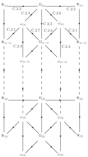
Figure 1: Steps necessary for completing the proof by induction

The following Subsections will verify the consistency of our central result (7.8) as well as (7.9), (7.10) with every single relation between various $\Omega_{(n)}$, $\omega_{(n)}$, $\bar{\omega}_{(n)}$, $\Psi_{(n)}$ due to the OPEs given in Section 2.

C.2.1 $\omega_{(n)},\bar{\omega}_{(n)}\rightarrow\Psi_{(n-1)}$ by $z_{A}\rightarrow z_{B}$ limit

Using the OPE (2.1d) one finds the following $z_{A}\rightarrow z_{B}$ behaviour for the $2n$ point correlators $\omega_{(n)}$:

$$\omega_{(n)}^{\mu_{1}...\mu_{2n-2}}\,{}_{\alpha}\,^{\beta}(z_{i})\Bigl{.}\Bigr{|}\begin{smallmatrix}z_{A}\\ \downarrow\\ z_{B}\end{smallmatrix}\ \ \sim\ \ \frac{-\,\delta_{\alpha}^{\beta}}{(z_{A}\,-\,z_{B})^{1/2}}\;\langle\psi^{\mu_{1}}(z_{1})\,...\,\psi^{\mu_{2n-2}}(z_{2n-2})\rangle\ \ =\ \ \frac{\delta_{\alpha}^{\beta}}{z_{AB}^{1/2}}\;\Psi^{\mu_{1}...\mu_{2n-2}}_{(n-1)}(z_{i})$$

$$=\ \ \frac{-\,\delta_{\alpha}^{\beta}}{z_{AB}^{1/2}}\!\sum_{\rho\in S_{2n-2}/{\cal Q}_{n,0}}\!\!\textrm{sgn}(\rho)\prod_{j=1}^{n-1}\frac{\eta^{\mu_{\rho(2j-1)}\mu_{\rho(2j)}}}{z_{\rho(2j-1)}\,-\,z_{\rho(2j)}}\,.$$ (C.4)

If we start from the expression (7.9) and isolate the highest $z_{AB}^{-1}$ powers, the sum over $\ell$ breaks down to the $\ell=0$ term where $\bigl{(}\sigma^{\mu_{\rho(1)}}...\bar{\sigma}^{\mu_{\rho(2\ell)}}\bigr{)}_{\alpha}\,^{\beta}\bigl{.}\bigr{|}_{\ell=0}=\delta^{\beta}_{\alpha}$:

$$\omega_{(n)}^{\mu_{1}...\mu_{2n-2}} \,{}_{\alpha}\,^{\beta}(z_{i})\Bigl{.}\Bigr{|}\begin{smallmatrix}z_{A}\\ \downarrow\\ z_{B}\end{smallmatrix}\ \ \sim\ \ \frac{-\,1}{z_{AB}^{1/2}}\;\prod_{i=1}^{2n-2}(z_{iA}\,z_{iB})^{-1/2}\,\sum_{\ell=0}^{n-1}\,\biggl{(}\frac{z_{AB}}{2}\biggr{)}^{\ell}\,\delta_{\ell,0}\!\!\!\!\sum_{\rho\in S_{2n-2}/{\cal Q}_{n,\ell}}\!\!\!\textrm{sgn}(\rho)$$

$$\ \ \ \ \ \ \ \times\,\bigl{(}\sigma^{\mu_{\rho(1)}}\,\bar{\sigma}^{\mu_{\rho(2)}}\,...\,\sigma^{\mu_{\rho(2\ell-1)}}\,\bar{\sigma}^{\mu_{\rho(2\ell)}}\bigr{)}_{\alpha}\,^{\beta}\,\prod_{j=1}^{n-\ell-1}\frac{\eta^{\mu_{\rho(2\ell+2j-1)}\mu_{\rho(2\ell+2j)}}}{z_{\rho(2\ell+2j-1),\rho(2\ell+2j)}}\;z_{\rho(2\ell+2j-1),A}\,z_{\rho(2\ell+2j),B}$$

$$=\ \ \frac{-\,\delta_{\alpha}^{\beta}}{z_{AB}^{1/2}}\!\sum_{\rho\in S_{2n-2}/{\cal Q}_{n,0}}\!\!\!\textrm{sgn}(\rho)\,\prod_{j=1}^{n-1}\frac{\eta^{\mu_{\rho(2j-1)}\mu_{\rho(2j)}}}{z_{\rho(2j-1),\rho(2j)}}\;\underbrace{\frac{z_{\rho(2j-1),A}\,z_{\rho(2j),B}}{\bigl{(}z_{\rho(2j-1),A}\,z_{\rho(2j-1),B}\,z_{\rho(2j),A}\,z_{\rho(2j),B}\bigr{)}^{1/2}}}_{\rightarrow 1\ \textrm{as}\ z_{A}\rightarrow z_{B}}$$

$$=\ \ \frac{-\,\delta_{\alpha}^{\beta}}{z_{AB}^{1/2}}\!\sum_{\rho\in S_{2n-2}/{\cal Q}_{n,0}}\!\!\textrm{sgn}(\rho)\prod_{j=1}^{n}\frac{\eta^{\mu_{\rho(2j-1)}\mu_{\rho(2j)}}}{z_{\rho(2j-1)}\,-\,z_{\rho(2j)}}\ .$$ (C.5)

Going to the third line we have rearranged the $\prod_{i=1}^{2n-2}(z_{iA}z_{iB})^{-1/2}$ product such that the cancellation with the $z_{\rho(2j-1),A}z_{\rho(2j),B}$ numerators in the $z_{A}\rightarrow z_{B}$ limit becomes obvious.

The argument for $\bar{\omega}_{(n)}$ is completely analogous. Due to the OPE (2.1e), one arrives at:

$$\bar{\omega}_{(n)}^{\mu_{1}...\mu_{2n-2}\dot{\alpha}}\,{}_{\dot{\beta}}(z_{i})\Bigl{.}\Bigr{|}\begin{smallmatrix}z_{A}\\ \downarrow\\ z_{B}\end{smallmatrix}\ \ \sim\ \ \frac{\delta^{\dot{\alpha}}_{\dot{\beta}}}{z_{AB}^{1/2}}\!\sum_{\rho\in S_{2n-2}/{\cal Q}_{n,0}}\!\!\textrm{sgn}(\rho)\prod_{j=1}^{n}\frac{\eta^{\mu_{\rho(2j-1)}\mu_{\rho(2j)}}}{z_{\rho(2j-1)}\,-\,z_{\rho(2j)}}\ .$$ (C.6)

This can also be obtained from (7.10) by virtue of the same truncation to the $\ell=0$ term and the identity $\prod_{j=1}^{n-1}\frac{z_{\rho(2j-1),A}z_{\rho(2j),B}}{(z_{\rho(2j-1),A}z_{\rho(2j-1),B}z_{\rho(2j),A}z_{\rho(2j),B})^{1/2}}\rightarrow 1$ used above. The agreement (C.4) $\leftrightarrow$ (C.5) in two ways of evaluating the $z_{A}\rightarrow z_{B}$ asymptotics, which extends to $\bar{\omega}_{(n)}$ by (C.6), allows to proceed to the next arrow in figure 1.

C.2.2 $\Omega_{(n)}\rightarrow\Psi_{(n)}$ by $z_{A}\rightarrow z_{B}$ limit

The relevant OPE for this case is (2.1b). Let us plug this into $\Omega_{(n)}$ for $z_{A}\rightarrow z_{B}$:

$$\Omega_{(n)} {}^{\mu_{1}...\mu_{2n-1}}\,_{\alpha\dot{\beta}}(z_{i})\Bigl{.}\Bigr{|}\begin{smallmatrix}z_{A}\\ \downarrow\\ z_{B}\end{smallmatrix}\ \ \sim\ \ \frac{1}{\sqrt{2}}\;(\sigma_{\mu_{2n}})_{\alpha\dot{\beta}}\,\langle\psi^{\mu_{1}}(z_{1})\,...\,\psi^{\mu_{2n-1}}(z_{2n-1})\,\psi^{\mu_{2n}}(z_{B})\rangle$$

$$=\ \ \frac{(\sigma_{\mu_{2n}})_{\alpha\dot{\beta}}}{\sqrt{2}}\;\Psi^{\mu_{1}...\mu_{2n}}_{(n)}(z_{i})\Bigl{.}\Bigr{|}_{z_{2n}=z_{B}}\ \ =\ \ \frac{(\sigma_{\mu_{2n}})_{\alpha\dot{\beta}}}{\sqrt{2}}\;\!\sum_{\rho\in S_{2n}/{\cal Q}_{n+1,0}}\!\!\textrm{sgn}(\rho)\prod_{j=1}^{n}\frac{\eta^{\mu_{\rho(2j-1)}\mu_{\rho(2j)}}}{z_{\rho(2j-1)}\,-\,z_{\rho(2j)}}\Bigl{.}\Bigr{|}_{z_{2n}=z_{B}}$$

$$=\ \ \frac{(\sigma_{\mu_{2n}})_{\alpha\dot{\beta}}}{\sqrt{2}}\;\!\sum_{\rho\in S_{2n}/{\cal Q}_{n+1,0}}\!\!\textrm{sgn}(\rho)\;\frac{\eta^{\mu_{\rho(2j_{0}-1)}\mu_{2n}}}{z_{\rho(2j_{0}-1)}\,-\,z_{B}}\;\prod_{j=1\atop{j\neq j_{0}\atop{\rho(2j_{0})=2n}}}^{n}\frac{\eta^{\mu_{\rho(2j-1)}\mu_{\rho(2j)}}}{z_{\rho(2j-1)}\,-\,z_{\rho(2j)}}$$

$$=\ \ \frac{1}{\sqrt{2}}\!\sum_{\rho\in S_{2n}/{\cal Q}_{n+1,0}}\!\!\textrm{sgn}(\rho)\;\frac{\sigma^{\mu_{\rho(2j_{0}-1)}}_{\alpha\dot{\beta}}}{z_{\rho(2j_{0}-1)}\,-\,z_{B}}\;\prod_{j=1\atop{j\neq j_{0}\atop{\rho(2j_{0})=2n}}}^{n}\frac{\eta^{\mu_{\rho(2j-1)}\mu_{\rho(2j)}}}{z_{\rho(2j-1)}\,-\,z_{\rho(2j)}}$$

$$=\ \ \frac{1}{\sqrt{2}}\!\sum_{\bar{\rho}\in S_{2n-1}/{\cal P}_{n,0}}\!\!\textrm{sgn}(\bar{\rho})\;\frac{\sigma^{\mu_{\bar{\rho}(1)}}_{\alpha\dot{\beta}}}{z_{\bar{\rho}(1)}\,-\,z_{B}}\;\prod_{j=1}^{n-1}\frac{\eta^{\mu_{\bar{\rho}(2j)}\mu_{\bar{\rho}(2j+1)}}}{z_{\bar{\rho}(2j)}\,-\,z_{\bar{\rho}(2j+1)}}\,.$$ (C.7)

Since the index $\mu_{2n}$ is contracted from the third to the fourth line, one can sum over $S_{2n-1}$ subpermutations $\bar{\rho}$ acting on $(1,2,...,2n-1)$ instead of $\rho\in S_{2n}$. The number of terms is the same in both sums,

$$\bigl{|}S_{2n}/{\cal Q}_{n+1,0}\bigr{|}\ \ =\ \ \frac{(2n)!}{n!\,2^{n}}\ \ =\ \ \frac{2n\,(2n\,-\,1)!}{n\,(n\,-\,1)!\,2\ 2^{n-1}}$$

$$=\ \ \frac{(2n\,-\,1)!}{(n\,-\,1)!\,2^{n-1}}\ \ =\ \ \bigl{|}S_{2n-1}/{\cal P}_{n,0}\bigr{|}\ ,$$ (C.8)

and one can check with the help of restrictions (7.11a), (7.11b) that the last equality of (C.7) holds exactly.

Can we reproduce (C.7) directly from $\Omega_{(n)}$ as claimed in (7.8) by keeping the most singular $z_{AB}$ dependences only? Similar to (C.5), the $\ell$ sum will reduce to the $\ell=0$ contribution:

$$\Omega_{(n)} {}^{\mu_{1}...\mu_{2n-1}}\,_{\alpha\dot{\beta}}(z_{i})\Bigl{.}\Bigr{|}\begin{smallmatrix}z_{A}\\ \downarrow\\ z_{B}\end{smallmatrix}\ \ \sim\ \ \frac{1}{\sqrt{2}}\prod_{i=1}^{2n-1}(z_{iA}\,z_{iB})^{-1/2}\,\sum_{\ell=0}^{n-1}\,\biggl{(}\frac{z_{AB}}{2}\biggr{)}^{\ell}\,\delta_{\ell,0}\!\!\!\!\sum_{\rho\in S_{2n-1}/{\cal P}_{n,\ell}}\!\!\!\textrm{sgn}(\rho)$$

$$\ \ \ \ \ \ \ \times\ \bigl{(}\sigma^{\mu_{\rho(1)}}\,\bar{\sigma}^{\mu_{\rho(2)}}\,...\,\bar{\sigma}^{\mu_{\rho(2\ell)}}\,\sigma^{\mu_{\rho(2\ell+1)}}\bigr{)}_{\alpha\dot{\beta}}\prod_{j=1}^{n-\ell-1}\frac{\eta^{\mu_{\rho(2\ell+2j)}\mu_{\rho(2\ell+2j+1)}}}{z_{\rho(2\ell+2j),\rho(2\ell+2j+1)}}\;z_{\rho(2\ell+2j),A}\,z_{\rho(2\ell+2j+1),B}$$

$$=\ \ \frac{1}{\sqrt{2}}\!\sum_{\rho\in S_{2n-1}/{\cal P}_{n,0}}\!\!\!\textrm{sgn}(\rho)\;\frac{1}{z_{\rho(1),A}^{1/2}\,z_{\rho(1),B}^{1/2}}\;\underbrace{\left(\frac{z_{\rho(1),A}}{z_{\rho(1),B}}\right)^{1/2}}_{\rightarrow 1\ \textrm{as}\ z_{A}\rightarrow z_{B}}\,\sigma^{\mu_{\rho(1)}}_{\alpha\dot{\beta}}$$

$$\ \ \ \ \ \ \ \times\ \prod_{j=1}^{n-1}\frac{\eta^{\mu_{\rho(2j)}\mu_{\rho(2j+1)}}}{z_{\rho(2j),\rho(2j+1)}}\;\underbrace{\frac{z_{\rho(2j),A}\,z_{\rho(2j+1),B}}{\bigl{(}z_{\rho(2j),A}\,z_{\rho(2j),B}\,z_{\rho(2j+1),A}\,z_{\rho(2j+1),B}\bigr{)}^{1/2}}}_{\rightarrow 1\ \textrm{as}\ z_{A}\rightarrow z_{B}}$$

$$=\ \ \frac{1}{\sqrt{2}}\!\sum_{\rho\in S_{2n-1}/{\cal P}_{n,0}}\!\!\!\textrm{sgn}(\rho)\;\frac{\sigma^{\mu_{\rho(1)}}_{\alpha\dot{\beta}}}{z_{\rho(1)}\,-\,z_{B}}\;\prod_{j=1}^{n-1}\frac{\eta^{\mu_{\rho(2j)}\mu_{\rho(2j+1)}}}{z_{\rho(2j)}\,-\,z_{\rho(2j+1)}}\,.$$ (C.9)

Except for the insertion of $\left(\frac{z_{\rho(1),A}}{z_{\rho(1),B}}\right)^{1/2}\rightarrow 1$, the mechanisms are the same as in (C.5).

C.2.3 $\Omega_{(n)}\rightarrow\Omega_{(n-1)}$ by $z_{2n-2}\rightarrow z_{2n-1}$ limit

This subsection treats the situation when the arguments of two NS field in $\Omega_{(n)}$ approach each other. We are left with the correlator $\Omega_{(n-1)}$ because of the OPE (2.1a):

$$\Omega_{(n)} {}^{\mu_{1}...\mu_{2n-1}}\,_{\alpha\dot{\beta}}(z_{i})\Bigl{.}\Bigr{|}\begin{smallmatrix}z_{2n-2}\\ \downarrow\\ z_{2n-1}\end{smallmatrix}\ \ \sim\ \ \frac{\eta^{\mu_{2n-2}\mu_{2n-1}}}{z_{2n-2}\,-\,z_{2n-1}}\;\langle\psi^{\mu_{1}}(z_{1})\,...\,\psi^{\mu_{2n-3}}(z_{2n-3})\,S_{\alpha}(z_{A})\,S_{\dot{\beta}}(z_{B})\rangle$$

$$=\ \ \frac{\eta^{\mu_{2n-2}\mu_{2n-1}}}{z_{2n-2}\,-\,z_{2n-1}}\;\Omega_{(n-1)}^{\mu_{1}...\mu_{2n-3}}\,{}_{\alpha\dot{\beta}}(z_{i})$$

$$=\ \ \frac{\eta^{\mu_{2n-2}\mu_{2n-1}}}{z_{2n-2,2n-1}}\;\frac{1}{\sqrt{2}}\prod_{i=1}^{2n-3}(z_{iA}\,z_{iB})^{-1/2}\,\sum_{\ell=0}^{n-2}\,\biggl{(}\frac{z_{AB}}{2}\biggr{)}^{\ell}\!\!\!\!\sum_{\rho\in S_{2n-3}/{\cal P}_{n-1,\ell}}\!\!\!\textrm{sgn}(\rho)\,\bigl{(}\sigma^{\mu_{\rho(1)}}\,...\,\sigma^{\mu_{\rho(2\ell+1)}}\bigr{)}_{\alpha\dot{\beta}}$$

$$\ \ \ \ \ \ \ \times\ \prod_{j=1}^{n-\ell-2}\frac{\eta^{\mu_{\rho(2\ell+2j)}\mu_{\rho(2\ell+2j+1)}}}{z_{\rho(2\ell+2j),\rho(2\ell+2j+1)}}\;z_{\rho(2\ell+2j),A}\,z_{\rho(2\ell+2j+1),B}\,.$$ (C.10)

To bring the asymptotic behaviour of expression (7.8) for $z_{2n-2}\rightarrow z_{2n-1}$ into the form (C.10) one has to isolate the permutations $S_{2n-1}/{\cal P}_{n,\ell}$ which provide a factor $\frac{\eta^{\mu_{2n-2}\mu_{2n-1}}}{z_{2n-2}-z_{2n-1}}$. A necessary condition for this to occur is $\ell\neq n-1$ because otherwise there would be no $\eta$’s at all. So we include $(1-\delta_{\ell,n-1})$.

Furthermore, the ordering of the $\eta$’s according to their second index (which is rephrased as $\rho(2\ell+3)<\rho(2\ell+5)<...<\rho(2n-1)$ in (7.11a)) makes sure that $\rho(2n-1)=2n-1$, and then $\eta^{\mu_{2n-2}\mu_{2n-1}}$ appears whenever $\rho(2n-2)=2n-2$. These arguments lead to

$$\Omega_{(n)} {}^{\mu_{1}...\mu_{2n-1}}\,_{\alpha\dot{\beta}}(z_{i})\Bigl{.}\Bigr{|}\begin{smallmatrix}z_{2n-2}\\ \downarrow\\ z_{2n-1}\end{smallmatrix}\ \ \sim\ \ \frac{1}{\sqrt{2}}\prod_{i=1}^{2n-1}(z_{iA}\,z_{iB})^{-1/2}\,\sum_{\ell=0}^{n-1}\,\biggl{(}\frac{z_{AB}}{2}\biggr{)}^{\ell}\,\bigl{(}1\,-\,\delta_{\ell,n-1}\bigr{)}\!\!\!\!\sum_{\rho\in S_{2n-1}/{\cal P}_{n,\ell}}\!\!\!\textrm{sgn}(\rho)$$

$$\ \ \ \ \ \ \ \times\ \delta_{\rho(2n-2),2n-2}\,\bigl{(}\sigma^{\mu_{\rho(1)}}\,...\,\sigma^{\mu_{\rho(2\ell+1)}}\bigr{)}_{\alpha\dot{\beta}}\,\prod_{j=1}^{n-\ell-1}\frac{\eta^{\mu_{\rho(2\ell+2j)}\mu_{\rho(2\ell+2j+1)}}}{z_{\rho(2\ell+2j),\rho(2\ell+2j+1)}}\;z_{\rho(2\ell+2j),A}\,z_{\rho(2\ell+2j+1),B}$$

$$=\ \ \frac{1}{\sqrt{2}}\prod_{i=1}^{2n-3}(z_{iA}\,z_{iB})^{-1/2}\,\sum_{\ell=0}^{n-2}\,\biggl{(}\frac{z_{AB}}{2}\biggr{)}^{\ell}\!\!\!\!\sum_{\rho\in S_{2n-1}/{\cal P}_{n,\ell}}\!\!\!\textrm{sgn}(\rho)\,\delta_{\rho(2n-2),2n-2}$$

$$\ \ \ \ \ \ \ \times\ \bigl{(}\sigma^{\mu_{\rho(1)}}\,...\,\sigma^{\mu_{\rho(2\ell+1)}}\bigr{)}_{\alpha\dot{\beta}}\;\frac{\eta^{\mu_{2n-2}\mu_{2n-1}}}{z_{2n-2,2n-1}}\;\underbrace{\frac{z_{2n-2,A}\,z_{2n-1,B}}{\bigl{(}z_{2n-2,A}\,z_{2n-2,B}\,z_{2n-1,A}\,z_{2n-1,B}\bigr{)}^{1/2}}}_{\rightarrow 1\ \textrm{as}\ z_{2n-2}\rightarrow z_{2n-1}}$$

$$\ \ \ \ \ \ \ \times\ \prod_{j=1}^{n-\ell-2}\frac{\eta^{\mu_{\rho(2\ell+2j)}\mu_{\rho(2\ell+2j+1)}}}{z_{\rho(2\ell+2j),\rho(2\ell+2j+1)}}\;z_{\rho(2\ell+2j),A}\,z_{\rho(2\ell+2j+1),B}$$

$$=\ \ \frac{1}{\sqrt{2}}\;\frac{\eta^{\mu_{2n-2}\mu_{2n-1}}}{z_{2n-2,2n-1}}\prod_{i=1}^{2n-3}(z_{iA}\,z_{iB})^{-1/2}\,\sum_{\ell=0}^{n-2}\,\biggl{(}\frac{z_{AB}}{2}\biggr{)}^{\ell}\!\!\!\!\sum_{\bar{\rho}\in S_{2n-3}/{\cal P}_{n-1,\ell}}\!\!\!\textrm{sgn}(\bar{\rho})$$

$$\ \ \ \ \ \ \ \times\ \bigl{(}\sigma^{\mu_{\bar{\rho}(1)}}\,...\,\sigma^{\mu_{\bar{\rho}(2\ell+1)}}\bigr{)}_{\alpha\dot{\beta}}\,\prod_{j=1}^{n-\ell-2}\frac{\eta^{\mu_{\bar{\rho}(2\ell+2j)}\mu_{\bar{\rho}(2\ell+2j+1)}}}{z_{\bar{\rho}(2\ell+2j),\bar{\rho}(2\ell+2j+1)}}\;z_{\bar{\rho}(2\ell+2j),A}\,z_{\bar{\rho}(2\ell+2j+1),B}\ .$$ (C.11)

In the last step we have used that $S_{2n-1}/{\cal P}_{n,\ell}$ with $\left(\begin{smallmatrix}\rho(2n-1)\\ \rho(2n-2)\end{smallmatrix}\right)=\left(\begin{smallmatrix}2n-1\\ 2n-2\end{smallmatrix}\right)$ is equivalent to $S_{2n-3}/{\cal P}_{n-1,\ell}$, where the subpermutation $\bar{\rho}\in S_{2n-3}$ is of the same sign as the corresponding $\rho\in S_{2n-1}$.

C.2.4 $\omega_{(n)},\bar{\omega}_{(n)}\rightarrow\omega_{(n-1)},\bar{\omega}_{(n-1)}$ by $z_{2n-3}\rightarrow z_{2n-2}$ limit

The singular behaviour of the $\omega_{(n)},\bar{\omega}_{(n)}$ in two NS arguments can be studied in a similar fashion:

$$\omega_{(n)} {}^{\mu_{1}...\mu_{2n-2}}\,_{\alpha}\,{}^{\beta}(z_{i})\Bigl{.}\Bigr{|}\begin{smallmatrix}z_{2n-3}\\ \downarrow\\ z_{2n-2}\end{smallmatrix}\ \ \sim\ \ \frac{\eta^{\mu_{2n-3}\mu_{2n-2}}}{z_{2n-3}\,-\,z_{2n-2}}\;\langle\psi^{\mu_{1}}(z_{1})\,...\,\psi^{\mu_{2n-4}}(z_{2n-4})\,S_{\alpha}(z_{A})\,S^{\beta}(z_{B})\rangle$$

$$=\ \ \frac{\eta^{\mu_{2n-3}\mu_{2n-2}}}{z_{2n-3}\,-\,z_{2n-2}}\;\omega_{(n-1)}^{\mu_{1}...\mu_{2n-4}}\,{}_{\alpha}\,^{\beta}(z_{i})$$

$$=\ \ -\,\frac{\eta^{\mu_{2n-3}\mu_{2n-2}}}{z_{2n-3,2n-2}}\;\left(\frac{1}{z_{AB}^{1/2}}\right)\prod_{i=1}^{2n-4}(z_{iA}\,z_{iB})^{-1/2}\,\sum_{\ell=0}^{n-2}\,\biggl{(}\frac{z_{AB}}{2}\biggr{)}^{\ell}\!\!\!\!\sum_{\rho\in S_{2n-4}/{\cal Q}_{n-1,\ell}}\!\!\!\textrm{sgn}(\rho)\,\bigl{(}\sigma^{\mu_{\rho(1)}}\,...\,\bar{\sigma}^{\mu_{\rho(2\ell)}}\bigr{)}_{\alpha}\,^{\beta}$$

$$\ \ \ \ \ \ \ \times\ \prod_{j=1}^{n-\ell-2}\frac{\eta^{\mu_{\rho(2\ell+2j-1)}\mu_{\rho(2\ell+2j)}}}{z_{\rho(2\ell+2j-1),\rho(2\ell+2j)}}\;z_{\rho(2\ell+2j-1),A}\,z_{\rho(2\ell+2j),B}\,.$$ (C.12)

When performing the limit $z_{2n-3}\rightarrow z_{2n-2}$ in (7.9) we have to focus on the terms with $\frac{\eta^{\mu_{2n-3}\mu_{2n-2}}}{z_{2n-3,2n-2}}$, i.e. firstly exclude $\ell=n-1$ (since this would distribute all ${}^{\mu_{i}}$ indices among the $\sigma$ matrices) and secondly find the appropriate $S_{2n-2}/{\cal Q}_{n,\ell}$ permutations which really attach $\mu_{2n-3}$ and $\mu_{2n-2}$ to the same Kronecker symbol. Equation (7.11b) requires $\rho(2\ell+2)<\rho(2\ell+4)<...<\rho(2n-2)$, so the projector to leading singular terms is simply $\delta_{\rho(2n-3),2n-3}$:

$$\omega_{(n)} {}^{\mu_{1}...\mu_{2n-2}}\,_{\alpha}\,{}^{\beta}(z_{i})\Bigl{.}\Bigr{|}\begin{smallmatrix}z_{2n-3}\\ \downarrow\\ z_{2n-2}\end{smallmatrix}\ \ \sim\ \ \frac{-\,1}{z_{AB}^{1/2}}\prod_{i=1}^{2n-2}(z_{iA}\,z_{iB})^{-1/2}\,\sum_{\ell=0}^{n-1}\,\biggl{(}\frac{z_{AB}}{2}\biggr{)}^{\ell}\,\bigl{(}1\,-\,\delta_{\ell,n-1}\bigr{)}\!\!\!\!\sum_{\rho\in S_{2n-2}/{\cal Q}_{n,\ell}}\!\!\!\textrm{sgn}(\rho)$$

$$\ \ \ \ \ \ \ \times\ \delta_{\rho(2n-3),2n-3}\,\bigl{(}\sigma^{\mu_{\rho(1)}}\,...\,\bar{\sigma}^{\mu_{\rho(2\ell)}}\bigr{)}_{\alpha}\,^{\beta}\,\prod_{j=1}^{n-\ell-1}\frac{\eta^{\mu_{\rho(2\ell+2j-1)}\mu_{\rho(2\ell+2j)}}}{z_{\rho(2\ell+2j-1),\rho(2\ell+2j)}}\;z_{\rho(2\ell+2j-1),A}\,z_{\rho(2\ell+2j),B}$$

$$=\ \ \frac{-\,1}{z_{AB}^{1/2}}\prod_{i=1}^{2n-4}(z_{iA}\,z_{iB})^{-1/2}\,\sum_{\ell=0}^{n-2}\,\biggl{(}\frac{z_{AB}}{2}\biggr{)}^{\ell}\!\!\!\!\sum_{\rho\in S_{2n-2}/{\cal Q}_{n,\ell}}\!\!\!\textrm{sgn}(\rho)\,\delta_{\rho(2n-3),2n-3}$$

$$\ \ \ \ \ \ \ \times\ \bigl{(}\sigma^{\mu_{\rho(1)}}\,...\,\bar{\sigma}^{\mu_{\rho(2\ell)}}\bigr{)}_{\alpha}\,^{\beta}\;\frac{\eta^{\mu_{2n-3}\mu_{2n-2}}}{z_{2n-3,2n-2}}\;\underbrace{\frac{z_{2n-3,A}\,z_{2n-2,B}}{\bigl{(}z_{2n-3,A}\,z_{2n-3,B}\,z_{2n-2,A}\,z_{2n-2,B}\bigr{)}^{1/2}}}_{\rightarrow 1\ \textrm{as}\ z_{2n-3}\rightarrow z_{2n-2}}$$

$$\ \ \ \ \ \ \ \times\ \prod_{j=1}^{n-\ell-2}\frac{\eta^{\mu_{\rho(2\ell+2j-1)}\mu_{\rho(2\ell+2j)}}}{z_{\rho(2\ell+2j-1),\rho(2\ell+2j)}}\;z_{\rho(2\ell+2j-1),A}\,z_{\rho(2\ell+2j),B}$$

$$=\ \ -\,\frac{\eta^{\mu_{2n-3}\mu_{2n-2}}}{z_{2n-3,2n-2}\,z_{AB}^{1/2}}\prod_{i=1}^{2n-4}(z_{iA}\,z_{iB})^{-1/2}\,\sum_{\ell=0}^{n-2}\,\biggl{(}\frac{z_{AB}}{2}\biggr{)}^{\ell}\!\!\!\!\sum_{\bar{\rho}\in S_{2n-4}/{\cal Q}_{n-1,\ell}}\!\!\!\textrm{sgn}(\bar{\rho})$$

$$\ \ \ \ \ \ \ \times\ \bigl{(}\sigma^{\mu_{\bar{\rho}(1)}}\,...\,\bar{\sigma}^{\mu_{\bar{\rho}(2\ell)}}\bigr{)}_{\alpha}\,^{\beta}\,\prod_{j=1}^{n-\ell-2}\frac{\eta^{\mu_{\bar{\rho}(2\ell+2j-1)}\mu_{\bar{\rho}(2\ell+2j)}}}{z_{\bar{\rho}(2\ell+2j-1),\bar{\rho}(2\ell+2j)}}\;z_{\bar{\rho}(2\ell+2j-1),A}\,z_{\bar{\rho}(2\ell+2j),B}\,.$$ (C.13)

Having read the arguments for $\Omega_{(n)}\rightarrow\Omega_{(n-1)}$ in Subsection C.2.3, the reader might not be surprised about $S_{2n-2}/{\cal Q}_{n,\ell}$ with $\rho(2n-3)=2n-3,\,\rho(2n-2)=2n-2$ being equivalent to $S_{2n-4}/{\cal Q}_{n-1,\ell}$.

This analysis is easily extended for $\bar{\omega}$, so the analogue of (C.12) and (C.13) will not be displayed explicitly.

C.2.5 $\Omega_{(n)}\rightarrow\omega_{(n)}$ by $z_{1}\rightarrow z_{B}$ limit

Let us now turn to a more sophisticated limiting process where a dotted spin field is converted into an undotted one via OPE (2.2b):

$$\Omega_{(n)} {}^{\mu_{1}...\mu_{2n-1}}\,_{\alpha\dot{\beta}}(z_{i})\Bigl{.}\Bigr{|}\begin{smallmatrix}z_{1}\\ \downarrow\\ z_{B}\end{smallmatrix}\ \ \sim\ \ \frac{i}{\sqrt{2}\,(z_{1}\,-\,z_{B})^{1/2}}\;(\sigma^{\mu_{1}})_{\gamma\dot{\beta}}\,\langle\psi^{\mu_{2}}(z_{2})\,...\,\psi^{\mu_{2n-1}}(z_{2n-1})\,S_{\alpha}(z_{A})\,S^{\gamma}(z_{B})\rangle$$

$$=\ \ \frac{i}{\sqrt{2}\,(z_{1}\,-\,z_{B})^{1/2}}\;\omega_{(n)}^{\mu_{2}...\mu_{2n-1}}\,{}_{\alpha}\,^{\gamma}(z_{i})\,(\sigma^{\mu_{1}})_{\gamma\dot{\beta}}$$

$$=\ \ \frac{1}{\sqrt{2}\,z_{1B}^{1/2}}\,\underbrace{\left(\frac{-\,i}{z_{AB}^{1/2}}\right)}_{\rightarrow\,z_{1A}^{-1/2}\ \textrm{as}\ z_{1}\rightarrow z_{B}}\,\prod_{i=2}^{2n-1}(z_{iA}\,z_{iB})^{-1/2}\,\sum_{\ell=0}^{n-1}\,\biggl{(}\frac{z_{AB}}{2}\biggr{)}^{\ell}\!\!\!\!\sum_{\rho\in S_{2n-2}/{\cal Q}_{n,\ell}}\!\!\!\textrm{sgn}(\rho)$$

$$\ \ \ \ \ \times\,\bigl{(}\sigma^{\mu_{\rho(2)}}\,...\,\bar{\sigma}^{\mu_{\rho(2\ell+1)}}\bigr{)}_{\alpha}\,^{\gamma}\,(\sigma^{\mu_{1}})_{\gamma\dot{\beta}}\prod_{j=1}^{n-\ell-1}\frac{\eta^{\mu_{\rho(2\ell+2j)}\mu_{\rho(2\ell+2j+1)}}}{z_{\rho(2\ell+2j),\rho(2\ell+2j+1)}}\;z_{\rho(2\ell+2j),A}\,z_{\rho(2\ell+2j+1),B}\,.$$ (C.14)

The factor $i$ originates from moving the field $\psi^{\mu_{1}}(z_{1})$ across $S_{\alpha}(z_{A})$ before applying the OPE of $\psi^{\mu_{1}}(z_{1})$ with $S_{\dot{\beta}}(z_{B})$. Using (B.2) our result (C.14) becomes:

$$\Omega_{(n)} {}^{\mu_{1}...\mu_{2n-1}}\,_{\alpha\dot{\beta}}(z_{i})\Bigl{.}\Bigr{|}\begin{smallmatrix}z_{1}\\ \downarrow\\ z_{B}\end{smallmatrix}\ \ \sim\ \ \frac{1}{\sqrt{2}\,(z_{1A}\,z_{1B})^{1/2}}\,\prod_{i=2}^{2n-1}(z_{iA}\,z_{iB})^{-1/2}\,\sum_{\ell=0}^{n-1}\,\biggl{(}\frac{z_{AB}}{2}\biggr{)}^{\ell}\!\!\!\!\sum_{\rho\in S_{2n-2}/{\cal Q}_{n,\ell}}\!\!\!\textrm{sgn}(\rho)$$

$$\ \ \ \ \ \ \ \times\,\biggl{\{}\bigl{(}\sigma^{\mu_{1}}\,\bar{\sigma}^{\mu_{\rho(2)}}\,...\,\sigma^{\mu_{\rho(2\ell+1)}}\bigr{)}_{\alpha\dot{\beta}}\biggr{.}$$

$$\ \ \ \ \ \ \ \ \ \ -\ \underline{2}\,\sum_{k=1}^{\ell}\eta^{\mu_{1}\mu_{\rho(2k+1)}}\;\underbrace{\frac{z_{1A}\,z_{\rho(2k+1),B}}{\underline{z_{AB}}\,z_{1,\rho(2k+1)}}}_{\rightarrow 1\ \textrm{as}\ z_{1}\rightarrow z_{B}}\;\bigl{(}\sigma^{\mu_{\rho(2)}}\,...\,\sigma^{\mu_{\rho(2k)}}\,\bar{\sigma}^{\mu_{\rho(2k+2)}}\,...\,\sigma^{\mu_{\rho(2\ell+1)}}\bigr{)}_{\alpha\dot{\beta}}\biggr{.}$$

$$\ \ \ \ \ \ \ \ \ \ \ \biggl{.}+\ \underline{2}\,\sum_{k=1}^{\ell}\eta^{\mu_{1}\mu_{\rho(2k)}}\;\underbrace{\frac{z_{1A}\,z_{\rho(2k),B}}{\underline{z_{AB}}\,z_{1,\rho(2k)}}}_{\rightarrow 1\ \textrm{as}\ z_{1}\rightarrow z_{B}}\;\bigl{(}\sigma^{\mu_{\rho(2)}}\,...\,\bar{\sigma}^{\mu_{\rho(2k-1)}}\,\sigma^{\mu_{\rho(2k+1)}}\,...\,\sigma^{\mu_{\rho(2\ell+1)}}\bigr{)}_{\alpha\dot{\beta}}\biggr{\}}$$

$$\ \ \ \ \ \ \ \times\,\prod_{j=1}^{n-\ell-1}\frac{\eta^{\mu_{\rho(2\ell+2j)}\mu_{\rho(2\ell+2j+1)}}}{z_{\rho(2\ell+2j),\rho(2\ell+2j+1)}}\;z_{\rho(2\ell+2j),A}\,z_{\rho(2\ell+2j+1),B}$$

$$=\ \ \frac{1}{\sqrt{2}}\,\prod_{i=1}^{2n-1}(z_{iA}\,z_{iB})^{-1/2}\,\sum_{\ell^{\prime}=0}^{n-1}\,\biggl{(}\frac{z_{AB}}{2}\biggr{)}^{\ell^{\prime}}\,\Biggl{\{}\sum_{\rho\in S_{2n-2}/{\cal Q}_{n,\ell^{\prime}}}\!\!\!\textrm{sgn}(\rho)\Biggr{.}$$

$$\ \ \ \ \ \ \ \ \ \ \times\ \Biggl{.}\bigl{(}\sigma^{\mu_{1}}\,\bar{\sigma}^{\mu_{\rho(2)}}\,...\,\sigma^{\mu_{\rho(2\ell^{\prime}+1)}}\bigr{)}_{\alpha\dot{\beta}}\,\prod_{j=1}^{n-\ell^{\prime}-1}\frac{\eta^{\mu_{\rho(2\ell^{\prime}+2j)}\mu_{\rho(2\ell^{\prime}+2j+1)}}}{z_{\rho(2\ell^{\prime}+2j),\rho(2\ell^{\prime}+2j+1)}}\;z_{\rho(2\ell^{\prime}+2j),A}\,z_{\rho(2\ell^{\prime}+2j+1),B}$$

$$\ \ \ \ \ +\ \!\!\!\!\!\!\!\!\sum_{\rho\in S_{2n-2}/{\cal Q}_{n,\ell^{\prime}+1}}\!\!\!\!\!\!\!\bigl{(}+\textrm{sgn}(\rho)\bigr{)}\,\sum_{k=1}^{\ell^{\prime}+1}\bigl{(}\sigma^{\mu_{\rho(2)}}\,...\,\bar{\sigma}^{\mu_{\rho(2k-1)}}\,\sigma^{\mu_{\rho(2k+1)}}\,...\,\sigma^{\mu_{\rho(2\ell^{\prime}+3)}}\bigr{)}_{\alpha\dot{\beta}}\;\frac{\eta^{\mu_{1}\mu_{\rho(2k)}}}{z_{1,\rho(2k)}}\;z_{1A}\,z_{\rho(2k),B}$$

$$\ \ \ \ \ \ \ \ \ \ \times\,\prod_{j=1}^{n-\ell^{\prime}-2}\frac{\eta^{\mu_{\rho(2\ell^{\prime}+2j+2)}\mu_{\rho(2\ell^{\prime}+2j+3)}}}{z_{\rho(2\ell^{\prime}+2j+2),\rho(2\ell^{\prime}+2j+3)}}\;z_{\rho(2\ell^{\prime}+2j+2),A}\,z_{\rho(2\ell^{\prime}+2j+3),B}$$

$$\ \ \ \ \ \ \Biggl{.}+\ \!\!\!\!\!\!\!\!\sum_{\rho\in S_{2n-2}/{\cal Q}_{n,\ell^{\prime}+1}}\!\!\!\!\!\!\!\bigl{(}-\textrm{sgn}(\rho)\bigr{)}\,\sum_{k=1}^{\ell^{\prime}+1}\bigl{(}\sigma^{\mu_{\rho(2)}}\,...\,\sigma^{\mu_{\rho(2k)}}\,\bar{\sigma}^{\mu_{\rho(2k+2)}}\,...\,\sigma^{\mu_{\rho(2\ell^{\prime}+3)}}\bigr{)}_{\alpha\dot{\beta}}\;\frac{\eta^{\mu_{1}\mu_{\rho(2k+1)}}}{z_{1,\rho(2k+1)}}\;z_{1A}\,z_{\rho(2k+1),B}$$

$$\ \ \ \ \ \ \ \ \ \ \times\,\prod_{j=1}^{n-\ell^{\prime}-2}\frac{\eta^{\mu_{\rho(2\ell^{\prime}+2j+2)}\mu_{\rho(2\ell^{\prime}+2j+3)}}}{z_{\rho(2\ell^{\prime}+2j+2),\rho(2\ell^{\prime}+2j+3)}}\;z_{\rho(2\ell^{\prime}+2j+2),A}\,z_{\rho(2\ell^{\prime}+2j+3),B}\Biggr{\}}$$

$$=\ \ \frac{1}{\sqrt{2}}\,\prod_{i=1}^{2n-1}(z_{iA}\,z_{iB})^{-1/2}\,\sum_{\ell^{\prime}=0}^{n-1}\,\biggl{(}\frac{z_{AB}}{2}\biggr{)}^{\ell^{\prime}}\!\!\!\!\sum_{\bar{\rho}\in S_{2n-1}/{\cal P}_{n,\ell^{\prime}}}\!\!\!\textrm{sgn}(\bar{\rho})$$

$$\ \ \ \ \ \ \ \times\,\bigl{(}\sigma^{\mu_{\bar{\rho}(1)}}\,...\,\sigma^{\mu_{\bar{\rho}(2\ell^{\prime}+1)}}\bigr{)}_{\alpha\dot{\beta}}\,\prod_{j=0}^{n-\ell^{\prime}-2}\frac{\eta^{\mu_{\bar{\rho}(2\ell^{\prime}+2j+2)}\mu_{\bar{\rho}(2\ell^{\prime}+2j+3)}}}{z_{\bar{\rho}(2\ell^{\prime}+2j+2),\bar{\rho}(2\ell^{\prime}+2j+3)}}\;z_{\bar{\rho}(2\ell^{\prime}+2j+2),A}\,z_{\bar{\rho}(2\ell^{\prime}+2j+3),B}\ .$$ (C.15)

Several steps might require some further explanation here: Firstly, in oder to see that the inserted terms $\frac{z_{1A}z_{\rho(2k+1),B}}{z_{AB}z_{1,\rho(2k+1)}}$ and $\frac{z_{1A}z_{\rho(2k),B}}{z_{AB}z_{1,\rho(2k)}}$ really tend to 1 in the limit $z_{1}\rightarrow z_{B}$, one has to apply the crossing identity (2.10) to the numerators, i.e. $z_{1A}z_{\rho(2k),B}=z_{1B}z_{\rho(2k),A}+z_{1,\rho(2k)}z_{AB}$. Secondly, the underlined factors $\frac{2}{z_{AB}}$ in the third and fourth line shift the summation variable $\ell$ by 1. Thirdly, we have replaced one $S_{2n-2}/{\cal Q}_{n,\ell^{\prime}}$ sum and $2\ell^{\prime}+2$ sums over $S_{2n-2}/{\cal Q}_{n,\ell^{\prime}+1}$ by the $S_{2n-1}/{\cal P}_{n,\ell^{\prime}}$ sum over larger permutations $\bar{\rho}$ including $\mu_{1}$. The total number of terms is the same since:

$$\bigl{|}S_{2n-2}/{\cal Q}_{n,\ell} \bigr{|}\ +\ (2\ell\,+\,2)\,\bigl{|}S_{2n-2}/{\cal Q}_{n,\ell+1}\bigr{|}\ \ =\ \ \frac{(2n\,-\,2)!}{(2\ell)!\,(n\,-\,\ell\,-\,1)!\,2^{n-\ell-1}}$$

$$\ \ \ \ \ \ +\ \frac{(2\ell\,+\,2)\,(2n\,-\,2)!}{(2\ell\,+\,2)!\,(n\,-\,\ell\,-\,2)!\,2^{n-\ell-2}}$$

$$=\ \ \frac{(2n\,-\,2)!}{(2\ell\,+\,1)!\,(n\,-\,\ell\,-\,1)!\,2^{n-\ell-1}}\;\Bigl{(}2\ell\,+\,1\,+\,2\ (n-\ell-1)\Bigr{)}$$

$$=\ \ \frac{(2n\,-\,1)!}{(2\ell\,+\,1)!\,(n\,-\,\ell\,-\,1)!\,2^{n-\ell-1}}$$

$$=\ \ \bigl{|}S_{2n-1}/{\cal P}_{n,\ell}\bigr{|}\ .$$ (C.16)

Moreover, the index $\mu_{1}$ appears in all possible positions in (C.15), i.e. attached to $\sigma$’s as well as to $\eta$’s. The relative sign between $\rho$ and $\bar{\rho}$ is taken into account.

Following the general principle of this proof, we should now compare the final line of (C.15) with the most singular terms in the expression (7.8) for $\Omega_{(n)}$. Due to our particular arrangement of $\sigma$ matrices $\rho(1)<...<\rho(2\ell+1)$, no factors of $z_{1}-z_{B}$ appear in any denominator. So equation (7.8) does not simplify in the $z_{1}\rightarrow z_{B}$ regime. However, it already matches with (C.15) up to a shift in the $j$ product, so we are done with the $\Omega_{(n)}\rightarrow\omega_{(n)}$ reduction.

Actually, this is the reason we sent $z_{1}$ and not any other $z_{i}$, $i=2,3,...,2n-1$, to $z_{B}$. the more $z_{ij}$ dependences of different index structures are successfully reproduced, the more convincing becomes this part of the proof.

C.2.6 $\Omega_{(n)}\rightarrow\bar{\omega}_{(n)}$ by $z_{2n-1}\rightarrow z_{A}$ limit

The “dotted” analogue of the preceding limit requires the use of the OPE (2.2a). For reasons given in the end of the previous subsections the behaviour for $z_{2n-1}\rightarrow z_{A}$ gives rise to the richest consistency checks as the right hand side of (7.8) does not have any poles in $(z_{2n-1}-z_{A})$. In detail, the limiting behaviour is given by:

$$\Omega {}_{(n)}^{\mu_{1}...\mu_{2n-1}}\,{}_{\alpha\dot{\beta}}(z_{i})\Bigl{.}\Bigr{|}\begin{smallmatrix}z_{2n-1}\\ \downarrow\\ z_{A}\end{smallmatrix}\ \ \sim\ \ \frac{(\sigma^{\mu_{2n-1}})_{\alpha\dot{\gamma}}}{\sqrt{2}\,(z_{2n-1}\,-\,z_{A})^{1/2}}\;\langle\psi^{\mu_{1}}(z_{1})\,...\,\psi^{\mu_{2n-2}}(z_{2n-2})\,S^{\dot{\gamma}}(z_{A})\,S_{\dot{\beta}}(z_{B})\rangle$$

$$=\ \ \frac{1}{\sqrt{2}\,(z_{2n-1}\,-\,z_{A})^{1/2}}\;(\sigma^{\mu_{2n-1}})_{\alpha\dot{\gamma}}\,\bar{\omega}_{(n)}^{\mu_{1}...\mu_{2n-2}\dot{\gamma}}\,{}_{\dot{\beta}}(z_{i})$$

$$=\ \ \frac{1}{\sqrt{2}\,z_{2n-1,A}^{1/2}}\,\underbrace{\left(\frac{1}{z_{AB}^{1/2}}\right)}_{\rightarrow\,z_{2n-1,B}^{-1/2}\ \textrm{as}\ z_{2n-1}\rightarrow z_{A}}\,\prod_{i=1}^{2n-2}(z_{iA}\,z_{iB})^{-1/2}\,\sum_{\ell=0}^{n-1}\,\biggl{(}\frac{z_{AB}}{2}\biggr{)}^{\ell}\!\!\!\!\sum_{\rho\in S_{2n-2}/{\cal Q}_{n,\ell}}\!\!\!\textrm{sgn}(\rho)$$

$$\ \ \ \ \ \ \ \times\,(\sigma^{\mu_{2n-1}})_{\alpha\dot{\gamma}}\,\bigl{(}\bar{\sigma}^{\mu_{\rho(1)}}\,...\,\sigma^{\mu_{\rho(2\ell)}}\bigr{)}^{\dot{\gamma}}\,_{\dot{\beta}}\,\prod_{j=1}^{n-\ell-1}\frac{\eta^{\mu_{\rho(2\ell+2j-1)}\mu_{\rho(2\ell+2j)}}}{z_{\rho(2\ell+2j-1),\rho(2\ell+2j)}}\;z_{\rho(2\ell+2j-1),A}\,z_{\rho(2\ell+2j),B}\ .$$ (C.17)

At this point we use the identity (B.2):

$$\Omega {}_{(n)}^{\mu_{1}...\mu_{2n-1}}\,{}_{\alpha\dot{\beta}}(z_{i})\Bigl{.}\Bigr{|}\begin{smallmatrix}z_{2n-1}\\ \downarrow\\ z_{A}\end{smallmatrix}\ \ \sim\ \ \frac{1}{\sqrt{2}}\,\prod_{i=1}^{2n-1}(z_{iA}\,z_{iB})^{-1/2}\,\sum_{\ell=0}^{n-1}\,\biggl{(}\frac{z_{AB}}{2}\biggr{)}^{\ell}\!\!\!\!\sum_{\rho\in S_{2n-2}/{\cal Q}_{n,\ell}}\!\!\!\textrm{sgn}(\rho)$$

$$\ \ \ \ \ \ \ \times\,\biggl{\{}\bigl{(}\sigma^{\mu_{\rho(1)}}\,...\,\bar{\sigma}^{\mu_{\rho(2\ell)}}\,\sigma^{\mu_{2n-1}}\bigr{)}_{\alpha\dot{\beta}}\biggr{.}$$

$$\ \ \ \ \ \ \ \ \ \ -\ \underline{2}\,\sum_{k=1}^{\ell}\eta^{\mu_{\rho(2k-1)}\mu_{2n-1}}\;\underbrace{\frac{z_{\rho(2k-1),A}\,z_{2n-1,B}}{\underline{z_{AB}}\,z_{2n-1,\rho(2k-1)}}}_{\rightarrow 1\ \textrm{as}\ z_{2n-1}\rightarrow z_{A}}\;\bigl{(}\sigma^{\mu_{\rho(1)}}\,...\,\bar{\sigma}^{\mu_{\rho(2k-2)}}\,\sigma^{\mu_{\rho(2k)}}\,...\,\sigma^{\mu_{\rho(2\ell)}}\bigr{)}_{\alpha\dot{\beta}}\biggr{.}$$

$$\ \ \ \ \ \ \ \ \ \ \ \biggl{.}+\ \underline{2}\,\sum_{k=1}^{\ell}\eta^{\mu_{\rho(2k)}\mu_{2n-1}}\;\underbrace{\frac{z_{\rho(2k),A}\,z_{2n-1,B}}{\underline{z_{AB}}\,z_{\rho(2k),2n-1}}}_{\rightarrow 1\ \textrm{as}\ z_{2n-1}\rightarrow z_{A}}\;\bigl{(}\sigma^{\mu_{\rho(1)}}\,...\,\sigma^{\mu_{\rho(2k-1)}}\,\bar{\sigma}^{\mu_{\rho(2k+1)}}\,...\,\sigma^{\mu_{\rho(2\ell)}}\bigr{)}_{\alpha\dot{\beta}}\biggr{\}}$$

$$\ \ \ \ \ \ \ \times\,\prod_{j=1}^{n-\ell-1}\frac{\eta^{\mu_{\rho(2\ell+2j-1)}\mu_{\rho(2\ell+2j)}}}{z_{\rho(2\ell+2j-1),\rho(2\ell+2j)}}\;z_{\rho(2\ell+2j-1),A}\,z_{\rho(2\ell+2j),B}$$

$$=\ \ \frac{1}{\sqrt{2}}\,\prod_{i=1}^{2n-1}(z_{iA}\,z_{iB})^{-1/2}\,\sum_{\ell^{\prime}=0}^{n-1}\,\biggl{(}\frac{z_{AB}}{2}\biggr{)}^{\ell^{\prime}}\,\Biggl{\{}\sum_{\rho\in S_{2n-2}/{\cal Q}_{n,\ell^{\prime}}}\!\!\!\textrm{sgn}(\rho)\Biggr{.}$$

$$\ \ \ \ \ \ \ \ \ \ \times\ \Biggl{.}\bigl{(}\sigma^{\mu_{\rho(1)}}\,...\,\bar{\sigma}^{\mu_{\rho(2\ell^{\prime})}}\,\sigma^{\mu_{2n-1}}\bigr{)}_{\alpha\dot{\beta}}\,\prod_{j=1}^{n-\ell^{\prime}-1}\frac{\eta^{\mu_{\rho(2\ell^{\prime}+2j-1)}\mu_{\rho(2\ell^{\prime}+2j)}}}{z_{\rho(2\ell^{\prime}+2j-1),\rho(2\ell^{\prime}+2j)}}\;z_{\rho(2\ell^{\prime}+2j-1),A}\,z_{\rho(2\ell^{\prime}+2j),B}$$

$$\ \ \ \ \ +\ \!\!\!\!\!\!\!\sum_{\rho\in S_{2n-2}/{\cal Q}_{n,\ell^{\prime}+1}}\!\!\!\!\!\!\!\bigl{(}+\textrm{sgn}(\rho)\bigr{)}\,\sum_{k=1}^{\ell^{\prime}+1}\bigl{(}\sigma^{\mu_{\rho(1)}}\,...\,\sigma^{\mu_{\rho(2k-1)}}\,\bar{\sigma}^{\mu_{\rho(2k+1)}}\,...\sigma^{\mu_{\rho(2\ell^{\prime}+2)}}\bigr{)}_{\alpha\dot{\beta}}\;\frac{\eta^{\mu_{\rho(2k)}\mu_{2n-1}}}{z_{\rho(2k),2n-1}}$$

$$\ \ \ \ \ \ \ \ \ \ \times\,z_{\rho(2k),A}\,z_{2n-1,B}\,\prod_{j=1}^{n-\ell^{\prime}-2}\frac{\eta^{\mu_{\rho(2\ell^{\prime}+2j+1)}\mu_{\rho(2\ell^{\prime}+2j+2)}}}{z_{\rho(2\ell^{\prime}+2j+1),\rho(2\ell^{\prime}+2j+2)}}\;z_{\rho(2\ell^{\prime}+2j+1),A}\,z_{\rho(2\ell^{\prime}+2j+2),B}$$

$$\ \ \ \ \ \ \Biggl{.}+\ \!\!\!\!\!\!\!\sum_{\rho\in S_{2n-2}/{\cal Q}_{n,\ell^{\prime}+1}}\!\!\!\!\!\!\!\bigl{(}-\textrm{sgn}(\rho)\bigr{)}\,\sum_{k=1}^{\ell^{\prime}+1}\bigl{(}\sigma^{\mu_{\rho(1)}}\,...\,\bar{\sigma}^{\mu_{\rho(2k-2)}}\,\sigma^{\mu_{\rho(2k)}}\,...\,\sigma^{\mu_{\rho(2\ell^{\prime}+2)}}\bigr{)}_{\alpha\dot{\beta}}\;\frac{\eta^{\mu_{\rho(2k-1)}\mu_{2n-1}}}{z_{\rho(2k-1),2n-1}}$$

$$\ \ \ \ \ \ \ \ \ \ \times\,z_{\rho(2k-1),A}\,z_{2n-1,B}\,\prod_{j=1}^{n-\ell^{\prime}-2}\frac{\eta^{\mu_{\rho(2\ell^{\prime}+2j+1)}\mu_{\rho(2\ell^{\prime}+2j+2)}}}{z_{\rho(2\ell^{\prime}+2j+1),\rho(2\ell^{\prime}+2j+2)}}\;z_{\rho(2\ell^{\prime}+2j+1),A}\,z_{\rho(2\ell^{\prime}+2j+2),B}\Biggr{\}}$$

$$=\ \ \frac{1}{\sqrt{2}}\,\prod_{i=1}^{2n-1}(z_{iA}\,z_{iB})^{-1/2}\,\sum_{\ell^{\prime}=0}^{n-1}\,\biggl{(}\frac{z_{AB}}{2}\biggr{)}^{\ell^{\prime}}\!\!\!\!\sum_{\bar{\rho}\in S_{2n-1}/{\cal P}_{n,\ell^{\prime}}}\!\!\!\textrm{sgn}(\bar{\rho})$$

$$\ \ \ \ \ \ \ \times\,\bigl{(}\sigma^{\mu_{\bar{\rho}(1)}}\,...\,\sigma^{\mu_{\bar{\rho}(2\ell^{\prime}+1)}}\bigr{)}_{\alpha\dot{\beta}}\,\prod_{j=0}^{n-\ell^{\prime}-2}\frac{\eta^{\mu_{\bar{\rho}(2\ell^{\prime}+2j+2)}\mu_{\bar{\rho}(2\ell^{\prime}+2j+3)}}}{z_{\bar{\rho}(2\ell^{\prime}+2j+2),\bar{\rho}(2\ell^{\prime}+2j+3)}}\;z_{\bar{\rho}(2\ell^{\prime}+2j+2),A}\,z_{\bar{\rho}(2\ell^{\prime}+2j+3),B}\,.$$ (C.18)

This is the exact expression for $\Omega_{(n)}$. So we can move on to the next case $\omega_{(n)}\rightarrow\Omega_{(n-1)}$.

C.2.7 $\omega_{(n)}\rightarrow\Omega_{(n-1)}$ by $z_{1}\rightarrow z_{B}$ limit

The reduction of $\omega_{(n)}$ to correlators of $\Omega_{(n-1)}$ type is based on the OPE (2.2a):

$$\omega {}_{(n)}^{\mu_{1}...\mu_{2n-2}}\,{}_{\alpha}\,^{\beta}(z_{i})\Bigl{.}\Bigr{|}\begin{smallmatrix}z_{1}\\ \downarrow\\ z_{B}\end{smallmatrix}\ \ \sim\ \ \frac{i}{\sqrt{2}\,(z_{1}\,-\,z_{B})^{1/2}}\;(\bar{\sigma}^{\mu_{1}})^{\dot{\gamma}\beta}\,\langle\psi^{\mu_{2}}(z_{2})\,...\,\psi^{\mu_{2n-2}}(z_{2n-2})\,S_{\alpha}(z_{A})\,S_{\dot{\gamma}}(z_{B})\rangle$$

$$=\ \ \frac{i}{\sqrt{2}\,(z_{1}\,-\,z_{B})^{1/2}}\;\Omega_{(n-1)}^{\mu_{2}...\mu_{2n-2}}\,{}_{\alpha\dot{\gamma}}(z_{i})\,(\bar{\sigma}^{\mu_{1}})^{\dot{\gamma}\beta}$$

$$=\ \ \frac{i}{2\,z_{1B}^{1/2}}\;\underbrace{\frac{z_{AB}}{z_{AB}^{1/2}\,z_{1A}^{1/2}}}_{\rightarrow\,-i\ \textrm{as}\ z_{1}\rightarrow z_{B}}\,\prod_{i=2}^{2n-2}(z_{iA}\,z_{iB})^{-1/2}\,\sum_{\ell=0}^{n-2}\,\biggl{(}\frac{z_{AB}}{2}\biggr{)}^{\ell}\!\!\!\!\!\sum_{\rho\in S_{2n-3}/{\cal P}_{n-1,\ell}}\!\!\!\!\textrm{sgn}(\rho)$$

$$\ \ \ \ \ \times\,\bigl{(}\sigma^{\mu_{\rho(2)}}\,...\,\sigma^{\mu_{\rho(2\ell+2)}}\bigr{)}_{\alpha\dot{\gamma}}\,(\bar{\sigma}^{\mu_{1}})^{\dot{\gamma}\beta}\!\prod_{j=1}^{n-\ell-2}\frac{\eta^{\mu_{\rho(2\ell+2j+1)}\mu_{\rho(2\ell+2j+2)}}}{z_{\rho(2\ell+2j+1),\rho(2\ell+2j+2)}}\;z_{\rho(2\ell+2j+1),A}\,z_{\rho(2\ell+2j+2),B}\,.$$ (C.19)

Here, it is necessary to move the $\bar{\sigma}^{\mu_{1}}$ to the left of $\sigma^{\mu_{\rho(2)}}...\sigma^{\mu_{\rho(2\ell+2)}}$, i.e. across an odd number of $\sigma$ matrices. With the help of (B.3) we obtain:

$$\omega_{(n)} {}^{\mu_{1}...\mu_{2n-2}}\,_{\alpha}\,{}^{\beta}(z_{i})\Bigl{.}\Bigr{|}\begin{smallmatrix}z_{1}\\ \downarrow\\ z_{B}\end{smallmatrix}\ \ \sim\ \ \frac{\underline{z_{AB}}}{\underline{2}\,z_{AB}^{1/2}\,z_{1A}^{1/2}\,z_{1B}^{1/2}}\;\prod_{i=2}^{2n-2}(z_{iA}\,z_{iB})^{-1/2}\,\sum_{\ell=0}^{n-2}\,\biggl{(}\frac{z_{AB}}{2}\biggr{)}^{\ell}$$

$$\ \ \ \ \ \ \ \times\!\!\!\!\sum_{\rho\in S_{2n-3}/{\cal P}_{n-1,\ell}}\!\!\!\!\!\textrm{sgn}(\rho)\,\Biggl{\{}-\ \bigl{(}\sigma^{\mu_{1}}\,\bar{\sigma}^{\mu_{\rho(2)}}\,...\,\bar{\sigma}^{\mu_{\rho(2\ell+2)}}\bigr{)}_{\alpha}\,^{\beta}\,\Biggr{.}$$

$$\ \ \ \ \ \ \ \ \ \ -\ \underline{2}\,\sum_{k=1}^{\ell+1}\eta^{\mu_{1}\mu_{\rho(2k)}}\;\underbrace{\frac{z_{1A}\,z_{\rho(2k),B}}{z_{1,\rho(2k)}\,\underline{z_{AB}}}}_{\rightarrow 1\ \textrm{as}\ z_{1}\rightarrow z_{B}}\;\bigl{(}\sigma^{\mu_{\rho(2)}}\,...\,\bar{\sigma}^{\mu_{\rho(2k-1)}}\,\sigma^{\mu_{\rho(2k+1)}}\,...\,\bar{\sigma}^{\mu_{\rho(2\ell+2)}}\bigr{)}_{\alpha}\,^{\beta}$$

$$\ \ \ \ \ \ \ \ \ \ \ \Biggl{.}+\ \underline{2}\,\sum_{k=1}^{\ell}\eta^{\mu_{1}\mu_{\rho(2k+1)}}\;\underbrace{\frac{z_{1A}\,z_{\rho(2k+1),B}}{z_{1,\rho(2k+1)}\,\underline{z_{AB}}}}_{\rightarrow 1\ \textrm{as}\ z_{1}\rightarrow z_{B}}\;\bigl{(}\sigma^{\mu_{\rho(2)}}\,...\,\sigma^{\mu_{\rho(2k)}}\,\bar{\sigma}^{\mu_{\rho(2k+2)}}\,...\,\bar{\sigma}^{\mu_{\rho(2\ell+2)}}\bigr{)}_{\alpha}\,^{\beta}\Biggr{\}}$$

$$\ \ \ \ \ \ \ \times\,\prod_{j=1}^{n-\ell-2}\frac{\eta^{\mu_{\rho(2\ell+2j+1)}\mu_{\rho(2\ell+2j+2)}}}{z_{\rho(2\ell+2j+1),\rho(2\ell+2j+2)}}\;z_{\rho(2\ell+2j+1),A}\,z_{\rho(2\ell+2j+2),B}$$

$$=\ \ \frac{-\,1}{z_{AB}^{1/2}}\,\prod_{i=1}^{2n-2}(z_{iA}\,z_{iB})^{-1/2}\,\sum_{\ell^{\prime}=0}^{n-1}\,\biggl{(}\frac{z_{AB}}{2}\biggr{)}^{\ell^{\prime}}\Biggl{\{}\sum_{\rho\in S_{2n-3}/{\cal P}_{n-1,\ell^{\prime}-1}}\!\!\!\!\!\textrm{sgn}(\rho)\Biggr{.}$$

$$\ \ \ \ \ \ \ \times\,\bigl{(}\sigma^{\mu_{1}}\,\bar{\sigma}^{\mu_{\rho(2)}}\,...\,\bar{\sigma}^{\mu_{\rho(2\ell^{\prime})}}\bigr{)}_{\alpha}\,^{\beta}\,\prod_{j=1}^{n-\ell^{\prime}-1}\frac{\eta^{\mu_{\rho(2\ell^{\prime}+2j-1)}\mu_{\rho(2\ell^{\prime}+2j)}}}{z_{\rho(2\ell^{\prime}+2j-1),\rho(2\ell^{\prime}+2j)}}\;z_{\rho(2\ell^{\prime}+2j-1),A}\,z_{\rho(2\ell^{\prime}+2j),B}$$

$$\ \ \ \ +\!\!\!\!\sum_{\rho\in S_{2n-3}/{\cal P}_{n-1,\ell^{\prime}}}\!\!\!\!\!\bigl{(}+\textrm{sgn}(\rho)\bigr{)}\,\sum_{k=1}^{\ell^{\prime}+1}\bigl{(}\sigma^{\mu_{\rho(2)}}\,...\,\bar{\sigma}^{\mu_{\rho(2k-1)}}\,\sigma^{\mu_{\rho(2k+1)}}\,...\,\bar{\sigma}^{\mu_{\rho(2\ell^{\prime}+2)}}\bigr{)}_{\alpha}\,^{\beta}\;\frac{\eta^{\mu_{1}\mu_{\rho(2k)}}}{z_{1,\rho(2k)}}$$

$$\ \ \ \ \ \ \ \ \times\ z_{1A}\,z_{\rho(2k),B}\prod_{j=1}^{n-\ell^{\prime}-2}\frac{\eta^{\mu_{\rho(2\ell^{\prime}+2j+1)}\mu_{\rho(2\ell^{\prime}+2j+2)}}}{z_{\rho(2\ell^{\prime}+2j+1),\rho(2\ell^{\prime}+2j+2)}}\;z_{\rho(2\ell^{\prime}+2j+1),A}\,z_{\rho(2\ell^{\prime}+2j+2),B}$$

$$\ \ \ \ +\!\!\!\!\sum_{\rho\in S_{2n-3}/{\cal P}_{n-1,\ell^{\prime}}}\!\!\!\!\!\bigl{(}-\textrm{sgn}(\rho)\bigr{)}\,\sum_{k=1}^{\ell^{\prime}}\bigl{(}\sigma^{\mu_{\rho(2)}}\,...\,\sigma^{\mu_{\rho(2k)}}\,\bar{\sigma}^{\mu_{\rho(2k+2)}}\,...\,\bar{\sigma}^{\mu_{\rho(2\ell^{\prime}+2)}}\bigr{)}_{\alpha}\,^{\beta}\;\frac{\eta^{\mu_{1}\mu_{\rho(2k+1)}}}{z_{1,\rho(2k+1)}}$$

$$\ \ \ \ \ \ \ \ \Biggl{.}\times\ z_{1A}\,z_{\rho(2k+1),B}\prod_{j=1}^{n-\ell^{\prime}-2}\frac{\eta^{\mu_{\rho(2\ell^{\prime}+2j+1)}\mu_{\rho(2\ell^{\prime}+2j+2)}}}{z_{\rho(2\ell^{\prime}+2j+1),\rho(2\ell^{\prime}+2j+2)}}\;z_{\rho(2\ell^{\prime}+2j+1),A}\,z_{\rho(2\ell^{\prime}+2j+2),B}\Biggr{\}}$$

$$=\ \ \frac{-\,1}{z_{AB}^{1/2}}\,\prod_{i=1}^{2n-2}(z_{iA}\,z_{iB})^{-1/2}\,\sum_{\ell^{\prime}=0}^{n-1}\,\biggl{(}\frac{z_{AB}}{2}\biggr{)}^{\ell^{\prime}}\!\!\!\sum_{\bar{\rho}\in S_{2n-2}/{\cal Q}_{n,\ell^{\prime}}}\!\!\!\!\!\textrm{sgn}(\bar{\rho})$$

$$\ \ \ \ \ \ \ \ \times\ \bigl{(}\sigma^{\mu_{\bar{\rho}(1)}}\,...\,\bar{\sigma}^{\mu_{\bar{\rho}(2\ell^{\prime})}}\bigr{)}_{\alpha}\,^{\beta}\,\prod_{j=0}^{n-\ell^{\prime}-2}\frac{\eta^{\mu_{\bar{\rho}(2\ell^{\prime}+2j+1)}\mu_{\bar{\rho}(2\ell^{\prime}+2j+2)}}}{z_{\bar{\rho}(2\ell^{\prime}+2j+1),\bar{\rho}(2\ell^{\prime}+2j+2)}}\;z_{\bar{\rho}(2\ell^{\prime}+2j+1),A}\,z_{\bar{\rho}(2\ell^{\prime}+2j+2),B}\,.$$ (C.20)

The underlined factors of $\frac{2}{z_{AB}}$ in the third and fourth line cancel with the$\frac{z_{AB}}{2}$ from the prefactor, so only the $\sigma^{\mu_{1}}\bar{\sigma}^{\mu_{\rho(2)}}...\bar{\sigma}^{\mu_{\rho(2\ell+2)}}$ term in the second line gives rise to a resummation $\ell\rightarrow\ell^{\prime}=\ell+1$. In the last step we have regrouped the $S_{2n-3}$ permutations of total number:

$$\bigl{|}S_{2n-3}/{\cal P}_{n-1,\ell-1} \bigr{|}\ +\ (2\ell\,+\,1)\,\bigl{|}S_{2n-3}/{\cal P}_{n-1,\ell}\bigr{|}\ \ =\ \ \frac{(2n\,-\,3)!}{(2\ell\,-\,1)!\,(n\,-\,\ell\,-\,1)!\,2^{n-\ell-1}}$$

$$\ \ \ \ \ \ +\ \frac{(2\ell\,+\,1)\,(2n\,-\,3)!}{(2\ell\,+\,1)!\,(n\,-\,\ell\,-\,2)!\,2^{n-\ell-2}}$$

$$=\ \ \frac{(2n\,-\,3)!}{(2\ell)!\,(n\,-\,\ell\,-\,1)!\,2^{n-\ell-1}}\;\Bigl{(}2\ell\,+\,2\ (n-\ell-1)\Bigr{)}$$

$$=\ \ \frac{(2n\,-\,2)!}{(2\ell)!\,(n\,-\,\ell\,-\,1)!\,2^{n-\ell-1}}$$

$$=\ \ \bigl{|}S_{2n-2}/{\cal Q}_{n,\ell}\bigr{|}\ .$$ (C.21)

They exhaust all the possible $S_{2n-2}/{\cal Q}_{n,\ell}$ elements $\bar{\rho}$ where $\mu_{1}$ is included. By carefully looking at the $\sigma$ strings, the reader can check that indeed $\textrm{sgn}(\rho)=\textrm{sgn}(\bar{\rho})$ in all cases. The result of (C.20) is exactly what was claimed in (7.9) for $\omega_{(n)}$.

C.2.8 $\bar{\omega}_{(n)}\rightarrow\Omega_{(n-1)}$ by $z_{2n-2}\rightarrow z_{A}$ limit

This last Subsection completes the list of possible limits for our class of $n$ point correlators. It is analogous to the preceding discussion with some minor differences: $(z_{1},z_{B})$ is replaced by $(z_{2n-2},z_{A})$ and here we need the OPE (2.2b). As the OPE fields have to be permuted past $S_{\dot{\beta}}$ an additional minus sign appears:

$$\bar{\omega} {}_{(n)}^{\mu_{1}...\mu_{2n-2}\dot{\alpha}}\,{}_{\dot{\beta}}(z_{i})\Bigl{.}\Bigr{|}\begin{smallmatrix}z_{2n-2}\\ \downarrow\\ z_{A}\end{smallmatrix}\ \ \sim\ \ \frac{-\ (\bar{\sigma}^{\mu_{2n-2}})^{\dot{\alpha}\gamma}}{\sqrt{2}\,(z_{2n-2}\,-\,z_{A})^{1/2}}\;\langle\psi^{\mu_{1}}(z_{1})\,...\,\psi^{\mu_{2n-3}}(z_{2n-3})\,S_{\gamma}(z_{A})\,S_{\dot{\beta}}(z_{B})\rangle$$

$$=\ \ \frac{-\,1}{\sqrt{2}\,(z_{2n-2}\,-\,z_{A})^{1/2}}\;(\bar{\sigma}^{\mu_{2n-2}})^{\dot{\alpha}\gamma}\,\Omega_{(n-1)}^{\mu_{1}...\mu_{2n-3}}\,{}_{\gamma\dot{\beta}}(z_{i})$$

$$=\ \ \frac{-\,1}{2\,z_{2n-2,A}^{1/2}}\;\underbrace{\frac{z_{AB}}{z_{AB}^{1/2}\,z_{2n-2,B}^{1/2}}}_{\rightarrow 1\ \textrm{as}\ z_{2n-2}\rightarrow z_{A}}\,\prod_{i=1}^{2n-3}(z_{iA}\,z_{iB})^{-1/2}\,\sum_{\ell=0}^{n-2}\,\biggl{(}\frac{z_{AB}}{2}\biggr{)}^{\ell}\!\!\!\!\!\sum_{\rho\in S_{2n-3}/{\cal P}_{n-1,\ell}}\!\!\!\!\textrm{sgn}(\rho)$$

$$\ \ \ \ \times\,(\bar{\sigma}^{\mu_{2n-2}})^{\dot{\alpha}\gamma}\,\bigl{(}\sigma^{\mu_{\rho(1)}}\,...\,\sigma^{\mu_{\rho(2\ell+1)}}\bigr{)}_{\gamma\dot{\beta}}\!\prod_{j=1}^{n-\ell-2}\frac{\eta^{\mu_{\rho(2\ell+2j)}\mu_{\rho(2\ell+2j+1)}}}{z_{\rho(2\ell+2j),\rho(2\ell+2j+1)}}\;z_{\rho(2\ell+2j),A}\,z_{\rho(2\ell+2j+1),B}\,.$$ (C.22)

The appropriate order of $\sigma^{\mu_{i}}$ indices can be achieved with the help of (B.3):

$$\bar{\omega}_{(n)} {}^{\mu_{1}...\mu_{2n-2}\dot{\alpha}}\,_{\dot{\beta}}(z_{i})\Bigl{.}\Bigr{|}\begin{smallmatrix}z_{2n-2}\\ \downarrow\\ z_{A}\end{smallmatrix}\ \ \sim\ \ \frac{-\,\underline{z_{AB}}}{\underline{2}\,z_{AB}^{1/2}\,z_{2n-2,A}^{1/2}\,z_{2n-2,B}^{1/2}}\;\prod_{i=1}^{2n-3}(z_{iA}\,z_{iB})^{-1/2}\,\sum_{\ell=0}^{n-2}\,\biggl{(}\frac{z_{AB}}{2}\biggr{)}^{\ell}$$

$$\ \ \ \ \ \ \ \times\!\!\!\!\sum_{\rho\in S_{2n-3}/{\cal P}_{n-1,\ell}}\!\!\!\!\!\,\textrm{sgn}(\rho)\,\Biggl{\{}-\ \bigl{(}\bar{\sigma}^{\mu_{\rho(1)}}\,...\,\bar{\sigma}^{\mu_{\rho(2\ell+1)}}\,\sigma^{\mu_{2n-2}}\bigr{)}^{\dot{\alpha}}\,_{\dot{\beta}}\,\Biggr{.}$$

$$\ \ \ \ \ \ \ \ \ \ -\ \underline{2}\,\sum_{k=1}^{\ell+1}\eta^{\mu_{\rho(2k-1)}\mu_{2n-2}}\;\underbrace{\frac{z_{\rho(2k-1),A}\,z_{2n-2,B}}{z_{\rho(2k-1),2n-2}\,\underline{z_{AB}}}}_{\rightarrow 1\ \textrm{as}\ z_{2n-2}\rightarrow z_{A}}\;\bigl{(}\bar{\sigma}^{\mu_{\rho(1)}}\,...\,\sigma^{\mu_{\rho(2k-2)}}\,\bar{\sigma}^{\mu_{\rho(2k)}}\,...\,\sigma^{\mu_{\rho(2\ell+1)}}\bigr{)}^{\dot{\alpha}}\,_{\dot{\beta}}$$

$$\ \ \ \ \ \ \ \ \ \ \ \Biggl{.}+\ \underline{2}\,\sum_{k=1}^{\ell}\eta^{\mu_{\rho(2k)}\mu_{2n-2}}\;\underbrace{\frac{z_{\rho(2k),A}\,z_{2n-2,B}}{z_{\rho(2k),2n-2}\,\underline{z_{AB}}}}_{\rightarrow 1\ \textrm{as}\ z_{2n-2}\rightarrow z_{A}}\;\bigl{(}\bar{\sigma}^{\mu_{\rho(1)}}\,...\,\bar{\sigma}^{\mu_{\rho(2k-1)}}\,\sigma^{\mu_{\rho(2k+1)}}\,...\,\sigma^{\mu_{\rho(2\ell+1)}}\bigr{)}^{\dot{\alpha}}\,_{\dot{\beta}}\Biggr{\}}$$

$$\ \ \ \ \ \ \ \times\,\!\prod_{j=1}^{n-\ell-2}\frac{\eta^{\mu_{\rho(2\ell+2j)}\mu_{\rho(2\ell+2j+1)}}}{z_{\rho(2\ell+2j),\rho(2\ell+2j+1)}}\;z_{\rho(2\ell+2j),A}\,z_{\rho(2\ell+2j+1),B}$$

$$=\ \ \frac{+1}{z_{AB}^{1/2}}\,\prod_{i=1}^{2n-2}(z_{iA}\,z_{iB})^{-1/2}\,\sum_{\ell^{\prime}=0}^{n-1}\,\biggl{(}\frac{z_{AB}}{2}\biggr{)}^{\ell^{\prime}}\Biggl{\{}\sum_{\rho\in S_{2n-3}/{\cal P}_{n-1,\ell^{\prime}-1}}\!\!\!\!\!\textrm{sgn}(\rho)\Biggr{.}$$

$$\ \ \ \ \ \ \ \times\,\bigl{(}\bar{\sigma}^{\mu_{\rho(1)}}\,...\,\bar{\sigma}^{\mu_{\rho(2\ell^{\prime}-1)}}\,\sigma^{\mu_{2n-2}}\bigr{)}^{\dot{\alpha}}\,_{\dot{\beta}}\,\prod_{j=1}^{n-\ell^{\prime}-1}\frac{\eta^{\mu_{\rho(2\ell^{\prime}+2j-2)}\mu_{\rho(2\ell^{\prime}+2j-1)}}}{z_{\rho(2\ell^{\prime}+2j-2),\rho(2\ell^{\prime}+2j-1)}}\;z_{\rho(2\ell^{\prime}+2j-2),A}\,z_{\rho(2\ell^{\prime}+2j-1),B}$$

$$\ \ \ \ +\!\!\!\!\sum_{\rho\in S_{2n-3}/{\cal P}_{n-1,\ell^{\prime}}}\!\!\!\!\!\bigl{(}+\textrm{sgn}(\rho)\bigr{)}\,\sum_{k=1}^{\ell^{\prime}+1}\bigl{(}\bar{\sigma}^{\mu_{\rho(1)}}\,...\,\sigma^{\mu_{\rho(2k-2)}}\,\bar{\sigma}^{\mu_{\rho(2k)}}\,...\,\sigma^{\mu_{\rho(2\ell^{\prime}+1)}}\bigr{)}^{\dot{\alpha}}\,_{\dot{\beta}}\;\frac{\eta^{\mu_{\rho(2k-1)}\mu_{2n-2}}}{z_{\rho(2k-1),2n-2}}$$

$$\ \ \ \ \ \ \ \ \times\ z_{\rho(2k-1),A}\,z_{2n-2,B}\prod_{j=1}^{n-\ell^{\prime}-2}\frac{\eta^{\mu_{\rho(2\ell^{\prime}+2j)}\mu_{\rho(2\ell^{\prime}+2j+1)}}}{z_{\rho(2\ell^{\prime}+2j),\rho(2\ell^{\prime}+2j+1)}}\;z_{\rho(2\ell^{\prime}+2j),A}\,z_{\rho(2\ell^{\prime}+2j+1),B}$$

$$\ \ \ \ +\!\!\!\!\sum_{\rho\in S_{2n-3}/{\cal P}_{n-1,\ell^{\prime}}}\!\!\!\!\!\bigl{(}-\textrm{sgn}(\rho)\bigr{)}\,\sum_{k=1}^{\ell^{\prime}}\bigl{(}\bar{\sigma}^{\mu_{\rho(1)}}\,...\,\bar{\sigma}^{\mu_{\rho(2k-1)}}\,\sigma^{\mu_{\rho(2k+1)}}\,...\,\sigma^{\mu_{\rho(2\ell^{\prime}+1)}}\bigr{)}^{\dot{\alpha}}\,_{\dot{\beta}}\;\frac{\eta^{\mu_{\rho(2k)}\mu_{2n-2}}}{z_{\rho(2k),2n-2}}$$

$$\ \ \ \ \ \ \ \ \Biggl{.}\times\ z_{\rho(2k),A}\,z_{2n-2,B}\prod_{j=1}^{n-\ell^{\prime}-2}\frac{\eta^{\mu_{\rho(2\ell^{\prime}+2j)}\mu_{\rho(2\ell^{\prime}+2j+1)}}}{z_{\rho(2\ell^{\prime}+2j),\rho(2\ell^{\prime}+2j+1)}}\;z_{\rho(2\ell^{\prime}+2j),A}\,z_{\rho(2\ell^{\prime}+2j+1),B}\Biggr{\}}$$

$$=\ \ \frac{+1}{z_{AB}^{1/2}}\,\prod_{i=1}^{2n-2}(z_{iA}\,z_{iB})^{-1/2}\,\sum_{\ell^{\prime}=0}^{n-1}\,\biggl{(}\frac{z_{AB}}{2}\biggr{)}^{\ell^{\prime}}\!\!\!\sum_{\bar{\rho}\in S_{2n-2}/{\cal Q}_{n,\ell^{\prime}}}\!\!\!\!\!\textrm{sgn}(\bar{\rho})$$

$$\ \ \ \ \ \ \ \ \times\ \bigl{(}\bar{\sigma}^{\mu_{\bar{\rho}(1)}}\,...\,\sigma^{\mu_{\bar{\rho}(2\ell^{\prime})}}\bigr{)}^{\dot{\alpha}}\,_{\dot{\beta}}\,\prod_{j=0}^{n-\ell^{\prime}-2}\frac{\eta^{\mu_{\bar{\rho}(2\ell^{\prime}+2j+1)}\mu_{\bar{\rho}(2\ell^{\prime}+2j+2)}}}{z_{\bar{\rho}(2\ell^{\prime}+2j+1),\bar{\rho}(2\ell^{\prime}+2j+2)}}\;z_{\bar{\rho}(2\ell^{\prime}+2j+1),A}\,z_{\bar{\rho}(2\ell^{\prime}+2j+2),B}\,.$$ (C.23)

Appendix D Manifest NS antisymmetry in $\bm{n}$–point correlators with two spin fields

D.1 Antisymmetrized versus ordered products of sigma matrices

The purpose of this appendix is to deliver the proof of the formulae (8.6a), (8.6b) claimed in Section 8. These equations relate an antisymmetrized chain of $\sigma$ matrices to an ordered one. In order to avoid different notations for even and odd numbers of matrices, we will make use of the notation

$$\gamma^{\mu}\ \ =\ \ \left(\begin{array}[]{cc}0&\sigma^{\mu}\\ \bar{\sigma}^{\mu}&0\end{array}\right)\ ,\ \ \ \ \ \ \gamma^{\mu_{1}...\mu_{n}}\ \ =\ \ \left\{\begin{array}[]{ll}\left(\begin{array}[]{cc}0&\sigma^{[\mu_{1}}\,\bar{\sigma}^{\mu_{2}}\,...\,\sigma^{\mu_{n}]}\\ \bar{\sigma}^{[\mu_{1}}\,\sigma^{\mu_{2}}\,...\,\bar{\sigma}^{\mu_{n}]}&0\end{array}\right)&:\ n\ \textrm{odd}\\[14.22636pt] \left(\begin{array}[]{cc}\sigma^{[\mu_{1}}\,\bar{\sigma}^{\mu_{2}}\,...\,\bar{\sigma}^{\mu_{n}]}&0\\ 0&\bar{\sigma}^{[\mu_{1}}\,\sigma^{\mu_{2}}\,...\,\sigma^{\mu_{n}]}\end{array}\right)&:\ n\ \textrm{even}\,,\end{array}\right.$$ (D.1)

where as usual $\gamma^{\mu_{1}...\mu_{n}}:=\gamma^{[\mu_{1}}\,...\,\gamma^{\mu_{n}]}$. Using this notation the claims (8.6a), (8.6b) become:

$$\gamma^{\mu_{1}...\mu_{2k}}\ \ =\ \ \sum_{\ell=0}^{k}\sum_{\rho\in S_{2k}/{\cal Q}_{k+1,\ell}}\!\!\!\!\!\!\textrm{sgn}(\rho)\,\gamma^{\mu_{\rho(1)}}\,\gamma^{\mu_{\rho(2)}}\,...\,\gamma^{\mu_{\rho(2\ell)}}\prod_{j=1}^{k-\ell}\eta^{\mu_{\rho(2\ell+2j-1)}\mu_{\rho(2\ell+2j)}}\,,$$ (D.2)

$$\gamma^{\mu_{1}...\mu_{2k+1}}\ \ =\ \ \sum_{\ell=0}^{k}\sum_{\rho\in S_{2k+1}/{\cal P}_{k+1,\ell}}\!\!\!\!\!\!\!\!\!\textrm{sgn}(\rho)\,\gamma^{\mu_{\rho(1)}}\,\gamma^{\mu_{\rho(2)}}\,...\,\gamma^{\mu_{\rho(2\ell+1)}}\prod_{j=1}^{k-\ell}\eta^{\mu_{\rho(2\ell+2j)}\mu_{\rho(2\ell+2j+1)}}\,.$$ (D.3)

Under the assumption that this holds for some number $n$ of antisymmetrized $\gamma$ matrices let us consider:

$$\gamma^{\mu_{1}...\mu_{n+2}}\ \ =\ \ \frac{1}{(n+2)!}\sum_{\rho\in S_{n+2}}\textrm{sgn}(\rho)\,\gamma^{\mu_{\rho(1)}}\,...\,\gamma^{\mu_{\rho(n+2)}}\ .$$ (D.4)

We can bring each term of the right hand side to the ordered form $\gamma^{\mu_{1}}\gamma^{\mu_{2}}...\gamma^{\mu_{n+2}}$ by virtue of $\{\gamma^{\mu},\gamma^{\nu}\}=-2\eta^{\mu\nu}$. The factor $\textrm{sgn}(\rho)$ makes sure that the ordered chain (of full length $n+2$) appears with a positive sign. Schematically this means:

$$\gamma^{\mu_{1}...\mu_{n+2}}\ \ =\ \ \gamma^{\mu_{1}}\,\gamma^{\mu_{2}}\,...\,\gamma^{\mu_{n+2}}\ +\ \frac{1}{(n+2)!}\sum_{\rho\in S_{n+2}}\textrm{anticommutators associated with $\rho$}\ .$$ (D.5)

To determine the structure of the $\eta$ terms note that a random permutation $\rho\in S_{k}$ of the sequence $(1,...,k)$ requires $\frac{k(k-1)}{4}$ transpositions in average to be ordered. In (D.4) we have a sum over $(n+2)!$ permutations of $S_{n+2}$ (with average transposition number $\frac{(n+1)(n+2)}{4}$), so we catch $\frac{(n+2)!\ (n+1)(n+2)}{4}$ anticommutators in total.

On the other hand there are $\left(\begin{smallmatrix}n+2\\ 2\end{smallmatrix}\right)=\frac{(n+2)(n+1)}{2}$ different $\eta^{\mu_{i}\mu_{j}}\gamma^{\mu_{k_{1}}...\mu_{k_{n}}}$ terms arising in the anticommutation process. The $\eta$ indices are taken as $\mu_{\rho(1)},\mu_{\rho(2)}$, and to capture each pair of $\mu_{i},\mu_{j}$ exactly once we have to sum over the reduced set

$$\tilde{S}_{n+2}:=\Bigl{\{}\rho\in S_{n+2}\,:\ \rho(1)<\rho(2)\Bigr{\}}$$ (D.6)

of $S_{n+2}$ permutations. Each of the $\eta^{\mu_{i}\mu_{j}}$ appears $\frac{(n+2)!\ (n+1)(n+2)}{4}/\left(\frac{(n+2)(n+1)}{2}\right)=\frac{(n+2)!}{2}$ times, which cancels the denominator in front of the $S_{n+2}$ sum in (D.4), (D.5). The shorter chain of $\gamma$ matrices (with $n$ instead of $n+2$ factors) which come along with these $\eta^{\mu_{\rho(1)}\mu_{\rho(2)}}$’s naturally show up in antisymmetrized fashion $\gamma^{[\mu_{\rho(3)}...\mu_{\rho(n+2)}]}$,

$$\gamma^{\mu_{1}...\mu_{n+2}}\ \ =\ \ \gamma^{\mu_{1}}\,...\,\gamma^{\mu_{n+2}}\ -\ \sum_{\rho\in\tilde{S}_{n+2}}\textrm{sgn}(\rho)\;\frac{(n+2)!}{(n+2)!\,2}\;\bigl{\{}\gamma^{\mu_{\rho(1)}}\,,\,\gamma^{\mu_{\rho(2)}}\bigr{\}}\,\gamma^{\mu_{\rho(3)}}\,...\,\gamma^{\mu_{\rho(n+2)}}$$

$$=\ \ \gamma^{\mu_{1}}\,...\,\gamma^{\mu_{n+2}}\ +\ \sum_{\rho\in\tilde{S}_{n+2}}\textrm{sgn}(\rho)\,\eta^{\mu_{\rho(1)}\mu_{\rho(2)}}\,n!\,\gamma^{\mu_{\rho(3)}...\mu_{\rho(n+2)}}$$

$$=\ \ \gamma^{\mu_{1}}\,...\,\gamma^{\mu_{n+2}}\ +\ \!\sum_{\rho\in\tilde{S}_{n+2}/S_{n}}\!\!\textrm{sgn}(\rho)\,\eta^{\mu_{\rho(1)}\mu_{\rho(2)}}\,\gamma^{[\mu_{1}}\,...\,\not{\!\!\!\gamma^{\mu_{\rho(1)}}}\,...\,\not{\!\!\!\gamma^{\mu_{\rho(2)}}}\,...\,\gamma^{\mu_{n+2}]}\,.$$ (D.7)

The central idea in the last step is that the summation over the $S_{n}$ subgroup of $\tilde{S}_{n+2}$ permutations with fixed $\rho(1)$ and $\rho(2)$ is redundant, because every single terms $\gamma^{\mu_{\rho(3)}...\mu_{\rho(n+2)}}$ is already an antisymmetric expression with respect to $\rho(3)...\rho(n+2)$. We can now use the hypothesis of induction (8.6a) or (8.6b) to bring the chain $\gamma^{[\mu_{1}}\,...\,\not{\!\!\!\gamma^{\mu_{\rho(1)}}}\,...\,\not{\!\!\!\gamma^{\mu_{\rho(2)}}}\,...\,\gamma^{\mu_{n+2}]}$ of $n$ (instead of $n+2$) matrices into ordered form.

In order to show that (D.7) reproduces the $n+2$ version of (D.2) or (D.3) respectively, the crucial point is that $\tilde{S}_{n+2}/S_{n}$ exactly covers the $\ell=\left\lfloor n/2\right\rfloor-1$ contribution of the $\rho\in S_{n}/{\cal Q}_{\left\lfloor n/2\right\rfloor+1,\ell}$ and $\rho\in S_{n}/{\cal P}_{\left\lfloor n/2\right\rfloor+1,\ell}$ sums. More concretely, in case of $n=2k$,

$$\tilde{S}_{2k+2}/S_{2k}\ \ =\ \ S_{2k+2}/{\cal Q}_{k+2,k}\ .$$ (D.8)

Therefore:

$$\sigma^{[\mu_{1}}\, \sigma^{\mu_{2}}\,...\bar{\sigma}^{\mu_{2k+2}]}\ \ =\ \ \sigma^{\mu_{1}}\,...\,\bar{\sigma}^{\mu_{2k+2}}\ +\ \!\sum_{\rho\in\tilde{S}_{2k+2}/S_{2k}}\!\!\textrm{sgn}(\rho)\,\eta^{\mu_{\rho(1)}\mu_{\rho(2)}}\,\sigma^{[\mu_{1}}\,...\,\not{\!\!\!\sigma^{\mu_{\rho(1)}}}\,...\,\not{\!\!\!\sigma^{\mu_{\rho(2)}}}\,...\,\bar{\sigma}^{\mu_{2k+2}]}$$

$$=\ \ \sigma^{\mu_{1}}\,...\,\bar{\sigma}^{\mu_{2k+2}}\ +\ \!\sum_{\rho\in S_{2k+2}/{\cal Q}_{k+2,k}}\!\!\textrm{sgn}(\rho)\,\eta^{\mu_{\rho(1)}\mu_{\rho(2)}}\sum_{\ell=0}^{k}\sum_{\pi\in S_{2k}/{\cal Q}_{k+1,\ell}}\!\!\!\!\!\!\textrm{sgn}(\pi)\,\sigma^{\mu_{\pi(\rho(3))}}\,\bar{\sigma}^{\mu_{\pi(\rho(4))}}\,...\,\bar{\sigma}^{\mu_{\pi(\rho(2\ell+2))}}$$

$$\ \ \ \ \ \times\ \prod_{j=1}^{k-\ell}\eta^{\mu_{\pi(\rho(2\ell+2j+1))}\mu_{\pi(\rho(2\ell+2j+2))}}$$

$$=\ \ \sum_{\ell=0}^{k+1}\sum_{\bar{\rho}\in S_{2k+2}/{\cal Q}_{k+2,\ell}}\!\!\!\!\!\!\textrm{sgn}(\bar{\rho})\,\sigma^{\mu_{\bar{\rho}(1)}}\,\bar{\sigma}^{\mu_{\bar{\rho}(2)}}\,...\,\bar{\sigma}^{\mu_{\bar{\rho}(2\ell)}}\prod_{j=1}^{k+1-\ell}\eta^{\mu_{\bar{\rho}(2\ell+2j-1)}\mu_{\bar{\rho}(2\ell+2j)}}\,.$$ (D.9)

The argument for $n=2k+1$ is completely analogous. This completes our proof of (8.6a) and (8.6b).

D.2 The proof for the antisymmetric representation of $\Omega_{(n)}$, $\omega_{(n)}$

The purpose of this Subsection is to deliver a proof of (8.7a) and (8.7b) being an equivalent representation of the $2n(+1)$ point correlation functions $\omega_{(n)}$, $\Omega_{(n)}$ with two spin fields. Basically, we will simply plug the conversion formulae (8.6a) and (8.6b) (for antisymmetrized $\sigma$ matrix chains in terms of ordered ones) into the claimed expression for $\omega_{(n)},\Omega_{(n)}$ and see that we arrive at the well-established expressions (7.8) and (7.9):

$$\Omega {}_{(n)}^{\mu_{1}...\mu_{2n-1}}\,{}_{\alpha\dot{\beta}}(z_{i})\ \ =\ \ \underbrace{\frac{1}{2^{n-1}\,\sqrt{2}}\prod_{i=1}^{2n-1}(z_{iA}\,z_{iB})^{-1/2}}_{=:\ \Omega_{0}(z_{i})}\!\!\!\sum_{\ell=0}^{\textrm{min}(1,n-1)}\!\!\!z_{AB}^{\ell}\!\!\!\!\sum_{\rho\in S_{2n-1}/{\cal P}_{n,\ell}}\!\!\!\textrm{sgn}(\rho)$$

$$\ \ \ \ \times\ \sum_{\bar{\ell}=0}^{\ell}\!\sum_{\pi\in S_{2\ell+1}/{\cal P}_{\ell+1,\bar{\ell}}}\!\!\!\!\!\textrm{sgn}(\pi)\,\bigl{(}\sigma^{\mu_{\pi(\rho(1))}}\,\bar{\sigma}^{\mu_{\pi(\rho(2))}}\,...\,\bar{\sigma}^{\mu_{\pi(\rho(2\ell))}}\,\sigma^{\mu_{\pi(\rho(2\bar{\ell}+1))}}\bigr{)}_{\alpha\dot{\beta}}\prod_{j=1}^{\ell-\bar{\ell}}\eta^{\mu_{\pi(\rho(2\bar{\ell}+2j))}\mu_{\pi(\rho(2\bar{\ell}+2j+1))}}$$

$$\ \ \ \ \times\prod_{k=1}^{n-\ell-1}\frac{\eta^{\mu_{\rho(2\ell+2k)}\mu_{\rho(2\ell+2k+1)}}}{z_{\rho(2\ell+2k),\rho(2\ell+2k+1)}}\;\bigl{(}z_{\rho(2\ell+2k),A}\,z_{\rho(2\ell+2k+1),B}\,+\,z_{\rho(2\ell+2k),B}\,z_{\rho(2\ell+2k+1),A}\bigr{)}$$

$$=\ \ \Omega_{0}(z_{i})\ \sum_{\ell=0}^{n-1}\sum_{\bar{\ell}=0}^{\ell}z_{AB}^{\bar{\ell}}\!\!\sum_{\rho\in S_{2n-1}/{\cal P}_{n,\ell}}\sum_{\pi\in S_{2\ell+1}/{\cal P}_{\ell+1,\bar{\ell}}}\!\!\textrm{sgn}(\rho)\,\textrm{sgn}(\pi)$$

$$\ \ \ \ \times\ \bigl{(}\sigma^{\mu_{\pi(\rho(1))}}\,...\,\sigma^{\mu_{\pi(\rho(2\bar{\ell}+1))}}\bigr{)}_{\alpha\dot{\beta}}\,\prod_{j=1}^{\ell-\bar{\ell}}\frac{\eta^{\mu_{\pi(\rho(2\bar{\ell}+2j))}\mu_{\pi(\rho(2\bar{\ell}+2j+1))}}}{z_{\pi(\rho(2\bar{\ell}+2j)),\pi(\rho(2\bar{\ell}+2j+1))}}\,\prod_{k=1}^{n-\ell-1}\frac{\eta^{\mu_{\rho(2\ell+2k)}\mu_{\rho(2\ell+2k+1)}}}{z_{\rho(2\ell+2k),\rho(2\ell+2k+1)}}$$

$$\ \ \ \ \times\ z_{AB}^{\ell-\bar{\ell}}\,z_{\pi(\rho(2\bar{\ell}+2j)),\pi(\rho(2\bar{\ell}+2j+1))}\,\bigl{(}z_{\rho(2\ell+2k),A}\,z_{\rho(2\ell+2k+1),B}\,+\,z_{\rho(2\ell+2k),B}\,z_{\rho(2\ell+2k+1),A}\bigr{)}$$

$$=\ \ \Omega_{0}(z_{i})\ \sum_{\bar{\ell}=0}^{n-1}z_{AB}^{\bar{\ell}}\sum_{\Delta\ell=0}^{n-\bar{\ell}-1}\sum_{\rho\in S_{2n-1}/{\cal P}_{n,\bar{\ell}+\Delta\ell}}\ \sum_{\pi\in S_{2(\bar{\ell}+\Delta\ell)+1}/{\cal P}_{\bar{\ell}+\Delta\ell+1,\bar{\ell}}}\!\!\textrm{sgn}(\rho)\,\textrm{sgn}(\pi)$$

$$\ \ \ \ \times\ \bigl{(}\sigma^{\mu_{\pi(\rho(1))}}\,...\,\sigma^{\mu_{\pi(\rho(2\bar{\ell}+1))}}\bigr{)}_{\alpha\dot{\beta}}\,\prod_{j=1}^{\Delta\ell}\frac{\eta^{\mu_{\pi(\rho(2\bar{\ell}+2j))}\mu_{\pi(\rho(2\bar{\ell}+2j+1))}}}{z_{\pi(\rho(2\bar{\ell}+2j)),\pi(\rho(2\bar{\ell}+2j+1))}}\,\prod_{m=\Delta\ell+1}^{n-\bar{\ell}-1}\frac{\eta^{\mu_{\rho(2\bar{\ell}+2m)}\mu_{\rho(2\bar{\ell}+2m+1)}}}{z_{\rho(2\bar{\ell}+2m),\rho(2\bar{\ell}+2m+1)}}$$

$$\ \ \ \ \times\ \bigl{(}z_{\pi(\rho(2\bar{\ell}+2j)),A}\,z_{\pi(\rho(2\bar{\ell}+2j+1)),B}\,-\,z_{\pi(\rho(2\bar{\ell}+2j)),B}\,z_{\pi(\rho(2\bar{\ell}+2j+1)),A}\bigr{)}$$

$$\ \ \ \ \times\ \bigl{(}z_{\rho(2\bar{\ell}+2m),A}\,z_{\rho(2\bar{\ell}+2m+1),B}\,+\,z_{\rho(2\bar{\ell}+2m),B}\,z_{\rho(2\bar{\ell}+2m+1),A}\bigr{)}$$

$$=\ \ \frac{1}{2^{n-1}\,\sqrt{2}}\prod_{i=1}^{2n-1}(z_{iA}\,z_{iB})^{-1/2}\;\sum_{\bar{\ell}=0}^{n-1}z_{AB}^{\bar{\ell}}\!\!\sum_{\wp\in S_{2n-1}/{\cal P}_{n,\bar{\ell}}}\!\!\!\textrm{sgn}(\wp)\,\bigl{(}\sigma^{\mu_{\wp(1)}}\,...\,\sigma^{\mu_{\wp(2\bar{\ell}+1)}}\bigr{)}_{\alpha\dot{\beta}}$$

$$\ \ \ \ \times\ \prod_{m=1}^{n-\bar{\ell}-1}\frac{\eta^{\mu_{\wp(2\bar{\ell}+2m)}\mu_{\wp(2\bar{\ell}+2m+1)}}}{z_{\wp(2\bar{l}+2m),\wp(2\bar{l}+2m+1)}}\;2^{n-\bar{\ell}-1}\,\prod_{q=1}^{n-\bar{\ell}-1}z_{\wp(2\bar{\ell}+2q),A}\,z_{\wp(2\bar{\ell}+2q+1),B}\,.$$ (D.10)

In the second step, we have changed summation variables from $(\ell,\bar{\ell})$ to $(\bar{\ell},\Delta\ell=\ell-\bar{\ell})$ and used $z_{AB}^{\Delta\ell}z_{\pi(\rho(2\bar{\ell}+2j)),\pi(\rho(2\bar{\ell}+2j+1))}=z_{\pi(\rho(2\bar{\ell}+2j)),A}z_{\pi(\rho(2\bar{\ell}+2j+1)),B}-z_{\pi(\rho(2\bar{\ell}+2j)),B}z_{\pi(\rho(2\bar{\ell}+2j+1)),A}$ in context of the corresponding $j$ product. Let us further explain the emergence of the $2^{n-\bar{\ell}-1}$ term in the third step:

Only those $z_{iA}$- and $z_{jB}$ combinations contribute where $i=\wp(2k)$ and $j=\wp(2k+1)$ for some $S_{2n-1}/{\cal P}_{n,\bar{\ell}}$ permutation $\wp$. (The other ones show up with a plus sign as often as with a minus sign in the $\rho$-, $\pi$- and $\Delta\ell$ sums and therefore drop out.) Their multiplicity at each fixed $\Delta\ell$ value can be found to be $\left(\begin{smallmatrix}n-\bar{\ell}-1\\ \Delta\ell\end{smallmatrix}\right)$ by elementary combinatorics. We obtain overall multiplicity $2^{n-\bar{\ell}-1}=\sum_{\Delta\ell=0}^{n-\bar{\ell}-1}\left(\begin{smallmatrix}n-\bar{\ell}-1\\ \Delta\ell\end{smallmatrix}\right)$.

References

- [1]
- [2] S. Stieberger and T.R. Taylor, “Amplitude for N-gluon superstring scattering,” Phys. Rev. Lett. 97, 211601 (2006) [arXiv:hep-th/0607184]; “Multi-gluon scattering in open superstring theory,” Phys. Rev. D 74, 126007 (2006) [arXiv:hep-th/0609175].
- [3] S. Stieberger and T.R. Taylor, “Supersymmetry Relations and MHV Amplitudes in Superstring Theory,” Nucl. Phys. B 793, 83 (2008) [arXiv:0708.0574 [hep-th]].
- [4] S. Stieberger and T.R. Taylor, “Complete Six-Gluon Disk Amplitude in Superstring Theory,” Nucl. Phys. B 801, 128 (2008) [arXiv:0711.4354 [hep-th]].
- [5] R. Medina and L.A. Barreiro, “Higher N-point amplitudes in open superstring theory,” PoS IC2006, 038 (2006) [arXiv:hep-th/0611349].
- [6] D. Lüst, S. Stieberger and T.R. Taylor, “The LHC String Hunter’s Companion,” Nucl. Phys. B 808, 1 (2009) [arXiv:0807.3333 [hep-th]].
- [7] D. Lüst, O. Schlotterer, S. Stieberger and T.R. Taylor, “The LHC String Hunter’s Companion (II): Five-Particle Amplitudes and Universal Properties,” Nucl. Phys. B 828 (2010) 139 [arXiv:0908.0409 [hep-th]].
-
[8]
T. Banks and L.J. Dixon,
“Constraints on String Vacua with Space-Time Supersymmetry,”
Nucl. Phys. B 307 (1988) 93;
T. Banks, L.J. Dixon, D. Friedan and E.J. Martinec, “Phenomenology and Conformal Field Theory Or Can String Theory Predict the Nucl. Phys. B 299 (1988) 613;
S. Ferrara, D. Lüst and S. Theisen, “World Sheet Versus Spectrum Symmetries In Heterotic And Type II Superstrings.,” Nucl. Phys. B 325, 501 (1989). - [9] D. Friedan, E.J. Martinec and S.H. Shenker, “Conformal Invariance, Supersymmetry And String Theory,” Nucl. Phys. B 271 (1986) 93.
- [10] J. Cohn, D. Friedan, Z.a. Qiu and S.H. Shenker, “ Covariant Quantization Of Supersymmetric String Theories: The Spinor Field Of The Ramond-Neveu-Schwarz Model,” Nucl. Phys. B 278 (1986) 577.
- [11] V.A. Kostelecky, O. Lechtenfeld, W. Lerche, S. Samuel and S. Watamura, “Conformal Techniques, Bosonization and Tree Level String Amplitudes,” Nucl. Phys. B 288 (1987) 173.
- [12] D.J. Gross, J.A. Harvey, E.J. Martinec and R. Rohm, “Heterotic String Theory. 1. The Free Heterotic String,” Nucl. Phys. B 256, 253 (1985); “Heterotic String Theory. 2. The Interacting Heterotic String,” Nucl. Phys. B 267 (1986) 75.
- [13] V.A. Kostelecky, O. Lechtenfeld, W. Lerche, S. Samuel and S. Watamura, “A four-point amplitude for the heterotic string,” Phys. Lett. B 182, 331 (1986);
- [14] V.A. Kostelecky, O. Lechtenfeld, S. Samuel, D. Verstegen, S. Watamura and D. Sahdev, “The six-fermion amplitude in the superstring,” Phys. Lett. B 183, 299 (1987).
-
[15]
L.A. Barreiro and R. Medina,
“5-field terms in the open superstring effective action,”
JHEP 0503, 055 (2005)
[arXiv:hep-th/0503182];
R. Medina, F.T. Brandt and F.R. Machado, “The open superstring 5-point amplitude revisited,” JHEP 0207, 071 (2002) [arXiv:hep-th/0208121]. - [16] D. Oprisa and S. Stieberger, “Six gluon open superstring disk amplitude, multiple hypergeometric series and Euler-Zagier sums,” arXiv:hep-th/0509042.
- [17] N. Berkovits, “A new description of the superstring,” arXiv:hep-th/9604123.
- [18] V.G. Knizhnik and A.B. Zamolodchikov, “Current algebra and Wess-Zumino model in two dimensions,” Nucl. Phys. B 247, 83 (1984).
-
[19]
M. Bousquet-Melou,
“Counting walks in the quarter plane,”
in: Trends Math., Birkhäuser, Basel. pp. 49–67;
M. Bousquet-Melou and M. Mishna, “Walks with small steps in the quarter plane,” arXiv:0810.4387. -
[20]
J.J. Atick and A. Sen,
“Correlation Functions Of Spin Operators On A Torus,”
Nucl. Phys. B 286, 189 (1987);
“Spin Field Correlators On An Arbitrary Genus Riemann Surface And Nonrenormalization Theorems In String Theories,”
Phys. Lett. B 186, 339 (1987);
“Covariant One Loop Fermion Emission Amplitudes In Closed String Theories,”
Nucl. Phys. B 293, 317 (1987);
J.J. Atick, L.J. Dixon and A. Sen, “String Calculation Of Fayet-Iliopoulos D Terms In Arbitrary Supersymmetric Compactifications,” Nucl. Phys. B 292, 109 (1987). -
[21]
L. Alvarez-Gaumé, J.B. Bost, G.W. Moore, P. C. Nelson and C. Vafa,
“Bosonization on higher genus Riemann surfaces,”
Commun. Math. Phys. 112, 503 (1987);
L. Alvarez-Gaumé, G.W. Moore, P.C. Nelson, C. Vafa and J.B. Bost, “Bosonization in arbitrary genus,” Phys. Lett. B 178, 41 (1986). - [22] O. Schlotterer, “Higher Loop Spin Field Correlators in D=4 Superstring Theory,” arXiv:1001.3158 [hep-th].