QED corrections of order $\bm{\alpha(Z\alpha)^{2}E_{F}}$ to the hyperfine splitting
of $\bm{P_{1/2}}$ and $\bm{P_{3/2}}$ states in hydrogenlike ions

Abstract

The hyperfine structure (HFS) of a bound electron is modified by the self-interaction of the electron with its own radiation field. This effect is known as the self-energy correction. In this work, we discuss the evaluation of higher-order self-energy corrections to the HFS of bound $P$ states. These are expressed in a semi-analytic expansion involving powers of $Z\alpha$ and $\ln(Z\alpha)$, where $Z$ is the nuclear charge number and $\alpha$ is the fine-structure constant. We find that the correction of relative order $\alpha\,(Z\alpha)^{2}$ involves only a single logarithm $\ln(Z\alpha)$ for $P_{1/2}$ states [but no term of order $\alpha\,(Z\alpha)^{2}\ln^{2}(Z\alpha)$], whereas for $P_{3/2}$ states, even the single logarithm vanishes. By a Foldy–Wouthuysen transformation, we identify a nuclear-spin dependent correction to the electron’s transition current, which contributes to the HFS of $P$ states. A comparison of the obtained analytic results to a numerical approach is made.

I Introduction

Throughout the history of quantum electrodynamic (QED) calculations of atomic properties (notably, energy shifts), two approaches have mutually inspired each other, namely, the analytic and the numerical ansatz. The necessity for employing both methods is easily seen when one considers the range of coupling constants $Z\alpha$ which are relevant for hydrogenlike ions (here, $Z$ is the nuclear charge number, and $\alpha$ is the fine-structure constant). For low $Z$, the parameter $Z\alpha$ is very small, and an expansion of the fermionic propagators in powers of $Z\alpha$ appears reasonable. For high $Z$, the parameter $Z\alpha$ approaches unity, and the mentioned expansion is not practical MoPlSo1998 . Consequently, starting with the accurate investigations on the spectrum of highly charged ions Mo1974a ; Mo1974b , there has been tremendous activity over the past few decades regarding the accurate description of energy levels of heavy ions. These are complemented by technically demanding experiments GuEtAl2005 .

Some of the most important effects to be considered in QED bound-state calculations are so-called self-energy corrections, where a bound electron spontaneously emits and reabsorbs a virtual photon. Between the photon emission and absorption, other interactions—with the binding Coulomb field and, possibly, with other external fields—may occur. Even for low-$Z$ ions, a direct expansion of the electron propagators in powers of $Z\alpha$ is not universally possible: namely, the energy of the virtual photon must be large enough (larger than the scale of the atomic binding), so that the electron can essentially be regarded as a free particle in between the emission and absorption (perturbed only by a finite number of interactions with the Coulomb field). However, when the photon energy is small (commensurate with the atomic binding energy), this expansion is no longer possible. In this case, the expansion in powers of $Z\alpha$ is achieved “implicitly,” by observing that since the photon energy is so small, one may expand the currents at the photon emission and absorption vertices in the long-wavelength limit, i.e. in terms of dipole interactions, quadrupole interactions, spin-dependent interactions etc. (see Ref. Pa1993 ; JePa1996 ). The Foldy–Wouthuysen transformation FoWu1950 can be used in order to achieve a clear separation of the Hamiltonian into a leading nonrelativistic term and relativistic corrections, and a decoupling of upper and lower components of the Dirac wave function to a specified order in $Z\alpha$ is achieved. This transformation, together with a careful matching procedure needed in order to “join” the high-and low-energy parts, then leads to the analytic results traditionally used in order to describe the Lamb shift ErYe1965ab ; Pa1993 and other effects such as the bound-electron $g$ factor PaCzJeYe2005 .

The intricacies described above are responsible for the $Z\alpha$ expansion not being a simple power expansion (Taylor series) in $Z\alpha$. The matching of high-and low-energy contributions at an intermediate photon energy scale commensurate with an overlapping parameter $\epsilon$ leads to the appearance of logarithms of $Z\alpha$ (see also the illustrating example in Appendix A of JePa2002 ). The expansion thus is semi-analytic. For the Lamb shift in hydrogenlike systems, many terms have been calculated in the semi-analytic expansion Pa1993 , but the numerical approach was faced with tremendous problems, and no direct result had been calculated for hydrogen ($Z=1$) up to the year 1999. At low $Z$, the experimental accuracy is orders of magnitude higher than at high $Z$, and the comparison and the implied mutual consistency check of the numerical and analytic calculations is most meaningful. Therefore, a calculation was carried out JeMoSo1999 which confirmed the consistency of both approaches and determined a nonperturbative remainder term which is beyond the sum of the known terms in the $Z\alpha$ expansion. The nonperturbative remainder term amounts to roughly 28 kHz for the hydrogen ground state Lamb shift, which is a numerically large effect as compared to the current experimental accuracy of about 33 Hz for the $1S$–$2S$ transition NiEtAl2000 ; FiEtAl2004 . Similar calculations were done, and agreement of the analytic and numerical calculations was found, for $P$ states JeMoSo2001pra . Other effects studied both within the $Z\alpha$ expansion and within the numerical approach include the bound-electron $g$ factor of a bound $S$ state YeInSh2004 ; PaCzJeYe2005 . Also, the self-energy correction to the hyperfine structure (HFS) was extensively studied for the $S$ states during last decades, both within the numerical all-order approach BlChSa1997reserve ; SuPeSaScLiSo1998 ; YeSh2001hyp and within the $Z\alpha$ expansion Pa1996 ; NiKi1997 .

For the hyperfine splitting of $P$ states, however, investigations of the self-energy corrections are much more scarce, both within the numerical as well as within the analytic approach. There are some quite recent all-order numerical calculations for the $2P_{1/2}$ state SaCh2006 as well as for the $2P_{3/2}$ level SaCh2008 (see also the latest paper YeJe2009 ), but there are only few analytic results to compare to. If we denote the nonrelativistic Fermi energy by $E_{F}$, then the only known self-energy correction BrPa1968 is that of order $\frac{\alpha}{\pi}E_{F}$. This correction amounts to $\frac{\alpha}{4\pi}E_{F}$ for $nP_{1/2}$ states and $-\frac{\alpha}{8\pi}E_{F}$ for $nP_{3/2}$ states. Because this correction is entirely due to the electron magnetic moment, we can refer to it as an anomalous magnetic moment correction to the HFS.

In this work, in the order to address the current, somewhat unsatisfactory status of theory, we calculate the self-energy correction to the HFS of $P$ states up to order $\alpha(Z\alpha)^{2}E_{F}$. This correction goes beyond the anomalous magnetic moment correction and is due to numerous effects. Indeed, the calculation constitutes quite a complicated problem, mainly for three reasons. First, the problem considered is a radiative correction under the influence of an additional external field, i.e., we have three fields to consider (the photon field, the Coulomb field and the nuclear magnetic field). Second, the angular algebra is much more complicated than for reference $S$ states JeYe2006 . The third difficulty is that for $P$ states, the nonrelativistic limit of the hyperfine interaction has to be treated much more carefully than for $S$ states. Namely, we may anticipate that there exists a correction to the electron’s transition current, caused by the hyperfine interaction, which contributes to the self-energy correction for $P$ states, but vanishes after angular integration for $S$ states. This correction to the current can be understood easily if one considers the coupling of the physical momentum $\vec{p}-e\,\vec{A}_{\rm hfs}$ of the electron to the vector potential of the quantized electromagnetic field [here, $\vec{A}_{\rm hfs}$ is the vector potential corresponding to the hyperfine interaction defined below in Eq. (2)]. The correction to the current has not been considered in the previous investigations which dealt with $S$ states Pa1996 ; NiKi1997 ; JeYe2006 .

We organize our investigation as follows. In Sec. II, we present some known formulas needed for the description of the HFS. In Sec. III, we consider the Foldy-Wouthuysen transformation of the Hamiltonian, and of the transition current, and identify all terms relevant for the current investigation. In Sec. IV, the logarithmic terms of order $\alpha(Z\alpha)^{2}\ln(Z\alpha)E_{F}$ are given special attention. Their value is derived within a straightforward and concise analytic approach. We then continue, in Sec. V, to investigate the contribution of high-energy photons to the HFS of $P$ states. Six effective operators are derived which are evaluated for general principal quantum number of the reference state. The low-energy part is treated next (see Sec. VI). The vacuum-polarization correction is obtained in Sec. VII. The results are summarized in Sec. VIII and conclusions are drawn in Sec. IX. Natural units ($\hbar=c=\epsilon_{0}=1$) are used throughout this paper.

II General formulas

We work in the nonrecoil limit of an infinitely heavy nucleus and ignore the mixing of $2P_{1/2}$ and $2P_{3/2}$ states due to the hyperfine splitting (this mixing is otherwise described in Sec. III C of Ref. Pa1996muonic ). Under these assumptions, the relativistic magnetic dipole interaction of the nuclear magnetic moment and an electron in is given by the Hamiltonian

$$H_{\rm hfs}=-e\,\vec{\alpha}\cdot\vec{A}_{\rm hfs}(\vec{r})=|e|\,\vec{\alpha}\cdot\vec{A}_{\rm hfs}(\vec{r})\,,$$ (1)

where the vector potential reads

$$\vec{A}_{\rm hfs}(\vec{r})=\frac{1}{4\pi}\,\frac{\vec{\mu}\times\vec{r}}{r^{3}}\,,$$ (2)

so that

$$H_{\rm hfs}=\frac{|e|}{4\pi}\,\frac{\vec{\alpha}\cdot(\vec{\mu}\times\vec{r})}{r^{3}}=\frac{|e|}{4\pi}\,\frac{\vec{\mu}\cdot(\vec{r}\times\vec{\alpha})}{r^{3}}\,.$$ (3)

Here, $\vec{\mu}$ denotes the operator of the nuclear magnetic moment. In this paper, we will use the convention of labelling the relativistic operators by indices with lower-case letters and nonrelativistic Hamilton operators by indices with upper-case symbols. For future reference, we give the magnetic field corresponding to the vector potential (2),

$$\vec{B}=\vec{\nabla}\times\vec{A}_{\rm hfs}=\frac{2}{3}\,\vec{\mu}\,\delta^{3}(r)+\frac{3(\vec{\mu}\,\cdot\,\hat{\vec{r}})\,\hat{\vec{r}}-\vec{\mu}}{4\pi\,r^{3}}\,.$$ (4)

The operator $H_{\rm hfs}$ acts in the space of the coupled electron-nucleus states

$$|FM_{F}Ij\rangle=\sum_{M\mu}C^{FM_{F}}_{IMj\mu}\,|IM\rangle\,|j\mu\rangle\,,$$ (5)

where $I$ and $M$ is the nuclear spin and its projection, $j$ and $\mu$ is the total electron angular momentum and its projections, and $F$ and $M_{F}$ is the total momentum of the system and its projection (we denote the momentum projection by $\mu$ instead of $m$ in order to differentiate it from the electron mass $m$). With the help of the Wigner–Eckhart theorem, the expectation value of $H_{\rm hfs}$ on the coupled wave functions can be reduced to a matrix element evaluated on the electronic wave functions only,

$$\langle FM_{F}Ij|H_{\rm hfs}|FM_{F}Ij\rangle$$ (6)

$$=\frac{|e|m}{4\pi}\,\frac{|\vec{\mu}|}{I}\,\left(2\xi_{e}(j)\right)\,\left<FM_{F}Ij\left|\vec{I}\cdot\vec{j}\right|FM_{F}Ij\right>$$

$$=\frac{|e|m}{4\pi}\,\frac{|\vec{\mu}|}{I}\,\xi_{e}(j)\,\left[F(F+1)-I(I+1)-j(j+1)\right]$$

$$=\alpha\,\frac{g_{N}}{2}\,\frac{m}{m_{p}}\,\xi_{e}(j)\,\left[F(F+1)-I(I+1)-j(j+1)\right]\,.\$$

We have used $|e|^{2}=4\pi\alpha$ and $|\vec{\mu}|=g_{N}I|e|/(2m_{p})$, where $g_{N}$ is the nuclear $g$ factor and $|e|/(2m_{p})$ is the nuclear magneton. The quantity $\xi_{e}(j)$ depends on the electronic state only. Let $|j\mu\rangle$ denote the electronic state with total angular momentum $j$ and angular momentum projection $\mu$ (we here suppress the orbital angular momentum in our notation for the electronic state). Then, with the index $q$ denoting the vector component in the spherical basis, we have

$$\xi_{e}(j)= \;\frac{\left<j\,\mu^{\prime}\left|\frac{\displaystyle[\vec{r}\times\vec{\alpha}]_{q}}{\displaystyle mr^{3}}\right|j\,\mu\right>}{2\left<j\mu^{\prime}\left|j_{q}\right|j\mu\right>}=\frac{\left<j\,\mu\left|\frac{\displaystyle[\vec{r}\times\vec{\alpha}]_{0}}{\displaystyle mr^{3}}\right|j\,\mu\right>}{2\left<j\,\mu\left|j_{0}\right|j\,\mu\right>}$$

$$= \;\frac{1}{2\mu}\,\left<j\,\mu\left|\frac{[\vec{r}\times\vec{\alpha}]_{0}}{mr^{3}}\right|j\,\mu\right>$$

$$= \;\left<j\,\tfrac{1}{2}\left|\frac{[\vec{r}\times\vec{\alpha}]_{0}}{mr^{3}}\right|j\,\tfrac{1}{2}\right>\,.$$ (7)

As evident from the second line in the above equation, $\xi_{e}(j)$ does not depend on the actual value of the momentum projection $\mu$ of the total angular momentum of the electron, as its dependence cancels between the numerator and denomenator. In a similar way, the nuclear variables can be factorized out in evaluations of various corrections to the HFS, reducing the problem in hand to the evaluation of an expectation value of an operator on electronic state with a definite angular momentum projection. In practical calculations, we always assume the angular momentum projection of the reference electron state to be $\mu=\tfrac{1}{2}$, as in the third line of Eq. (II).

In the nonrelativistic limit, the magnetic dipole interaction describing the HFS consists of three terms,

$$H_{\rm HFS}= \frac{|e|m}{4\pi}\,\vec{\mu}\cdot\vec{h}=\frac{|e|m}{4\pi}\,\vec{\mu}\cdot(\vec{h}_{S}+\vec{h}_{D}+\vec{h}_{L})\,,$$ (8a)

$$\vec{h}_{S}= \;\frac{4\pi}{3m^{2}}\,\vec{\sigma}\,\delta^{3}(r)\,,$$ (8b)

$$\vec{h}_{D}= \;\frac{3\,\,\hat{r}(\vec{\sigma}\cdot\hat{r})\,\,-\vec{\sigma}}{2\,m^{2}\,r^{3}}\,,$$ (8c)

$$\vec{h}_{L}= \;\frac{\vec{L}}{m^{2}\,r^{3}}\,.$$ (8d)

Analogously to the relativistic case, the nuclear degrees of freedom in the expectation value of the operator $H_{\rm HFS}$ are factorized out, and the problem is reduced to an evaluation of the matrix element of the purely electronic operator

$$h_{0}=\frac{4}{3m^{2}}\,\sigma_{0}\,\delta^{3}(r)+\frac{3\,\,(\vec{\sigma}\cdot\hat{r})\,\,\hat{r}_{0}-\sigma_{0}}{2\pi m^{2}r^{3}}+\frac{L_{0}}{\pi\,m^{2}\,r^{3}}\,,$$ (9)

where $\hat{r}$ is the unity vector $\vec{r}/r$. The nonrelativistic limit of $\xi_{e}(j)$ is

$$\xi^{\rm NR}_{e}(j)= \;\left<j\tfrac{1}{2}|h_{0}|j\tfrac{1}{2}\right>=\frac{\kappa}{|\kappa|}\,\frac{(Z\alpha)^{3}m}{n^{3}(2\kappa+1)(\kappa^{2}-\tfrac{1}{4})}\,,$$ (10)

where $\kappa=(-1)^{j-l+1/2}\,(2j+1)$ is the Dirac angular quantum number. We have defined $\xi$ so that it has dimension of mass (energy) and so that its normalization reproduces the characteristic $4/3$ prefactor for the Fermi splitting of $S$ states. For $nP_{1/2}$ and $nP_{3/2}$ states, we have, respectively,

$$\xi^{\rm NR}_{e}(\tfrac{1}{2})\equiv \;\xi^{\rm NR}_{e}(2P_{1/2})=\frac{4}{9}\,\frac{(Z\alpha)^{3}m}{n^{3}}\,,$$ (11a)

$$\xi^{\rm NR}_{e}(\tfrac{3}{2})= \;\xi^{\rm NR}_{e}(2P_{3/2})=\frac{4}{45}\,\frac{(Z\alpha)^{3}m}{n^{3}}\,.$$ (11b)

Various corrections to the HFS can be conveniently expressed in terms of multiplicative corrections to the quantity $\xi^{\rm NR}_{e}(j)$,

$$\xi^{\rm NR}_{\rm e}(j)\to\xi^{\rm NR}_{\rm e}(j)\,\left[1+\delta\xi_{e}(j)\right]\,.$$ (12)

The corresponding corrections to the position of the HFS sublevels will then be

$$\delta E_{\rm HFS}=E_{F}\,\delta\xi_{e}(j)\,,$$ (13)

where $E_{F}$ (the Fermi energy) is the nonrelativistic limit of Eq. (6). In order to keep our notations concise, we define the normalization factor

$${\cal N}=\frac{1}{\langle j\tfrac{1}{2}|h_{\rm 0}|j\tfrac{1}{2}\rangle}=\frac{1}{\xi^{\rm NR}_{e}(j)}\,,$$ (14)

which will be extensively used throughout the paper. Another reason for our choice of the normalization of $h_{0}$ is that we can use this operator as a perturbation Hamiltonian for the ordinary nonrelativistic self-energy (with the correct physical dimension of mass/energy), in order to evaluate the relative correction to the Fermi energy, provided we use a reference state with angular momentum projection $\mu=1/2$.

III Foldy–Wouthuysen Transformation

The Foldy–Wouthuysen transformation FoWu1950 is a convenient tool for obtaining the nonrelativistic expansion of the Dirac Hamiltonian in external fields. The idea is to construct such a unitary transformation of the original Hamiltonian that the transformed Hamiltonian does not couple the upper and the lower components of the Dirac wave function to a specified order in $Z\alpha$. In our case, we choose the starting Hamiltonian $H_{t}$ to be the sum of the Dirac Hamiltonian $H_{\rm rel}$,

$$H_{\rm rel}=\vec{\alpha}\cdot\vec{p}+\beta\,m-\frac{Z\alpha}{r}\,.$$ (15)

and the relativistic HFS interaction operator,

$$H_{t}=H_{\rm rel}+H_{\rm hfs}\,.$$ (16)

For the purpose of the present investigation we construct the Foldy–Wouthuysen transformation $U$ that decouples the upper and the lower components of the Dirac wave function up to order $(Z\alpha)^{4}$ for contributions to the energy and up to order $(Z\alpha)^{3}$ for contributions proportinal to the magnetic moment. Because the general paradigm of the Foldy–Wouthuysen transformation has been extensively discussed in the literature for a large class of potentials Zw1961 ; Pa2005 , we skip details of the derivation and just indicate the results. However, and this is an important point of the current paper, we must keep in mind that the Foldy–Wouthuysen transformation reads

$$U=\exp({\mathrm{i}}S)\,,\qquad S=-{\mathrm{i}}\,\beta\,{\rm Odd}(H_{t})\,,$$ (17)

where ${\rm Odd}(H_{t})$ represents the matrix of the odd components of $H_{t}$ in $4\times 4$ spinor space, when the $4\times 4$ matrix is broken up in $2\times 2$ sub-matrices FoWu1950 ; BjDr1966 . Because $H_{t}$ contains $H_{\rm hfs}$, the Foldy–Wouthuysen transformation changes as compared to an ordinary Lamb-shift calculation Je1996 . The transformed Hamiltonian $H^{\prime}_{t}$ is

$$H^{\prime}_{t}=UH_{t}U^{-1}=H_{\rm FW}+H_{\rm HFS}\,,$$ (18a)

where the first part $$H_{\rm FW} H_{t} H_{\rm FW} 4\times 4$$ does not depend on the nuclear moment. The second part is just the nonrelativistic HFS operator (8), which we reproduce here on the basis of the Foldy–Wouthuysen transformation of the total relativistic Hamiltonian . The operator is a matrix in spinor space,

$$H_{\rm FW}= \;\beta\left(m+\frac{\vec{p}^{\,2}}{2m}\right)-\frac{Z\alpha}{r}$$

$$\;-\beta\frac{\vec{p}^{\,4}}{8m^{3}}+\frac{\pi Z\alpha}{2m^{2}}\delta^{3}(r)+\frac{Z\alpha}{4m^{2}r^{3}}\vec{\Sigma}\cdot\vec{L}\,.$$ (18b)

Here, the $$\vec{\Sigma}=\left(\begin{array}[]{cc}\vec{\sigma}&0\\ 0&\vec{\sigma}\end{array}\right) 4\times 4 2\times 2 \vec{\sigma} H_{\rm FW} 2\times 2$$ are the generalizations of the Pauli matrices . For the upper components of the wave function, can be replaced by the matrix

$$H_{\rm FW}\to m+\frac{\vec{p}^{\,2}}{2m}-\frac{Z\alpha}{r}-\frac{\vec{p}^{\,4}}{8m^{3}}+\frac{\pi Z\alpha}{2m^{2}}\delta^{3}(r)+\frac{Z\alpha}{4m^{2}r^{3}}\vec{\sigma}\cdot\vec{L}\,,$$ (18c)

where we identify the second and third term as the nonrelativistic Schrödinger Hamiltonian $$H_{\rm NR} 2\times 2 (Z\alpha)^{2}$$. By contrast, for the lower components, the applicable matrix is [up to order ]

$$H_{\rm FW}\to-m-\frac{\vec{p}^{\,2}}{2m}-\frac{Z\alpha}{r}\,.$$ (18d)

However, the transformation of the Hamiltonian is not the only effect of the Foldy–Wouthuysen transformation. In order to see that we also have to transform the transition current of the electron, we remember that the characteristic integrand of a self-energy calculation is Mo1974a ; Pa1993

$${\cal M}=\left<\psi\left|\alpha^{i}\exp({\rm i}\vec{k}\cdot\vec{r})\frac{1}{H_{t}-E_{t}+\omega}\alpha^{i}\exp(-{\rm i}\vec{k}\cdot\vec{r})\right|\psi\right>\,,$$ (19)

where $(\omega,\vec{k})$ is the four-momentum of the virtual photon, and $E_{t}$ is the total energy (corresponding to the Hamiltonian $H_{t}$) of the relativistic reference state $\psi$. In order to achieve a nonrelativistic expansion, we perform the Foldy–Wouthuysen transformation and write $\cal M$ as

$${\cal M}=\left<U\psi\left|J^{i}\frac{1}{U(H_{t}-E_{t}+\omega)U^{-1}}(J^{*})^{i}\right|U\psi\right>\,.$$ (20)

Here, $|U\psi\rangle$ is the nonrelativistic eigenket corresponding to the Schrödiger–Pauli eigenstate (plus relativistic corrections and HFS-induced wave-function corrections), and we see how the transformed Hamiltonian $H^{\prime}_{t}$ in the denominator is obtained [comparing to Eq. (18a)]. The transformed current $J^{i}$, which reads

$$J^{i}=U\vec{\alpha}\exp({\rm i}\vec{k}\cdot\vec{r})U^{-1}=\vec{\alpha}\exp({\rm i}\vec{k}\cdot\vec{r})+\frac{\vec{p}}{m}+\dots,$$ (21)

contains the dipole current $\vec{p}/m$ and higher-order terms. These higher-order terms, in the absence of the HFS interaction, are listed in Ref. Je1996 . In the presence of the HFS interaction, we find, however, an additional contribution to the current, due to the replacement $\vec{p}\to\vec{p}-e\,\vec{A}_{\rm hfs}$ for the momentum of the electron in the presence of the hfs vector potential,

$$\frac{\vec{p}}{m}\to\frac{\vec{p}}{m}+\left(\frac{|e|m}{4\pi}|\vec{\mu}|\right)\frac{\delta\vec{j}}{m}\,,\qquad\delta\vec{j}=\frac{\hat{\mu}\times\vec{r}}{mr^{3}}\,,$$ (22)

where $\hat{\mu}$ is the unit vector $\vec{\mu}/|\vec{\mu}|$. The contribution induced by $\delta\vec{j}$ vanishes if radiative corrections are evaluated for the reference $S$ states, but not for $P$ states which are investigated here. In Eq. (22), we define the prefactor multiplying $\delta\vec{j}$ in a way to be consistent with the normalization of the operator $\vec{h}$ in Eq. (8). As discussed in the previous section, the nuclear degrees of freedom can be effectively separated out by assuming that the magnetic moment of the nucleus is pointing into the $z$ direction. In this case, the correction to the current takes the following form in Cartesian coordinates,

$$\delta\vec{j}\to\delta\vec{j}_{0}=-\frac{y}{mr^{3}}\hat{e}_{x}+\frac{x}{mr^{3}}\hat{e}_{y}\,.$$ (23)

We note that, stricktly speaking, both the operator $\vec{p}/m$ on the right-hand side of Eq. (21) as well as the operator on the right-hand side of Eq. (22) should carry a $\beta$-matrix Je1996 . However, it can be replaced by unity when the current is applied to the upper components of the wave function, which are the only nonvanishing ones in the nonrelativistic approximation.

IV Logarithmic Term

In this section, we present a concise derivation of the logarithmic part of the self-energy contribution of order $\alpha^{2}(Z\alpha)^{2}E_{F}$ to the HFS of $P$ states. To this end, we consider the perturbation of the nonrelativistic self-energy of the bound electron by the nonrelativistic hyperfine interaction $H_{\rm HFS}$. Let $H_{\rm NR}$ be the Schrödinger Hamiltonian and $H_{T}=H_{\rm NR}+H_{\rm HFS}$ denote the total nonrelativistic Hamiltonian, whose the reference-state eigenvalue will be denoted by $E_{T}$ and the corresponding eigenfunction, by $|\phi_{T}\rangle$. The nonrelativistic self-energy correction of the state $\phi_{T}$ is

$$\delta E= \;\frac{2\alpha}{3\pi}\int_{0}^{\epsilon}d\omega\,\omega\,\left<\phi_{T}\left|\frac{p^{i}}{m}\,\frac{1}{E_{T}-(H_{T}+\omega)}\frac{p^{i}}{m}\right|\phi_{T}\right>\,,$$ (24)

where $\epsilon$ is a non-covariant frequency cutoff for the virtual photon. We use the expansion

$$\frac{1}{E_{T}-(H_{T}+\omega)}=-\frac{1}{\omega}\,\left(1+\frac{E_{T}-H_{T}}{\omega}+{\cal O}\left(\frac{1}{\omega^{2}}\right)\right)$$ (25)

which is valid in the domain $\omega\in\left((Z\alpha)^{2}m,\epsilon\right)$ relevant to the calculation of the logarithm (note that in natural units, $\epsilon$ has dimension of energy, or, equivalently, mass). The logarithmic part of the correction is generated by the integral

$$\delta E_{\rm log}= \;\frac{2\alpha}{3\pi}\int_{(Z\alpha)^{2}m}^{\epsilon}d\omega\,\frac{1}{\omega}\,\left<\phi_{T}\left|\frac{p^{i}}{m}\,(H_{T}-E_{T})\,\frac{p^{i}}{m}\right|\phi_{T}\right>$$ (26)

$$= \;\frac{2\alpha}{3\pi}\ln\left[\frac{\epsilon}{(Z\alpha)^{2}m}\right]\,\left<\phi_{T}\left|\frac{p^{i}}{m}\,(H_{T}-E_{T})\,\frac{p^{i}}{m}\right|\phi_{T}\right>$$ (27)

$$= \;\frac{\alpha}{3\pi m^{2}}\ln\left[\frac{\epsilon}{(Z\alpha)^{2}m}\right]\,\left<\phi_{T}\left|\left[p^{i},\,\left[H_{T},\,p^{i}\right]\right]\right|\phi_{T}\right>\,.$$ (28)

The parameter $\epsilon$ cancels at the end of the calculation, when the high-energy part is added. For the determination of the logarithmic contribution it sufficient just to replace $\epsilon$ by the electron mass $m$. To identify the correction of first order in $H_{\rm HFS}$, we expand the reference-state wave function as

$$|\phi_{T}\rangle=|\phi\rangle+\left(\frac{1}{E_{\rm NR}-H_{\rm NR}}\right)^{\prime}H_{\rm HFS}|\phi\rangle\,,$$ (29)

where the prime denotes the reduced Green function. The first-order perturbative correction of $\delta E_{\rm log}$ is

$$\delta E_{\rm log}\sim\frac{\alpha}{3\pi m^{2}}\ln\left[(Z\alpha)^{-2}\right]\,\Biggl{\{}\left<\phi\left|\left[p^{i},\,\left[H_{\rm HFS},\,p^{i}\right]\right]\right|\phi\right>$$

$$+2\,\left<\phi\left|\left[p^{i},\,\left[H_{\rm NR},\,p^{i}\right]\right]\left(\frac{1}{E_{\rm NR}-H_{\rm NR}}\right)^{\prime}H_{\rm HFS}\right|\phi\right>\Biggr{\}}\,.$$ (30)

For $P$ states, the second term in brackets vanishes because $\left[p^{i},\,\left[H_{\rm NR},\,p^{i}\right]\right]$ is proportional to a Dirac $\delta$ function. Therefore,

$$\left.\delta\xi_{e}(j)\right|_{\rm log}= \;\frac{\alpha{\cal N}}{3\pi m^{2}}\ln[(Z\alpha)^{-2}]\,\left<j\tfrac{1}{2}\left|\left[p^{i},\,\left[h_{0},\,p^{i}\right]\right]\right|j\tfrac{1}{2}\right>$$

$$= \;\frac{\alpha{\cal N}}{3\pi m^{2}}\ln[(Z\alpha)^{-2}]\,\left<j\tfrac{1}{2}\left|\vec{\nabla}^{2}h_{0}\right|j\tfrac{1}{2}\right>\,.$$ (31)

Here, $|j\tfrac{1}{2}\rangle$ is the Schrödinger–Pauli eigenstate $|nP_{j}\rangle$ with angular momentum projection $\tfrac{1}{2}$. For $P$ states, we obtain

$$\left<j\tfrac{1}{2}\left|\frac{\vec{\nabla}^{2}h_{0}}{m^{2}}\right|j\tfrac{1}{2}\right>=-\frac{8}{3}\,\frac{n^{2}-1}{n^{2}}\,\frac{(Z\alpha)^{5}m}{n^{3}}\,\delta_{j,\tfrac{1}{2}}\,.$$ (32)

The Kronecker symbol in the above equation implies that the matrix element vanishes for $P_{3/2}$ states. The final result for the logarithmic part of the correction is

$$\left.\delta\xi_{e}(j)\right|_{\rm log}=-2\,\frac{n^{2}-1}{n^{2}}\,\frac{\alpha}{\pi}\,(Z\alpha)^{2}\,\ln[(Z\alpha)^{-2}]\,\delta_{j,\tfrac{1}{2}}.$$ (33)

So, the self-energy correction to the HFS of $P$ states can be conveniently expressed as

$$\delta\xi_{e}(j)=\frac{\alpha}{\pi}\left[a_{00}+(Z\alpha)^{2}\left\{a_{21}\,\ln[(Z\alpha)^{-2}]+a_{20}\right\}+\ldots\right]\,,$$ (34)

where $\ldots$ denote the higher-order terms. As usual, the first index of $a_{ij}$ counts the power of $Z\alpha$, and the second one indicates the power of the logarithm.

The result (33) confirms the estimates of the logarithmic coefficient $a_{21}$ derived for the $2P_{j}$ states in Ref. YeJe2009 on the basis of an analysis of numerical data. Specifically, the values of $a_{21}(2P_{1/2})=-1.5$ and $a_{21}(2P_{3/2})=0.0$ were reported in that work, in full agreement with the analytical result of Eq. (33).

V High–Energy Part

In this section we derive the part of the self-energy correction to order $\alpha(Z\alpha)^{2}E_{F}$ induced by virtual photons of high frequency, which is referred to as the high-energy part. It can be obtained from the Dirac-Coulomb Hamiltonian modified by the presence of the free-electron form factors $F_{1}$ and $F_{2}$ (for a derivation see, e.g., Chap. 7 of ItZu1980 ),

$$H_{\rm rad}= \;\vec{\alpha}\cdot\left[\vec{p}-{\mathrm{e}}\,F_{1}(\vec{\nabla}^{2})\,\vec{A}\right]+\beta\,m+F_{1}(\vec{\nabla}^{2})\,V$$

$$+F_{2}(\vec{\nabla}^{2})\,\frac{e}{2\,m}\,\left({\mathrm{i}}\,\vec{\gamma}\cdot\vec{E}-\beta\,\vec{\Sigma}\cdot\vec{B}\right)\,,$$ (35)

where $V=-Z\alpha/r$ is the Coulomb potential. The form factors present in this Hamiltonian lead to various radiative corrections to the HFS, when $\vec{A}$ and $\vec{B}$ are replaced by the vector potential and the magnetic field corresponding to the hyperfine interaction, respectively. For $S$ states, this procedure is described in detail in Ref. JeYe2006 .

We find that the Hamiltonian (V) induces six contributions of order $\alpha(Z\alpha)^{2}E_{F}$,

$$\delta\xi^{\rm H}_{\rm e}(j)=\sum_{i=1}^{6}{\cal C}_{i}\,,$$ (36)

each of which will be addressed in turn in the following.

The first correction ${\cal C}_{1}$ is induced by a term with $F_{2}(0)$ in Eq. (V), namely

$$-F_{2}(0)\,\frac{e}{2m}\,\beta\,\vec{\Sigma}\cdot\vec{B}=\frac{\alpha}{2\pi}\,\left[\frac{|e|m}{4\pi}\,\beta\,\vec{\mu}\cdot(\vec{h}_{s}+\vec{h}_{d})\right]\,.$$ (37)

Here $\beta$ is the Dirac $\gamma^{0}$ matrix in the Dirac representation, $F_{2}(0)=\tfrac{\alpha}{2\pi}$, and the vectors $\vec{h}_{s}$ and $\vec{h}_{d}$ are the $4\times 4$ generalizations of $\vec{h}_{S}$ and $\vec{h}_{D}$, respectively,

$$\vec{h}_{s}= \;\frac{4\pi}{3m^{2}}\,\vec{\Sigma}\,\delta^{3}(r)\,,$$ (38a)

$$\vec{h}_{d}= \;\frac{3\,\,\hat{r}(\vec{\Sigma}\cdot\hat{r})\,\,-\vec{\Sigma}}{2\,m^{2}\,r^{3}}\,.$$ (38b)

The corresponding correction ${\cal C}_{1}$ is

$${\cal C}_{1}=\frac{\alpha{\cal N}}{2\pi}\,\left<j\tfrac{1}{2}\left|\beta\,(h_{s,0}+h_{d,0})\right|j\tfrac{1}{2}\right>_{R}\,,$$ (39)

where $h_{s,0}$ and $h_{d,0}$ are the $z$ components of the Hamiltonian operators defined in Eq. (38). We note that ${\cal C}_{1}$ contains the leading form-factor contribution of order $\alpha$. To derive the next-order $\alpha(Z\alpha)^{2}$ correction, one has to evaluate the matrix element with the relativistic (Dirac) wave functions (which have to be expanded in powers of $Z\alpha$ beforehand in order to escape divergences due to higher-order terms). By the index $R$, we denote the matrix elements evaluated on the relativistic wave functions.

The second correction (${\cal C}_{2}$) is an $F_{2}^{\prime}$ correction to the effective potential (37), i.e.,

$$-F^{\prime}_{2}(0)\,\frac{e}{2m}\,\beta\,\vec{\nabla}^{2}\,\vec{\sigma}\cdot\vec{B}=$$

$$\qquad\qquad\frac{\alpha}{12\pi}\,\left[\frac{|e|m}{4\pi}\,\beta\,\vec{\mu}\cdot\left\{\vec{\nabla}^{2}\,(\vec{h}_{s}+\vec{h}_{d})\right\}\right]\,.$$ (40)

where we have used $F^{\prime}_{2}(0)=\frac{\alpha}{12\pi}$. Up to the order $\alpha\,(Z\alpha)^{2}\,E_{F}$, we can approximate the relativistic operators $\vec{h}_{s}$ and $\vec{h}_{d}$ by their nonrelativistic counterparts $\vec{h}_{S}$ and $\vec{h}_{D}$, replace the $\beta$ matrix by unity, and write

$${\cal C}_{2}=\frac{\alpha{\cal N}}{12\pi}\,\left<j\tfrac{1}{2}\left|\vec{\nabla}^{2}\,\left(h_{S,0}+h_{D,0}\right)\right|j\tfrac{1}{2}\right>\,,$$ (41)

to be evaluated on the nonrelativistic wave functions,

The third correction ${\cal C}_{3}$ is given by the term with $F_{1}^{\prime}$ in Eq. (V), namely

$$-{\mathrm{e}}\,F^{\prime}_{1}(0)\,\vec{\nabla}^{2}\vec{\alpha}\cdot\vec{A}=\frac{\alpha}{3\,\pi}\,\left[\ln\left(\frac{m}{2\,\epsilon}\right)+\frac{11}{24}\right]\,\vec{\nabla}^{2}H_{\rm hfs}\,,$$

where $\epsilon$ is a noncovariant low-energy photon cut-off in the slope of the form factor $F_{1}$. We can formulate ${\cal C}_{3}$ nonrelativistically,

$${\cal C}_{3}=\frac{\alpha{\cal N}}{3\,\pi}\,\left[\ln\left(\frac{m}{2\,\epsilon}\right)+\frac{11}{24}\right]\,\left<j\tfrac{1}{2}\left|\vec{\nabla}^{2}h_{0}\right|j\tfrac{1}{2}\right>\,.$$ (42)

The forth contribution to the high-energy part is a second-order perturbative correction induced by the form-factor correction to the Coulomb potential $V$,

$$\frac{\alpha}{\pi}V_{4}\equiv \;\left[F_{1}(\vec{\nabla})-1\right]V$$

$$= \;\frac{\alpha}{3\pi}\,(Z\alpha)\,\left[\ln\left(\frac{m}{2\,\epsilon}\right)+\frac{11}{24}\right]\,\frac{\vec{\nabla}^{2}}{m^{2}}V+\dots\,.$$ (43)

The corresponding correction is

$${\cal C}_{4}=\frac{2\alpha{\cal N}}{\pi}\,\left<j\tfrac{1}{2}\left|V_{4}\,\left(\frac{1}{E_{\rm NR}-{H_{\rm NR}}}\right)^{\prime}\,h_{0}\right|j\tfrac{1}{2}\right>\,,$$ (44)

where we have done a Foldy–Wouthuysen transformation on the propagator denominator in order to obtain the Schrödinger Hamiltonian $H_{\rm NR}$ and ignored higher-order (in $Z\alpha$) terms. Because $V_{4}$ is proportional to a Dirac $\delta$ function, the correction ${\cal C}_{4}$ vanishes for $P$ states.

The next contribution is the second-order perturbative correction induced by the relativistic hyperfine potential $H_{\rm hfs}$ as given in Eq. (1) and the following term in Eq. (V)

$$\frac{\alpha}{\pi}V_{56}\equiv F_{2}(0)\,\frac{e}{2\,m}\,{\mathrm{i}}\,\vec{\gamma}\cdot\vec{E}=-{\mathrm{i}}\,\frac{\alpha}{4\pi m}\,\vec{\gamma}\cdot\vec{\nabla}V\,,$$ (45)

where $\vec{E}$ is the electric field generated by the Coulomb potential $V$. The total correction then is

$${\cal C}_{5}+{\cal C}_{6}= \;\frac{2\alpha}{\pi}\,\frac{\left<\phi\left|V_{56}\,\left(\frac{1}{E_{\rm rel}-H_{\rm rel}}\right)^{\prime}\,H_{\rm hfs}\right|\phi\right>_{R}}{\left<\phi\left|H_{\rm hfs}\right|\phi\right>}\,.$$ (46)

It is conveniently splitted into two parts, ${\cal C}_{5}$ and ${\cal C}_{6}$, as will be discussed below. We note that the relativistic HFS interaction $H_{\rm hfs}$ couples the upper and the lower components of the wave function, as does $V_{56}$, so that the second-order matrix element has to be evaluated on the relativistic wave functions (which is indicated by the index $R$).

Let us consider the Foldy–Wouthuysen transformation of the numerator of the expression (46) very carefully. We write this numerator, employing a transformation ${\cal U}$, as

$$\left<\phi\left|{\cal U}V_{56}{\cal U}^{-1}\,\left(\frac{1}{{\cal U}(E_{\rm rel}-H_{\rm rel}){\cal U}^{-1}}\right)^{\prime}\,{\cal U}H_{\rm hfs}{\cal U}^{-1}\right|\phi\right>$$ (47)

where ${\cal U}$, in contrast to $U$, is the Foldy–Wouthuysen transformation that diagonalizes the plain Dirac Hamiltonian (15) without the HFS interaction (the state $|\phi\rangle$ after the transformation is just the nonrelativistic Schrödinger–Pauli eigenstate). In particular $\cal U$ is obtained from Eq. (17) by the replacement $H_{t}\to H_{\rm rel}$. It has been shown in Ref. Je1996 that the Foldy–Wouthuysen transformation, when applied to a “third-party” operator—such as the electron transition current operator $\vec{\alpha}\,\exp({\mathrm{i}}\vec{k}\cdot\vec{r})$—leaves the leading term intact, and gives rise to higher-order corrections. We obtain in the case of $V_{56}$,

$${\cal U}V_{56}{\cal U}^{-1}=V_{56}+\frac{1}{8m^{2}}\vec{\nabla}^{2}V+\frac{\alpha}{4\pi}\,\frac{Z\alpha}{m^{2}\,r^{3}}\,\vec{\sigma}\cdot\vec{L}+\dots$$ (48)

Note that when we add the term $\frac{1}{8m^{2}}\vec{\nabla}^{2}V$, multiplied by the prefactor $\alpha/\pi$, to the potential $V_{4}$, then we obtain the effective one-loop Lamb shift potential,

$$\frac{\alpha}{\pi}\,\left(V_{4}+\frac{1}{8m^{2}}\vec{\nabla}^{2}V\right)=\frac{\alpha}{3\pi}\,(Z\alpha)\,\left[\ln\left(\frac{m}{2\,\epsilon}\right)+\frac{5}{6}\right]\,\frac{\vec{\nabla}^{2}}{m^{2}}V\,,$$ (49)

which is useful when the entire formalism is applied to $S$ states [see Eq. (21) of Ref. JeYe2006 ]. Finally, and somewhat surprisingly, the transformation ${\cal U}\neq U$ applied to the relativistic hyperfine interaction $H_{\rm hfs}$ leads to

$${\cal U}H_{\rm hfs}{\cal U}^{-1}=H_{\rm hfs}+H_{\rm HFS}+\dots\,.$$ (50)

We retain the original relativistic HFS potential $H_{\rm hfs}$ as the leading term and obtain the full nonrelativistic interaction $H_{\rm HFS}$ as an additional term, as well as higher-order terms which we can ignore. The Hamiltonian in the propagator denominator is transformed with the help of

$${\cal U}H_{\rm rel}{\cal U}^{-1}=H_{\rm FW}\,,$$ (51)

where $H_{\rm FW}$ is the $4\times 4$ Foldy–Wouthuysen Hamiltonian given in Eq. (18), which breaks up into the upper and lower components given in Eqs. (18c) and (18d), respectively. From the upper components and the third term on the right-hand side of (48), we have

$${\cal C}_{5}= \;\frac{\alpha}{2\pi}\,\frac{\left<\phi\left|\frac{Z\alpha}{m^{2}\,r^{3}}\,\vec{\sigma}\cdot\vec{L}\left(\frac{1}{E_{\rm NR}-H_{\rm NR}}\right)^{\prime}\,H_{\rm HFS}\right|\phi\right>}{\left<\phi\left|H_{\rm HFS}\right|\phi\right>}$$

$$= \;\frac{\alpha{\cal N}}{2\pi}\,\left<j\tfrac{1}{2}\left|\frac{Z\alpha}{m^{2}\,r^{3}}\,\vec{\sigma}\cdot\vec{L}\left(\frac{1}{E_{\rm NR}-H_{\rm NR}}\right)^{\prime}\,h_{0}\right|j\tfrac{1}{2}\right>\,.$$ (52)

The correction ${\cal C}_{6}$ is obtained when lower components of the Green function are selected. The bound-state energy can be approximated by $m$, and the energy of the virtual state as $-m$ [see Eq. (18d)], and we obtain from the first term on the right-hand side of (48),

$${\cal C}_{6}= \;\frac{2\alpha}{\pi}\,\frac{\left<\phi\left|V_{56}\,\,\frac{1}{2m}\,H_{\rm hfs}\right|\phi\right>_{R}}{\left<\phi\left|H_{\rm HFS}\right|\phi\right>}$$ (53)

$$= \;\frac{\alpha{\cal N}}{\pi}\,\left(-\frac{1}{24}\,\delta_{j,1/2}+\frac{1}{60}\,\delta_{j,3/2}\right)\left<j\tfrac{1}{2}\left|\frac{Z\alpha}{m^{3}r^{4}}\right|j\tfrac{1}{2}\right>\,.$$ (54)

One might wonder what would have happened if we had done the Foldy–Wouthuysen transformation in Eq. (47) with the full Foldy–Wouthuysen operator $U$, which also diagonalizes the HFS interaction. In that case, we would not have obtained the term $H_{\rm hfs}$ on the right-hand side of (50), but the transformation of the potential $V_{56}$ would have yielded an additional term, proportional to the nuclear magnetic moment.

In order to check the above derivation of the sum of the ${\cal C}_{5}$ and ${\cal C}_{6}$ corrections, we evaluate Eq. (46) in a different way, by using generalized virial relations Sh1991 ; Sh2003 for the Dirac equation. First, we introduce the relativistic perturbed wave function $\delta\phi$ as

$$|\delta\phi\rangle=\left(\frac{1}{E_{\rm rel}-H_{\rm rel}}\right)^{\prime}\,\frac{[\vec{r}\times\vec{\alpha}]_{0}}{mr^{3}}\,|j\tfrac{1}{2}\rangle\,.$$ (55)

We note that the operator $\frac{[\vec{r}\times\vec{\alpha}]_{0}}{mr^{3}}$ in the above expression is the electronic part of $H_{\rm hfs}$ after the separation of the nuclear degrees of freedom, see Eq. (II). Performing the angular integration in Eq. (46), we obtain (for an arbitrary reference state)

$${\cal C}_{5}+{\cal C}_{6} \ =-\frac{Z\alpha^{2}{\cal N}}{2\pi m}\int_{0}^{\infty}dr\,[g(r)\,\delta f(r)+f(r)\,\delta g(r)]\,,$$ (56)

where $g$ and $f$ are the upper and the lower components of the (relativistic) reference-state wave function, respectively, and $\delta g$ and $\delta f$ are those of the (diagonal in $\kappa$ part of the) relativistic perturbed wave function $\delta\phi$. The perturbed wave-function components $\delta g$ and $\delta f$ are known in closed analytical form Sh1991 ; Sh2003 . The radial integral in Eq. (56) diverges for plain Dirac wave functions because of logarithmic singularities induced by higher-order terms in the $Z\alpha$ expansion of the integrand. One first has to expand the wave functions in $Z\alpha$ and then perform the integration. The result obtained in this way coincides with the one derived from Eqs. (52) and (54).

We now summarize the high-energy corrections,

$${\cal C}_{1}= \frac{\alpha{\cal N}}{2\pi}\,\left<j\tfrac{1}{2}\left|\beta\,(h_{s,0}+h_{d,0})\right|j\tfrac{1}{2}\right>_{R}\,,$$ (57a)

$${\cal C}_{2}= \frac{\alpha{\cal N}}{12\pi}\,\left<j\tfrac{1}{2}\left|\vec{\nabla}^{2}\,\left(h_{S,0}+h_{D,0}\right)\right|j\tfrac{1}{2}\right>\,,$$ (57b)

$${\cal C}_{3}= \frac{\alpha{\cal N}}{3\,\pi}\,\left[\ln\left(\frac{m}{2\,\epsilon}\right)+\frac{11}{24}\right]\,\left<j\tfrac{1}{2}\left|\vec{\nabla}^{2}h_{0}\right|j\tfrac{1}{2}\right>\,,$$ (57c)

$${\cal C}_{5}= \frac{\alpha{\cal N}}{2\,\pi}\,\left<j\tfrac{1}{2}\left|\frac{Z\alpha}{m^{2}\,r^{3}}\,\vec{\sigma}\cdot\vec{L}\,\left(\frac{1}{E_{\rm NR}-H_{\rm NR}}\right)^{\prime}\,h_{0}\right|j\tfrac{1}{2}\right>\,,$$ (57d)

$${\cal C}_{6}= \frac{\alpha{\cal N}}{\pi}\,\left(-\frac{1}{24}\,\delta_{j,1/2}+\frac{1}{60}\,\delta_{j,3/2}\right)\left<j\tfrac{1}{2}\left|\frac{Z\alpha}{m^{3}r^{4}}\right|j\tfrac{1}{2}\right>\,.$$ (57e)

An evaluation leads to the following results for $nP_{1/2}$ states

$${\cal C}_{1}(\tfrac{1}{2})= \frac{\alpha}{\pi}\left[\frac{1}{4}+(Z\alpha)^{2}\left(\frac{13}{48}+\frac{3}{8n}-\frac{7}{16n^{2}}\right)\right]\,,$$ (58a)

$${\cal C}_{2}(\tfrac{1}{2})= \frac{\alpha}{\pi}(Z\alpha)^{2}\frac{1-n^{2}}{3n^{2}}\,,$$ (58b)

$${\cal C}_{3}(\tfrac{1}{2})= \frac{\alpha}{\pi}(Z\alpha)^{2}\left\{-\frac{n^{2}-1}{n^{2}}\left[2\ln\left(\frac{m}{2\epsilon}\right)+\frac{11}{12}\right]\right\}\,,$$ (58c)

$${\cal C}_{5}(\tfrac{1}{2})= \frac{\alpha}{\pi}(Z\alpha)^{2}\left(\frac{227}{180}+\frac{1}{2n}-\frac{3}{5\,n^{2}}\right)\,,$$ (58d)

$${\cal C}_{6}(\tfrac{1}{2})= -\frac{\alpha}{\pi}(Z\alpha)^{2}\,\frac{3n^{2}-2}{20\,n^{2}}\,,$$ (58e)

and those for $nP_{3/2}$ states,

$${\cal C}_{1}(\tfrac{3}{2})= \;\frac{\alpha}{\pi}\left[-\frac{1}{8}+(Z\alpha)^{2}\left(-\frac{119}{960}-\frac{3}{32\,n}+\frac{7}{20n^{2}}\right)\right]\,,$$ (59a)

$${\cal C}_{2}(\tfrac{3}{2})= \;\frac{\alpha}{\pi}(Z\alpha)^{2}\,\frac{5(n^{2}-1)}{12\,n^{2}}\,,$$ (59b)

$${\cal C}_{3}(\tfrac{3}{2})= \;0\,,$$ (59c)

$${\cal C}_{5}(\tfrac{3}{2})= \;\frac{\alpha}{\pi}(Z\alpha)^{2}\,\left(-\frac{227}{360}-\frac{1}{4n}+\frac{3}{10n^{2}}\right)\,,$$ (59d)

$${\cal C}_{6}(\tfrac{3}{2})= \;\frac{\alpha}{\pi}(Z\alpha)^{2}\,\frac{3n^{2}-2}{10\,n^{2}}\,.$$ (59e)

The net result for the high-energy part of the self-energy correction to the HFS of $P$ states is

$$\delta\xi^{\rm H}_{e}(\tfrac{1}{2})= \;\frac{\alpha}{\pi}\Biggl{\{}\frac{1}{4}+(Z\alpha)^{2}\left[\frac{19}{144}+\frac{7}{8\,n}+\frac{5}{16n^{2}}\right.$$

$$\;\left.-2\frac{n^{2}-1}{n^{2}}\ln\left(\frac{m}{2\epsilon}\right)\right]\Biggr{\}}\,,$$ (60)

$$\delta\xi^{\rm H}_{e}(\tfrac{3}{2})= \;\frac{\alpha}{\pi}\Biggl{\{}-\frac{1}{8}+(Z\alpha)^{2}\left[-\frac{109}{2880}-\frac{11}{32\,n}+\frac{1}{30n^{2}}\right]\Biggr{\}}.$$ (61)

VI Low–Energy Part

In this section we derive the part of the self-energy correction to order $\alpha(Z\alpha)^{2}E_{F}$ induced by virtual photons of low frequency, which is referred to as the low-energy part in the following. In order to keep the notation concise, we suppress the indication of the reference state $|j\tfrac{1}{2}\rangle$ in the subsequent formulas; it is assumed that all matrix elements in the low-energy part are evaluated with this reference state.

The low-energy contribution is conveniently separated into four parts that can be interpreted as corrections to the Hamiltonian, to the reference-state wave function, to the reference-state energy, and to the current. The correction to the Hamiltonian is expanded first in $Z\alpha$, then in the overlapping parameter $\epsilon$. The standard procedure (see, e.g., Refs. Pa1993 ; JePa1996 ) yields

$$\delta\xi^{\rm L}_{H}(j)=\frac{2\alpha{\cal N}}{3\pi}\int\limits_{0}^{\epsilon}{\rm d}\omega\,\omega$$

$$\times\left<\frac{p^{i}}{m}\frac{1}{E_{\rm NR}-H_{\rm NR}-\omega}h_{0}\frac{1}{E_{\rm NR}-H_{\rm NR}-\omega}\frac{p^{i}}{m}\right>$$

$$\sim\frac{2\alpha{\cal N}}{3\pi m^{2}}\ln\!\left[\frac{\epsilon}{(Z\alpha)^{2}m}\right]\left(\frac{1}{2}\left<[p^{i},[h_{0},p^{i}]]\right>\!+\!\left<p^{2}h_{0}\right>\right)$$

$$\qquad+\frac{\alpha}{\pi}(Z\alpha)^{2}\,\beta_{H}(j)\,.$$ (62)

Here, $\beta_{H}(j)$ is a Bethe-logarithm type correction which needs to be evaluated numerically. The correction to the wave function is expanded into logarithmic and nonlogarithmic parts as follows,

$$\delta\xi^{\rm L}_{\psi}(j)=\frac{4\alpha{\cal N}}{3\pi}\int\limits_{0}^{\epsilon}{\rm d}\omega\,\omega$$

$$\times\left<\frac{p^{i}}{m}\frac{1}{E_{\rm NR}-H_{\rm NR}-\omega}\frac{p^{i}}{m}\left(\frac{1}{E_{\rm NR}-H_{\rm NR}}\right)^{\prime}h_{0}\right>$$

$$\sim\frac{2\alpha{\cal N}}{3\pi m^{2}}\,\ln\!\left[\frac{\epsilon}{(Z\alpha)^{2}m}\right]\,\biggl{(}\left<\vec{p}^{2}\right>\,\left<h_{0}\right>-\left<\vec{p}^{2}h_{0}\right>$$

$$+2\left<[p^{i},[(H_{\rm NR}-E_{\rm NR}),p^{i}]]\left(\frac{1}{E_{\rm NR}-H_{\rm NR}}\right)^{\prime}h_{0}\right>\biggr{)}$$

$$+\frac{\alpha}{\pi}(Z\alpha)^{2}\,\beta_{\psi}(j)\,,$$ (63)

where we have used commutation relations. The correction to the energy is

$$\delta\xi^{\rm L}_{E}(j)=-\frac{2\alpha}{3\pi}\int\limits_{0}^{\epsilon}{\rm d}\omega\,\omega\left<\frac{p^{i}}{m}\left(\frac{1}{E_{\rm NR}-H_{\rm NR}-\omega}\right)^{2}\frac{p^{i}}{m}\right>$$

$$=-\frac{2\alpha}{3\pi m^{2}}\,\ln\left[\frac{\epsilon}{(Z\alpha)^{2}m}\right]\,\left<\vec{p}^{\,2}\right>+\frac{\alpha}{\pi}(Z\alpha)^{2}\,\beta_{E}(j)\,.$$ (64)

The low-energy correction due to the nuclear-spin dependent current is

$$\delta\xi^{\rm L}_{J}(j)= \;\frac{4\alpha{\cal N}}{3\pi}\,\int\limits_{0}^{\epsilon}{\rm d}\omega\,\omega\,\left<\frac{p^{i}}{m}\frac{1}{E-H-\omega}\frac{\delta j^{i}_{0}}{m}\right>$$

$$= \;\frac{\alpha}{\pi}(Z\alpha)^{2}\,\beta_{J}(j)\,,$$ (65)

where $\delta\vec{j}_{0}$ is defined in Eq. (23). Note that the correction to the current is ultraviolet finite and therefore does not contribute to the logarithmic part of the correction. The sum of all discussed corrections gives the low-energy part $\delta\xi^{\rm L}_{e}(j)$,

$$\delta\xi^{\rm L}_{e}(j)=\delta\xi^{\rm L}_{H}(j)+\delta\xi^{\rm L}_{\psi}(j)+\delta\xi^{\rm L}_{E}(j)+\delta\xi^{\rm L}_{J}(j)$$

$$=\frac{\alpha{\cal N}}{3\pi m^{2}}\,\ln\!\left[\frac{\epsilon}{(Z\alpha)^{2}m}\right]\,\biggl{(}\left<[p^{i},\,[h_{\rm 0},\,p^{i}]]\right>$$

$$+2\left<[p^{i},[H_{\rm NR},p^{i}]]\frac{1}{(E-H)^{\prime}}h_{0}\right>\biggr{)}+\frac{\alpha}{\pi}(Z\alpha)^{2}\,\beta(j)$$

$$=-2\,(Z\alpha^{2})\,\frac{n^{2}-1}{n^{2}}\,\ln\left(\frac{m}{2\epsilon}\right)\,\delta_{j,\tfrac{1}{2}}+\frac{\alpha}{\pi}(Z\alpha)^{2}\,\beta(j)\,,$$ (66)

where

$$\beta(j)=\beta_{H}(j)+\beta_{\psi}(j)+\beta_{E}(j)+\beta_{J}(j)\,.$$ (67)

In Eq. (VI), we took into account that $\left<[p^{i},[H_{\rm NR},p^{i}]]\frac{1}{(E-H)^{\prime}}h_{0}\right>$ vanishes and the matrix element $\left<[p^{i},\,[h_{\rm 0},\,p^{i}]]\right>$ is evaluated in Eq. (32). It can be immediately seen that the sum $\delta\xi^{\rm L}_{e}(j)$ and $\delta\xi^{\rm H}_{e}(j)$ is free from $\epsilon$-dependent terms.

The results of our numerical evaluation for the specific contributions for the $2P_{1/2}$ state are

$$\beta_{H}(2P_{1/2})= \;0.33712\,,$$ (68a)

$$\beta_{\psi}(2P_{1/2})= \;2.12732\,,$$ (68b)

$$\beta_{E}(2P_{1/2})= \;-0.12830\,,$$ (68c)

$$\beta_{J}(2P_{1/2})= \;-0.52003\,,$$ (68d)

and thus

$$\beta(2P_{1/2})=1.81611\,.$$ (69)

For the $2P_{3/2}$ state, we have

$$\beta_{H}(2P_{3/2})= \;-0.32557\,,$$ (70a)

$$\beta_{\psi}(2P_{3/2})= \;2.12732\,,$$ (70b)

$$\beta_{E}(2P_{3/2})= \;-0.12830\,,$$ (70c)

$$\beta_{J}(2P_{3/2})= \;-1.30008\,,$$ (70d)

and therefore

$$\beta(2P_{3/2})=0.37337\,.$$ (71)

VII Vacuum polarization

The leading vacuum-polarization correction of order $\alpha(Z\alpha)^{2}E_{F}$ is induced by a matrix element of the radiatively corrected external magnetic field (corresponding to a diagram with the hyperfine interaction inserted into the vacuum-polarization loop). The corresponding correction is (see, e.g., Ref. JeYe2006 )

$$\delta\xi_{e}^{\rm VP}={\cal N}\,\frac{\kappa}{j(j+1)}\,\,\frac{2\alpha}{3\pi}\,\int_{1}^{\infty}dt\,\frac{\sqrt{t^{2}-1}}{t^{2}}\,\left(1+\frac{1}{2t^{2}}\right)\,$$

$$\quad\times\int_{0}^{\infty}dr\,(1+2mrt)\,e^{-2mrt}\,g(r)\,f(r)\,,$$ (72)

where $g(r)$ and $f(r)$ are the upper and the lower components of the reference-state wave function. To leading order in $Z\,\alpha$, this expression is evaluated for $P$ states to yield

$$\delta\xi_{e}^{\rm VP}(j)=\frac{\alpha}{\pi}\,(Z\alpha)^{2}\,\frac{2}{5}\,\frac{n^{2}-1}{n^{2}}\,\delta_{j,\tfrac{1}{2}}.$$ (73)

Up to order $\alpha(Z\alpha)^{2}E_{F}$ the vacuum-polarization correction thus vanishes for $P_{3/2}$ states.

Table 1: Higher-order remainder functions $g_{1/2}(Z\alpha)$ and $g_{3/2}(Z\alpha)$ for the $2P_{1/2}$ and $2P_{3/2}$ states, respectively, as obtained recently in Ref. YeJe2009 . The value of $\alpha$ employed in the calculation is $\alpha^{-1}=137.036$, and the numerical uncertainty of the all-order (in $Z\alpha$) calculation due to the finite number of integration points is indicated in brackets.

$Z$	$g_{1/2}(Z\alpha)$	$g_{3/2}(Z\alpha)$
1	$3.437410(86)$	$0.12609(18)$
2	$3.369521(25)$	$0.079405(55)$
3	$3.300616(14)$	$0.032176(39)$
4	$3.231062(9)$	$-0.015499(29)$
5	$3.161062(6)$	$-0.063528(21)$
6	$3.090757(4)$	$-0.111933(16)$
7	$3.020233(3)$	$-0.160663(12)$
8	$2.949549(2)$	$-0.209698(9)$
9	$2.878748(2)$	$-0.259028(7)$
10	$2.807853(2)$	$-0.308643(5)$

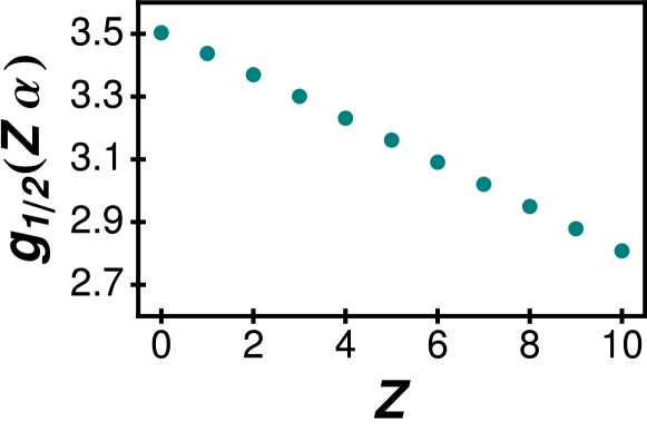
Figure 1: (Color online) We show the higher-order remainder function $g_{1/2}(Z\alpha)$ as a function of $Z$. Numerical values for $g_{1/2}(Z\alpha)$ are given in Table VII. The point at $Z=0$ is given by the coefficient $a_{20}(2P_{1/2})$.

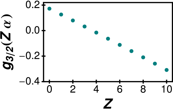
Figure 2: (Color online) Same as Fig. 1, but for the $2P_{3/2}$ state. The higher-order remainder function $g_{3/2}(Z\alpha)$ is plotted as a function of $Z$, with numerical values for $g_{3/2}(Z\alpha)$ given in Table VII. The point at $Z=0$ is $\lim_{Z\alpha\to 0}g_{3/2}(Z\alpha)=a_{20}(2P_{3/2})$.

VIII Final Results

Summarizing our calculations, we conclude that the QED correction to the HFS of $P$ states can be cast into the form

$$\Delta E_{nP_{j}}=E_{F}(nP_{j})\,\delta\xi_{e}(j)$$ (74)

$$=E_{F}(nP_{j})\frac{\alpha}{\pi}\left[a_{00}+(Z\alpha)^{2}\,\left(a_{21}\,\ln[(Z\alpha)^{-2}]+a_{20}\right)\right],$$

which is valid up to order $\alpha(Z\alpha)^{2}E_{F}$. According to Eq. (V), the results for the leading coefficients are

$$a_{00}(nP_{1/2})=\frac{1}{4}\,,\qquad a_{00}(nP_{3/2})=-\frac{1}{8}\,.$$ (75)

The logarithmic part of the correction, as given by Eq. (33), is

$$a_{21}(nP_{1/2})=-2\frac{n^{2}-1}{n^{2}}\,,\qquad a_{21}(nP_{3/2})=0\,.$$ (76)

In particular, there are no squared logarithmic terms. As follows from Eqs. (V), (61), (VI), and (73), the total nonlogarithmic contribution $a_{20}$ is the sum of a self-energy (SE) and a vacuum-polarization (VP) correction,

$$a_{20}=a^{\rm SE}_{20}+a^{\rm VP}_{20}\,.$$ (77a)

The results read

$$a^{\rm SE}_{20}(nP_{1/2})= \ \frac{19}{144}+\frac{7}{8\,n}+\frac{5}{16n^{2}}+2\frac{n^{2}-1}{n^{2}}\ln 2$$

$$\ +\beta(nP_{1/2})\,,$$ (77b)

$$a^{\rm VP}_{20}(nP_{1/2})= \ \frac{2}{5}\,\frac{n^{2}-1}{n^{2}}\,,$$ (77c)

$$a^{\rm SE}_{20}(nP_{3/2})= \ \frac{109}{2880}-\frac{11}{32\,n}+\frac{1}{30n^{2}}+\beta(nP_{3/2})\,,$$ (77d)

$$a^{\rm VP}_{20}(nP_{3/2})= \ 0\,.$$ (77e)

Using the results for the $\beta$ terms in Eqs. (69) and (71), we obtain, in particular,

$$a^{\rm SE}_{20}(2P_{1/2})= \;3.50343\,,$$ (78a)

$$a^{\rm SE}_{20}(2P_{3/2})= \;0.17198\,.$$ (78b)

These results can be compared to numerical data at low $Z$ presented in Ref. YeJe2009 .

Indeed, for low-$Z$ one-electron ions, a nonperturbative (in $Z\alpha$) calculation of the self-energy correction to the hyperfine splitting has recently been carried out YeJe2009 . The numerical values for the self-energy correction $\Delta E_{nP_{j}}$ to the hfs find a natural representation as

$$\Delta E_{nP_{j}}=E_{F}(nP_{j})$$

$$\times\frac{\alpha}{\pi}\left[a_{00}+(Z\alpha)^{2}\,\left(a_{21}\,\ln[(Z\alpha)^{-2}]+g_{j}(Z\alpha)\right)\right],$$

where $g_{j}(Z\alpha)$ is a remainder function which approaches the $a_{20}$ coefficient for $Z\alpha\to 0$,

$$\lim_{Z\alpha\to 0}g_{j}(Z\alpha)=a_{20}(nP_{j})\,.$$ (79)

Numerical values for the remainder functions $g_{j}(Z\alpha)$ are given in Table VII. In Figs. 1 and 2, we plot the higher-order remainder against the nuclear charge number $Z$. The numerical data are consistent with the next higher-order term in the expansion of $\Delta E_{nP_{j}}$ being a correction of order $\alpha(Z\alpha)^{3}$ (no logarithm).

IX Conclusions

The hyperfine structure of $P$ states is an interesting physical problem. In accurate measurements of the classical ($2P_{j}$–$2S$) Lamb shift in atomic hydrogen, both the hyperfine effects of $P$ as well as of $S$ states have to be carefully accounted for before a meaningful comparison of theory and experiment can be made. In alkali-metal atoms, the hyperfine structure of $P$ states is also of great experimental interest GeDeTa2003 ; WaEtAl2003 ; DaNa2006 .

In the present investigation, we analyze QED corrections to the hyperfine splitting of $nP_{1/2}$ and $nP_{3/2}$ states in hydrogenlike systems, up to order $\alpha(Z\alpha)^{2}E_{F}$, where $E_{F}$ is the Fermi splitting. Our calculation relies on the separation of the electronic from the nuclear degrees of freedom as described in Sec. II, effectively reducing the problem to an electronic self-energy type calculation. The identification of the nonrelativistic degrees of freedom relevant to our investigation is accomplished by the Foldy–Wouthuysen transformation as described in Sec. III. A nuclear-spin dependent correction to the electronic transition current is identified [see Eq. (22)]. We show (see Sec. IV) that squared logarithmic corrections of relative order $\alpha(Z\alpha)^{2}\ln^{2}[(Z\alpha)^{-2}]E_{F}$ are completely absent for $P$ states, whereas for $P_{3/2}$, even the single logarithmic term of relative order $\alpha(Z\alpha)^{2}\ln[(Z\alpha)^{-2}]E_{F}$ vanishes. This finding is interesting in view of different conjectures described in the literature SaCh2006 .

In order to address the nonlogarithmic correction of relative order $\alpha(Z\alpha)^{2}E_{F}$, we split the calculation into a high- and a low-energy part and match them via an intermediate overlapping parameter $\epsilon$ that separates the scales of high-energy and low-energy photons (see Secs. V and VI). This parameter is noncovariant but turns out to lead to a concise formulation of a problem which is otherwise rather involved. The high-energy part is treated in Sec. V and is seen to lead to form-factor type corrections. For the low-energy part treated in Sec. VI, the correction to the electron’s transition current induced by the hyperfine interaction is crucial. This correction can be obtained via a Foldy–Wouthuysen transformation (Sec. III). The discussion of vacuum-polarization corrections (see Sec. VII) and a brief summary of the results obtained (Sec. VIII) conclude our investigation.

We reemphasize once more that the logarithmic $a_{21}$ coefficient vanishes for $P_{3/2}$ states [see Eq. (34)], and the $a^{\rm SE}_{20}$ self-energy coefficient [see Eq. (78b)] also is numerically small for $2P_{3/2}$. These two observations account for the numerically small results obtained in the all-order calculation YeJe2009 for the self-energy corrections to the HFS of this state. Indeed, the QED self-energy corrections to the hyperfine splitting of $2P_{3/2}$ states are surprisingly small at low $Z$. This behaviour is naturally attributed to the less singular behaviour of the $P_{3/2}$ states at the origin in comparison to that of the $P_{1/2}$ states.

Acknowledgments

U.D.J. has been supported by the National Science Foundation (Grant PHY–8555454) as well as by a Precision Measurement Grant from the National Institute of Standards and Technology. V.A.Y. was supported by DFG (grant No. 436 RUS 113/853/0-1) and acknowledges support from RFBR (grant No. 06-02-04007) and the foundation “Dynasty.”

References

- (1) P. J. Mohr, G. Plunien, and G. Soff, Phys. Rep. 293, 227 (1998).
- (2) P. J. Mohr, Ann. Phys. (N.Y.) 88, 26 (1974).
- (3) P. J. Mohr, Ann. Phys. (N.Y.) 88, 52 (1974).
- (4) A. Gumberidze, T. Stöhlker, D. Banás, K. Beckert, P. Beller, H. F. Beyer, F. Bosch, S. Hagmann, C. Kozhuharov, D. Liesen, F. Nolden, X. Ma, P. H. Mokler, M. Steck, D. Sierpowski, and S. Tashenov, Phys. Rev. Lett. 94, 223001 (2005).
- (5) U. Jentschura and K. Pachucki, Phys. Rev. A 54, 1853 (1996).
- (6) K. Pachucki, Ann. Phys. (N.Y.) 226, 1 (1993).
- (7) L. L. Foldy and S. A. Wouthuysen, Phys. Rev. 78, 29 (1950).
- (8) G. W. Erickson and D. R. Yennie, Ann. Phys. (N.Y.) 35, 271, 447 (1965).
- (9) K. Pachucki, A. Czarnecki, U. D. Jentschura, and V. A. Yerokhin, Phys. Rev. A 72, 022108 (2005).
- (10) U. D. Jentschura and K. Pachucki, J. Phys. A 35, 1927 (2002).
- (11) U. D. Jentschura, P. J. Mohr, and G. Soff, Phys. Rev. Lett. 82, 53 (1999).
- (12) M. Niering, R. Holzwarth, J. Reichert, P. Pokasov, Th. Udem, M. Weitz, T. W. Hänsch, P. Lemonde, G. Santarelli, M. Abgrall, P. Laurent, C. Salomon, and A. Clairon, Phys. Rev. Lett. 84, 5496 (2000).
- (13) M. Fischer, N. Kolachevsky, M. Zimmermann, R. Holzwarth, Th. Udem, T. W. Hänsch, M. Abgrall, J. Grünert, I. Maksimovic, S. Bize, H. Marion, F. Pereira Dos Santos, P. Lemonde, G. Santarelli, P. Laurent, A. Clairon, C. Salomon, M. Haas, U. D. Jentschura, and C. H. Keitel, Phys. Rev. Lett. 92, 230802 (2004).
- (14) U. D. Jentschura, P. J. Mohr, and G. Soff, Phys. Rev. A 63, 042512 (2001).
- (15) V. A. Yerokhin, P. Indelicato, and V. M. Shabaev, Phys. Rev. A 69, 052503 (2004).
- (16) S. A. Blundell, K. T. Cheng, and J. Sapirstein, Phys. Rev. Lett. 78, 4914 (1997).
- (17) P. Sunnergren, H. Persson, S. Salomonson, S. M. Schneider, I. Lindgren, and G. Soff, Phys. Rev. A 58, 1055 (1998).
- (18) V. A. Yerokhin and V. M. Shabaev, Phys. Rev. A 64, 012506 (2001).
- (19) K. Pachucki, Phys. Rev. A 54, 1994 (1996).
- (20) M. Nio and T. Kinoshita, Phys. Rev. D 55, 7267 (1997).
- (21) J. Sapirstein and K. T. Cheng, Phys. Rev. A 74, 042513 (2006).
- (22) J. Sapirstein and K. T. Cheng, Phys. Rev. A 78, 022515 (2008).
- (23) V. A. Yerokhin and U. D. Jentschura, Self-energy correction to the hyperfine splitting and the electron factor in hydrogen-like ions, Phys. Rev. A, submitted.
- (24) S. J. Brodsky and R. G. Parsons, Phys. Rev. 176, 423 (1968).
- (25) U. D. Jentschura and V. A. Yerokhin, Phys. Rev. A 73, 062503 (2006).
- (26) K. Pachucki, Phys. Rev. A 53, 2092 (1996).
- (27) D. Zwanziger, Phys. Rev. 121, 1128 (1961).
- (28) K. Pachucki, Phys. Rev. A 71, 012503 (2005).
- (29) J. D. Bjorken and S. D. Drell, Relativistische Quantenmechanik (Bibliographisches Institut, Mannheim, Wien, Zürich, 1966).
- (30) U. D. Jentschura, Master Thesis: The Lamb Shift in Hydrogenlike Systems, [in German: Theorie der Lamb–Verschiebung in wasserstoffartigen Systemen], (University of Munich, 1996, unpublished (see e-print hep-ph/0305065)).
- (31) C. Itzykson and J. B. Zuber, Quantum Field Theory (McGraw-Hill, New York, 1980).
- (32) V. M. Shabaev, J. Phys. B 24, 4479 (1991).
- (33) V. M. Shabaev, in Precision Physics of Simple Atomic Systems – Lecture Notes in Physics Vol. 627, edited by S. G. Karshenboim and V. B. Smirnov (Springer, Berlin, 2003), pp. 97–113.
- (34) V. Gerginov, A. Derevianko, and C. E. Tanner, Phys. Rev. Lett. 91, 072501 (2003).
- (35) J. Walls, R. Ashby, J. J. Clarke, B. Lu, and W. A. van Wijngaarden, Eur. Phys. J. D 22, 159 (2003).
- (36) D. Das and V. Natarajan, J. Phys. B 39, 2013 (2006).