On the basic computational structure of gene regulatory networks

Abstract

Gene regulatory networks constitute the first layer of the cellular computation for cell adaptation and surveillance. In these webs, a set of causal relations is built up from thousands of interactions between transcription factors and their target genes. The large size of these webs and their entangled nature make difficult to achieve a global view of their internal organisation. Here, this problem has been addressed through a comparative study for Escherichia coli, Bacillus subtilis and Saccharomyces cerevisiae gene regulatory networks. We extract the minimal core of causal relations, uncovering the hierarchical and modular organisation from a novel dynamical/causal perspective. Our results reveal a marked top-down hierarchy containing several small dynamical modules for E. coli and B. subtilis. Conversely, the yeast network displays a single but large dynamical module in the middle of a bow-tie structure. We found that these dynamical modules capture the relevant wiring among both common and organism-specific biological functions such as transcription initiation, metabolic control, signal transduction, response to stress, sporulation and cell cycle. Functional and topological results suggest that two fundamentally different forms of logic organisation may have evolved in bacteria and yeast.

I Introduction

The pattern of regulatory interactions linking transcription factors (TFs) to their target genes constitutes the first level of a multilayered network of gene regulation; the so called gene transcriptional regulatory networks (GRN) (Babu et al., 2004). Some of these patterns have been recovered from genome-wide approaches, particularly well established for Escherichia coli (Thieffry et al., 1998; Dobrin et al., 2004; Shen-Orr et al., 2002) and Bacillus Subtilis (Harwood and Moszer, 2002; Sellerio et al., 2009) as well as the unicellular eukaryote Saccharomyces cerevisiae (Lee et al., 2002; Balaji et al., 2006a). In such a picture, both hierarchical (Cosentino-Lagomarsino et al., 2007; Yu and Gerstein, 2006; Salgado et al., 2001) and modular (Resendis-Antonio et al., 2005; Wolf and Arkin, 2003; Balaji et al., 2006a; Freyre-González et al., 2008) components have been repeatedly highlighted, although no general agreement exists on what scale of analysis more accurately captures global complexity (Bornholdt, 2005).

The conceptualisation of cellular interaction maps within the framework of graph theory (Albert, 2005; Zhu et al., 2007; Babu et al., 2004) has provided powerful insights on their hierarchical (Clauset et al., 2008; Trusina et al., 2004; Vázquez et al., 2002; Sales-Pardo et al., 2007), modular organisation (Ravasz et al., 2002; Rodríguez-Caso et al., 2005; Palla et al., 2005; Newman, 2004) as well as it sheds light on the topological constraints imposed in its dynamical behaviour (Kauffman et al., 2003; Lee et al., 2002). However, their quantification, even their identification has led to a nonuniform concept of module under functional, topological, evolutionary and developmental criteria (Wagner et al., 2007; Hartwell et al., 1999). Similarly, the observed hierarchy seldom matches an ideal feed-forward relation between components (Whyte et al., 1969).

An alternative approach considers looking at GRNs in a more fundamental way, namely as sets of causal relations, featured by the directed nature of the link between a transcription factor with its target genes (Cosentino-Lagomarsino et al., 2005; Babu et al., 2004). Causal links, namely who acts on whom, allows to actually define the skeleton underlying dynamics by attending to the cyclic and linear nature of the genetic circuits.

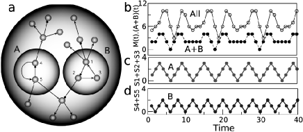
Figure 1: A small toy model (a) and its dynamic behaviour. The observed pattern is generated by the activity of two basic feedback loops, indicated as $A$ and $B$ in (a). These subsets are responsible for the qualitative dynamics exhibited by the net, as shown in (b) with filled circles. Moreover, this attractor results from the combination of the two different periodic orbits displayed by the two basic modules, whose time series are shown in (c-d). For a mathematical treatment of this specific example see appendix.

Figure 1 illustrates the resulting dynamics of a toy model (see mathematical appendix for formal details). In this model we observe that the complex, periodic behaviour may arise solely due to the dynamics of the two subgraphs (A and B in figure 1a) exhibiting feedback loops. The remaining system simply reacts to the dynamical inputs generated from these modules. Interestingly, these mentioned topological traits defines the dynamical behaviour no mattering what kind of dynamical rules are used to causally relate our elements. Some elements will play the leading role, determining the qualitative type of dynamics, whereas others will just amplify or reduce the core signals. This view of interactions is at the core of a relational picture of a biological computation (Rosen, 1991). This is a computational perspective and, not surprisingly, GRNs have been compared to computers (Hogeweg, 2002; Istrail et al., 2007; Bray, 1995; Rosen, 1991; Macía and Solé, 2009). Cellular computations pervade both the diverse responses to external stimuli (Luscombe et al., 2004; Balázsi et al., 2005) as well as cell robustness and plasticity (Aldana et al., 2007; Lee and Rieger, 2007; Shmulevich et al., 2005). A number of dynamical approximations suggest a link between network organization and its dynamical behaviour. However, due to the large size of these systems, only a few small ones (Li et al., 2004; Espinosa-Soto et al., 2004) have been fully analysed.

Ideally, it would be desirable to have a method to construct a graph capturing all non-trivial causal relations and thus all potentially important computational links. In this paper we show that such organisation of GRNs is captured by the principle of causality depicted by the directed nature of gene-gene relations. This can uncovered by exploiting the properties of directed graphs, in particular, by the use of leaf removal algorithms (LRAs) (Sellerio et al., 2009; Cosentino-Lagomarsino et al., 2005) and the identification of the so-called strongly connected components (SCCs) (Gross and Yellen, 1998). As we will see, LRAs recover the network fraction responsible for potentially non trivial computations. Furthermore, the internal organisation of this especial subgraph can be topologically dissected by SCC identification.

A SCC is defined for a set of vertices if there is a walk -attending to the directedness of edges- from each vertex to every other vertex of this set (see figure 2). The identification of SCC has been applied to a diverse number of systems from the Internet (Broder et al., 2000) to metabolism and neural wiring network (Serrano and De Los Rios, 2008). Recently, it has been described that yeast GRN presents a giant SCC (Jeong and Berman, 2008), contrasting with an acyclic and feed-forward organisation of E. coli (Ma et al., 2004).

In this work, we explore the topological constraints derived from wiring patterns of causal dependencies in a comparative analysis of yeast, E. coli and B. subtilis by defining their qualitatively relevant causal cores. We explore their internal organisation in terms of irreducible computational entities at the level of gene regulatory systems. As will be shown below, our analysis (using a more updated version of E. coli GRN) revealed relevant differences in relation to previous results published in the literature.

II Results

II.1 Causality, dynamics and topology

Causal relations in GRNs can be described in terms of directed graphs (in short digraphs) (Babu et al., 2004; Albert, 2005). A graph is constituted by a set of vertices or nodes (here the genes) and the set of edges linking them (the relations among genes). The regulatory effect of a TF gene $v_{i}$ on a specific target gene $v_{j}$ is depicted by an arrow ($v_{i}\rightarrow v_{j}$) in the graph plot.

If the vertices are genes, a chain of connections of different TFs corresponds in graph theory with a directed walk and it can be interpreted as a causal chain. Interestingly, all TFs exhibit outgoing links, whereas non-TF genes (the target ones) only receive arrows from the TF set. The number of outgoing links of a vertex is known as out-degree (denoted by $k_{out}$) whereas the number of incoming edges is the in-degree ($k_{in}$). Since a TF can be a regulatory target of other TFs, they can exhibit both incoming and outgoing links, allowing feed-backs to occur.

A specially important information about the organization of directed graphs is provided by the analysis of its connected components, i.e. the graph in which every pair of distinct vertices has a walk -see appendix. In digraphs, directed walks are non trivially organised. The Internet is a very illustrative example of that (Broder et al., 2000) exhibiting a bow-tie structure with three different connected components: 1) a central strongly connected component (SCC), namely a subgraph for which every two vertices are mutually reachable (Gross and Yellen, 1998; Dorogovtsev and Mendes, 2003), 2) a set of incoming components ($IC$) composed by the set of feed-forward pathways starting from vertices without in-degree and ending in SCC and 3) a set of outgoing components ($OC$) where pathways starting from SCC end in vertices without out-degree (see figure 2).

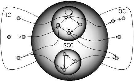
Figure 2: Bow-tie structure depicting an incoming component ($IC$), two strongly connected components (SCCs) and the outgoing component ($OC$).

Typically, the pattern of activation of a given gene has a time-dependent causal relation with the state of the set of genes affecting it, and every vertex $v_{i}$ can acquire a given state from a number of possible states. Specifically, the state of $v_{i}$ at time $(t+1)$ is influenced by the state of the vertices affecting it at time $t$ -see appendix. The equations describing the dynamical behaviour of a given vertex $v_{i}$ at time $t+1$ can be formulated in different ways, including Boolean dynamics (Thomas, 1973; Kauffman, 1993), threshold nets (Li et al., 2004) as figure 1 illustrates or coupled differential equations (de la Fuente and Mendes, 2002). These models are different but all show a common principle of causality: the state of a given vertex $v_{i}$ at time $t+1$ is exclusively defined by the vertices affecting it at time $t$. No matter our choice of the dynamical equations, the patterning of links must strongly influence system’s behaviour.

The presence of a cyclic walk -a directed walk where the first and the ending vertices are the same- is a necessary (but not sufficient) requisite for a periodic solution. This is due to the fact that, in interpreting directed edges as causal relations, a cyclic graph implies that every vertex is indirectly affected by itself. When we consider the whole graph, an overlapping of cycles originates the SCC set that can be governed by the $IC$ set. As we shall show below, these two structures represent the core of the graph that qualitatively constrains its dynamical complexity. By contrast, in linear directed walks, the upstreamest element fully determines the final state of the elements belonging to this walk.

A set able to properly capture the relevant components qualitatively affecting global behaviour should remove linear paths from the graph. Under this view, we can identify this set by means of a straightforward iterative algorithm. Given the underlying influence of causal relations on system’s dynamics, we will use the label dynamic for most of our definitions.

II.2 Dynamical backbone

We compute the dynamical backbone ($DB$) of a given directed graph ${\cal G}$ (to be noted $DB({\cal G})$) by the iterative pruning of vertices with $k_{out}=0$ from the initial graph, but maintaining those vertices whose $k_{in}=0$ (figure 3). This algorithm belongs to the family the so-called leaf removal algorithms (Bauer and Golinelli, 2001; Correale et al., 2006; Cosentino-Lagomarsino et al., 2007) that have been previously used for the analysis of GRNs (Kauffman et al., 2003; Cosentino-Lagomarsino et al., 2007; Sellerio et al., 2009).

Figure 3a illustrates the mechanism of pruning. Notice that, in contrast with previous proposals of leaf-removal algorithms, the $DB({\cal G})$ also keeps the single root vertices i.e. those such that $k_{in}=0$ which appear isolated. Single root vertices are special because their state is only externally changed and are not influenced by other genes. We observe that, in general the $DB({\cal G})$ displays more than a single connected component (see figure (3)). Interestingly, this dynamically relevant subgraph coincides with the union of the previously described $IC$ and SCC sets of a directed graph. By contrast, $OC$ is associated with another interesting subgraph, to be indicated as $DB^{\prime}({\cal G})$ formed by the fraction of the net that exclusively displays feed-forward structures. See appendix for its formal construction.

The application of the above defined algorithm leads to a drastic reduction of network complexity, preserving the computational structures responsible of the qualitative behaviour of the net.

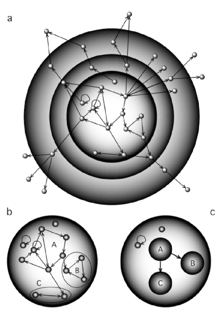
Figure 3: Dynamical Backbone definition. (a) an example of the iterative elimination of vertices without out-degree ($k_{out}=0$). Different layers indicate the successive iterations of the algorithm. In (b) we indicate the dynamical modules of the $DB({\cal G})$. Maximal cycles larger than one vertex are labelled by capital letters. Figure (c) shows the hierarchical organization of the collapsed dynamical modules, i.e., the feed-forward organization obtained after the condensation of the graph $DB({\cal G})$ -see text. Notice that the $DB({\cal G})$ exhibits isolated self-interacting vertices that, by definition, are dynamical modules but auto-loops are maintained in order to provide a more informative picture.

II.3 Dynamical Modules and Hierarchy

As we argued above, the core of causal relations of a GRN is captured by its $DB$. Furthermore, the causal relations inside this $DB$ can display some kind of hierarchy. As we shall see $DB$ organisation can be studied by SCC detention and the so-called graph condensation process. Mathematical appendix formally details the treatment of GRNs that uncovers the order relation (i.e. the hierarchical order) among the elements of the net.

Figure 3b illustrates the process for module identification by SCC detection. Interestingly, the nodes belonging to a SCC are mutually affected and therefore, they all contribute to the state definition of all the set (see A and B regions of the toy model described in figure 1a). The complexity of these topological entities cannot be reduced and thus, SCC concept defines an irreducible unit of causal relations (see mathematical appendix for formal definition). In this sense, the SCC can be identified with the module concept, since it constitutes an identifiable semiautonomous part of the system (Wagner et al., 2007), capturing a part of the dynamical complexity of the system. Therefore, we say that, within the context of GRNs, SCCs represent a sort of dynamical modules. We finally note that, consistently with definition, a single vertex belonging to the $DB$ but not participating in any cycle is itself a dynamical module.

Interestingly, when the SCC is represented by a single vertex, the resulting graph is a directed acyclic graph (see figure 3c). Such an operation is commonly referred in the literature as the condensation of a graph (Gross and Yellen, 1998).

The result after the condensation process is precisely the feed-forward organisation what enables us to define an order relation among the elements of the $DB$. It is worth stressing that an order relation cannot be established in cyclic wiring. Condensation process allows us to identify such cycles into SCCs representing dynamical modules. In this way, the internal organisation in a hierarchy of causal relations is revelaled for the $DB$.

II.4 E. coli dynamical backbone

Table 1: A selection of statistically over-represented biological functions terms from gene ontology annotation (GOA) is shown for $DB$, the root node set and dynamical modules (A to E), accordingly functional analysis for E. coli. Notice that three genes of the $DB$ were not found in GOA annotation (see SI2 for a detailed analysis). The number of genes belonging to a specific GOA term is depicted in the first column. The fraction of genes associated to specific GOA respecting to the total number of genes for each particular set are shown for $P>0.05$ ($P$ is the level of significance). Highly significant results ($P<10E-5$) are indicated with (**). Values within the interval of $10E-5>P>10E-3$ are marked by (*).

Biological Function	$\#$ genes in GO	Fraction of the GO term in the analysed set
		E. coli DB	Root nodes	DM A	DM B	DM C	DM D	DM E
Regulation of
transcription,	354	135/136*	37/37*	10/11*	4/4**	3/3	2/2	2/2
DNA-dependent
Regulation of metabolism	399	136/136	37/37**	11/11*	4/4**	3/3	2/2	2/2
Two-component signal
transduction system	91	26/136*	6/37**	–	–	–	–	–
(phosphorelay)
Transcription initiation	7	7/136*	–	4/11*	1/4	–	–	–
Negative regulation of
cellular process	36	10/136*	4/37**	2/11	–	–	–	–
DNA replication	62	–	–	3/11**	–	–	–	–
Response to heat	4	–	–	1/11	–	–	–	–
Response to antibiotic	60	–	–	–	–	2/3	–	–
Carbohydrate transport	112	–	–	–	–	–	2/2	–

We extracted the GRN for E. coli K-12 prokaryote from the available information in RegulonDB 6.0 database (Gama-Castro et al., 2008). The resulting network was a directed graph with 1607 vertices ($43$ of them with $k_{in}=0$) and 4141 links with a giant component of 1589 vertices and average degree $\langle k\rangle=5.1$ [See Methods for network construction]. The network included a total of 156 vertices with $k_{out}>0$, corresponding with transcription and $\sigma$ trans-acting factors, and 1451 vertices with $k_{out}=0$, i.e, the target genes.

From the E. coli GRN, the $DB$ subgraph was obtained after the second iteration of the algorithm. The $DB$ subgraph consists of $142$ vertices ($8.9\%$ of the GRN) distributed as follows: $33$ single root vertices and a set of subgraphs with $109$ vertices ($10$ of them with $k_{in}=0$) and $279$ edges. This set is organised in $9$ graphs: a giant component of $100$ vertices ($\langle k\rangle=3.7$), another component displaying two elements and $7$ isolated self-interacting vertices. We found that the size of the studied $DB$ is markedly smaller than the expected in a null model obtained by randomisation process. In this methodology, node degree is conserved but correlations among nodes are destroyed (see methods section). Differences in the $DB$ size between E. coli and randomised counterpart feature the biological fact of that only a small fraction of genes in the genome operates over a majority of genes without a direct role in the regulation of transcription. As expected and in agreement with the direct observation of RegulonDB, the genes belonging to $DB$ are described as either transcription or $\sigma$ factors. Only two exceptions were found: the transcription anti-terminator cspE and trmA, a tRNA metyltransferase (according to RegulonDB 6.0 [see SI for a biological function of $DB$ genes]). Functional analysis based on gene ontology annotation confirmed the significant ($P<10E-5$) overabundance of general functions related to regulation of transcription, signal transduction and transcription initiation (see table LABEL:Ecoli_table and SI2 for a detailed statistical analysis).

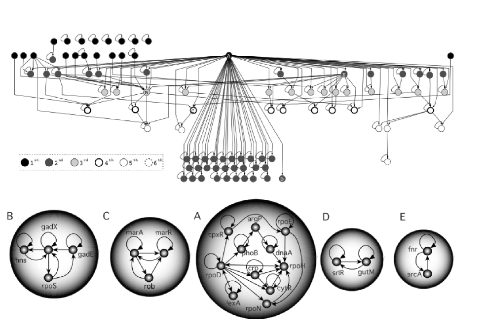
Figure 4: Dynamical hierarchy and modularity of E. coli GRN. Dynamical Backbone of E. coli after collapsing dynamical modules revealing a causal hierarchy (above). Different levels of downstream information processing are indicated by means of different vertex labelling. Dynamical modules larger than one vertex are represented by an individual node labelled by capital letters. Auto-links in single-node module are preserved in the graph for a more informative picture. Below E. coli $DB$, the five (A to E) dynamical modules larger than one node are shown.

Figure 5: Randomisation for E. coli GRN and its respective TF-TF subgraph (figure insets). Normalised counts represent the number of times that a value of the measured estimator ($DB$ size, number of root nodes and SCC size) appears, normalised by the number of repetitions (1000 randomised networks)

Concerning the previous observations, we obtained a graph resulting from the interactions among TFs (topologically, the nodes with out-degree) in GRN. According its definition, $DB$ is also a subset of TF subnet. Figure 5a inset shows that $DB$ size for randomised TF-TF subgraph is fairly smaller than the E. coli $DB$. We also found that the number of root nodes expected by chance in both GRN and TF subgraph follow a similar behaviour than the observed for $DB$ size. These results show that $DB$ structure for $E.coli$ exhibits a markedly different organisation than the expected in a null model (see figure 5b).

Figure 4a shows the $DB$ organisation after the condensation process. The analysis of the condensed $DB$ revealed five dynamical modules larger than one vertex (figure 4b). Interestingly, the size of SCCs are markedly smaller in both GRN and TF randomised sets. Notice that figure 5 depicts large values for SCC sizes equal to one in randomised networks, however, they correspond with the fraction of the non condensed network. Typically, randomised networks exhibited a single large SCC component (within the range of 800-900 nodes), occasionally together with a very small SCC, rarely larger than three nodes (data from SCC distributions within networks are not shown). It is worth to note that no randomised web, neither for GRN nor TF-TF subgraph sets produced exclusively small SCCs as observed in real data. This indicates that GRN is not devoid of cycles but they are distributed along the $DB$ and confined in dynamical modules of small size.

We found that the condensed $DB$ captures the hierarchical behaviour of the largest graph component evidenced by a feed-forward order relation with six layers of downstream dependencies (see figure 4). By definition, the first layer contains all the vertices with $k_{in}=0$ but we can see that it also includes the largest dynamical module.

The largest module (A in figure 4) contains four of the seven $\sigma$ factors described for E. coli (see table LABEL:Ecoli_table and SI2 for statistical details). These elements are responsible for transcription initiation. Together with the primary initiator factor rpoD ($\sigma^{70}$), we found the alternative ones operating under heat shock stress (rpoH and rpoE, corresponding with $\sigma^{32}$ and $\sigma^{24}$, respectively). In addition, rpoN ($\sigma^{54}$, initiator of nitrogen metabolism genes) is also part of the module. The second largest hub (a highly connected vertex) in the $DB$ is the crp gene, also known as CAP (catabolite activator protein). CAP is a general regulator that exerts a positive control of many of the catabolite sensitive operons as a sensor of glucose starvation. Interestingly, the members of module A participates in the $44\%$ of the total number of links of the GRN, indicating the relevance of this module in defining the state of the whole network.

Other relevant factors are co-localised in this dynamical module such as those TFs related to nutrient sensor and assimilation (phosphate sensor system, phoB, as well as nucleoside (cytR) and arginine (argP) transport control. Notice that the initiator factor of DNA replication initiator (dnaA) is associated with this group, and we also found two specific TF expressed under stress conditions (lexA and cpxR). Similarly, the other four modules include key genes associated to adaptive responses to changing environmental clues. These include homeostasis in acid environment (stress responses to high osmolarity, module B), antibiotic resistance (lead by marA and marR, module C), glucitol use (module D) or responses to oxygen changes (module E).

In summary, the E. coli $DB$ describes a hierarchical feed-forward network with a strong fan-like pattern dominated by a single irreducible subset of TFs. This pattern reveals, in terms of a computational design, a strongly centralised organisation, with a well defined node affecting multiple layers of activity. The largest hub has no input from other members of the $DB$ and thus only affect to other’s behaviour. Within the $DB$, we identify the dynamical modules responsible for the control of transcriptional replication under both normal and stress conditions, control of metabolism, DNA replication as well as assimilation of essential sources of nitrogen and phosphorous.

II.5 B. subtilis dynamical backbone

Table 2: A selection of statistically over-represented biological functions terms from gene ontology annotation (GOA) is shown for $DB$, the root node set and dynamical modules (A to E), accordingly functional analysis for B. subtilis. The number of genes belonging to a specific GOA term is depicted in the first column. Notice that 8 genes of 144 belonging to $DB$ were not found in GOA and therefore not considered in this analysis. The fraction of genes associated to specific GOA respecting to the total number of genes for each particular set are shown for $P>0.05$ ($P$ is the level of significance). Highly significant results ($P<10E-5$) are indicated with (**). Values within the interval of $10E-5>P>10E-3$ are marked by (*).

Biological Function	$\#$ genes in GO	Fraction of the GO term in the analysed set
		B. subtilis DB	Root nodes	DM A	DM B	DM C	DM D	DM E
Regulation of
transcription,	357	113/121*	58/62*	2/2	2/2	2/2	2/2	3/3
DNA-dependent
Regulation of metabolism	368	114/121*	58/62*	2/2	2/2	2/2	2/2	3/3
Two-component signal
transduction system	99	8/121*	12/62*	–	–	2/2	–	–
(phosphorelay)
Transcription initiation	26	14*	5/62**	2/2	2/2	–	–	1/3
Negative regulation of
cellular process	15	8/121*	3/62	–	–	–	–	–
Positive regulation of
cellular process	8	6/121*	6/62*	–	–	–	–	–
Transcription termination	6	3/121	2/62**	–	–	–	–	–
Sporulation	258	–	–	–	2/2	–	–	3/3
Phosphate transport	10	–	–	–	–	1/2	–	–

B. subtilis GNR was obtained from DBTBS (Sierro et al., 2008) [see Methods for network construction]. The resultant network consists of 922 nodes (159 with $k_{out}>0$, 83 of them with $k_{in}=0$ and 763 with $k_{out}=0$) and 1366 directed links ($\langle k\rangle=2.96$). A component of 892 nodes was predominant and the remaining nodes made part of very little isolated subgraphs (one of five nodes, one of three, 10 of two nodes and two isolated self-interacting nodes).

The computation of $DB$ required four iterations before the acquisition of the stable graph. The process removed 778 nodes, resulting a $DB$ of 144 genes (10.5 % of the GRN) . In this set, 73 were isolated root nodes and 71 nodes were distributed in 8 connected components (a big one of 59 nodes, one of five, one of two and 5 self-interacting isolated nodes) with 108 links. Analogously to the observed for E. coli, statistical analysis of GOA terms showed and over-abundance of regulation of transcription metabolism and cell signalling (see table LABEL:Bsubtilis_table and SI2 for statistical details) in both $DB$ and root nodes set (see table LABEL:Bsubtilis_table and SI2 for statistical details). Other functions relating to transcription termination and positive regulation process appear in B. subtilis $DB$.

We note that comparison of functional analysis among species must be taken with caution due to the different coverage of genes in GOA terms that may produce a bias in the interpretation of results. In order to provide a more complete picture, we consider functional information annotated in DBTBS. However, we cannot exclude some discrepancies derived from the use of different sources. Similarly to E. coli, statistical functional analysis is complemented by a direct function examination of the genes belonging to $DB$ in DBTBS (see SI for functional information).

Concerning to null model comparison, figures 7a and b suggest a similar behaviour for $DB$ and the set of root nodes in randomised networks than the observed for E. coli.

SCC calculation revealed five dynamical modules as illustrated in figure 6. Four of them in the same 54-connected component and the other one in the 5-component component. Similarly to E. coli, a single markedly large SCC is expected in randomised networks (see figure 7c). In the same way, the acyclic graph resulting by SCCs condensation revealed a strong hierarchical character, similar to its E. coli bacterial counterpart. In this case, module A consisted of a cross-regulation of sigA and sigD sigma factors. These two nodes participates in the $26\%$ of the total number of links of the GRN. This agrees with the essential role of these genes. SigA, also known as $\sigma^{43}$ or rpoD, is an essential gene, primary $\sigma$ factor of this bacterium. It is also worth nothing that the equivalent rpoD gene occupies a similar position on the top of the E. coli condensed $DB$ (module A in figure 4). The module partner of this gene in B. subtilis, sigD or $\sigma^{28}$, is a sigma factor required for flagellum and motility genes involved in chemotaxis process. This is different from E. coli, since its equivalent gene fliA (also $\sigma^{28}$) does not belongs to the E. coli module A but it has a direct downstream dependence of this module.

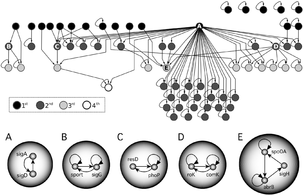
Figure 6: Dynamical hierarchy and modularity of B. subtilis GRN. Dynamical Backbone of B. subtilis after collapsing dynamical modules revealing a causal hierarchy (above). Different levels of downstream information processing are indicated by means of different vertex labelling. Dynamical modules larger than one vertex are represented by an individual vertex labelled by capital letters. Auto-links in single-node module are preserved in the graph for a more informative picture. Below B. subtilis $DB$, the five (A to E) dynamical modules larger than one node are shown.

As illustrated in figure 6, modules C and D receive a direct input from the master module A. They appear related to signal transduction systems (resD and comk in module C and D, respectively). Interestingly, a cross dependence between respiration and phosphate assimilation is captured in module C. It has been described that resD can also play a regulatory role in respiration whereas phoD makes part of a molecular system involved in the regulation of alkaline phosphatase and phosphodiesterase alkaline phosphate, two enzymes involved in the uptake of free phosphate groups from the environment. Moreover, a catabolite repression factor, ccpA, responsible for the repression of carbohydrate utilisation and the activation of excretion of excess carbon affects this module. This suggests a strong relation between phosphorous and carbon assimilation with respiratory regulation. In other hand, the rok-comk genetic circuit described in module E appears involved in the expression of the late competence genes.

In contrast to what occurs in E. coli, the most complex module is not at the top of the hierarchy. Module E is a three component gene (much smaller than for E. coli) closely related to sporulation process. It is noteworthy that this module receives inputs from the competence-related module E and another sporulation module (see table LABEL:Bsubtilis_table) is found in an independent component. This is the case of module B which does not belong to the same $DB$ connected component of the remaining modules. It contains a sporulation-specific $\sigma$ factor (sigG, together with spovT controlling factor). Interestingly, this module, significantly associated to sporulation function (see Table LABEL:Bsubtilis_table), is affected by another sporulating $\sigma$ factor (sigF). Another relevant trait is the link between sporulation and response to nutritional stress performed by spo0A and the catabolite repression role of abrB in module D.

From a topological point of view, the most obvious difference between E. coli and B. subtilis is the simpler composition of dynamical modules for bacillus. We must stress that the knowledge of these organisms -specially for B. subtilis, which is much less known that its E. coli counterpart- is in constant advance. Thus, a variation in the wiring of these modules cannot be neglected. However, differences in module conformation might also be due to the large phylogenetic distance among these bacteria, as well as the extremely different environments where they live. E. coli is a gram-negative enterobacteria unable to sporulate that lives in the intestine of warm animals, whereas B. subtilis is a free living gram-positive organism, usually found in soils and with the ability to sporulate. However, in spite of these differences, a very similar architecture with a strong hierarchical character of its $DB$ is shared. Once again, a single only-output hub is observed. As show below, this is markedly different from what is found in our eukaryotic example.

Figure 7: Randomisation for B. subtilis GRN and its respective TF-TF subgraph (figure insets). Normalised counts represent the number of times that a value of the measured estimator ($DB$ size, number of root nodes and SCC size) appears normalised by the number of repetition (1000 randomised networks)

II.6 Yeast dynamical backbone

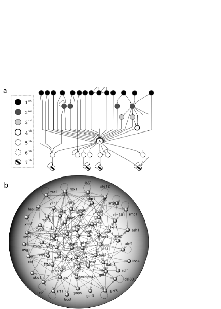
Figure 8: Dynamical hierarchy and modularity of Saccharomyces cerevisiae GRN. Dynamical Backbone of yeast after collapsing dynamical modules (above). One single dynamical module is represented by a vertex labelled by A letter. Below, the A dynamical module. As in the other diagrams, box legend shows the levels of computation.

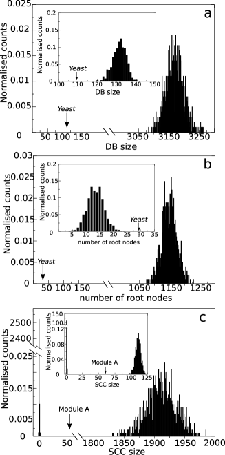
Figure 9: Randomisation for B. subtilis GRN and its respective TF-TF subgraph (figure insets). Normalised counts represent the number of times that a value of the measured estimator ($DB$ size, number of root nodes and SCC size) appears normalised by the number of repetition (1000 randomised networks)

GRN of Saccharomyces cerevisiae eukaryote was obtained from a compilation of different genome scale transcriptional analyses (Balaji et al., 2006a) [see Methods for network construction]. The resulting network was a directed graph consisting of a single connected component with 4441 vertices (29 of them with $k_{in}=0$) and 12900 links, leading to a $\langle k\rangle=5.8$. The network included a total of 157 vertices with $k_{out}>0$ and $4284$ vertices with $k_{out}=0$, corresponding with the transcription factors and targets genes analysed in the different datasets compiled in (Balaji et al., 2006a).

The yeast $DB$ subgraph was obtained after three iterations of $DB$ pruning. The $DB$ was formed by a set of $109$ vertices ($2.45\%$ of the GRN), being $17$ of them isolated single root vertices, and a single connected component displaying 92 vertices and 318 edges, leading to $\langle k\rangle=6.1$. Analogously to bacteria GRNs, randomisation process produced networks with much larger $DB$ with a smaller number of root nodes and a very large SCC compared to real yeast $GRN$ (see figure 9). However, a different behaviour was observed from yeast TF-TF subgraph producing a fairly bigger $DB$ after randomisation process. This suggests that although bacteria and yeast $DB$ exhibited a similar size, they would differ in their $DB$ organisation.

Functional analysis revealed that $DB$ consists of elements responsible for regulation of transcription and metabolism as observed in bacteria. In addition cell cycle related functions and response to chemical stimulus appeared significantly over-represented in $DB$, the root node set and SCC (see table LABEL:yeast_table and SI2 for detailed statistical analysis).

All the 109 genes of the $DB$ appear included in the list obtained from (Balaji et al., 2006a) defining the TF genes of the yeast GRN. In addition, we checked that all $DB$ elements, but five were clearly identified as TFs in the current version Saccharomyces genome database (Hong et al., 2008). However, they all were classified as regulators of gene expression [See SI for biological details of $DB$ genes].

The condensation process of yeast $DB$ revealed a single dynamical module of $60$ vertices (module A in figure 8a) with a high average degree ($\langle k\rangle=6.6$) that contrasts to SCC distribution in bacteria. The module actually included more than a half of the $DB$, tied to a much less marked hierarchy (see figure 8b) than observed in the E. coli $DB$. However, the number of layers (seven) was very close in both organisms, as figure 8c indicates.

We can see that the large dynamical module occupies a central position within the $DB$. Overall, the yeast $DB$ resembles the so-called bow-tie organisation observed in the Internet (Broder et al., 2000) and metabolism (Ma et al., 2007) where incoming inputs are integrated in a large component leading to a set of outgoing outputs. This substantially differs from the hierarchical character of E. coli DB and from the point of view of computation it reveals a much higher integration and pre-processing of the input-output paths.

Interestingly, module A contains a marked over-abundance of cell cycle functional terms ($P<10E-5$, see table LABEL:yeast_table and SI2 for detailed statistical analysis). Direct observation of database information indicated that TFs for cell cycle such as swi4, swi6 and swi5 (they control $G_{1}$ related genes and they are also involved with DNA repair), hcm1 ($S$ phase related genes), yhp1 and yox1 ($M/G_{1}$ phase) and fkh1-2 ($G_{2}$ phase), among others. Moreover, the swi TFs located in module A make part of the 5 TFs contained in the minimal dynamical network suggested for yeast cell cycle (Li et al., 2004). Although this network combines protein modification besides transcription, we observe the all TFs in Li’s network are included in the yeast $DB$. The two remaining TFs in Li’s module that are not inside module A (mcm1, mbp1) are upstreamly located in the hierarchy, indicating a master control over the swi factors (and the remainder module A partners) at transcriptional level. It is also found a number of TF controlling the assimilation of carbon sources, amino acid assimilation (gal, adr1, aye7, myg1-2, put3, arg81, leu3, gln3 and gcn4), nitrogen compound degradation (dal80-81, gzf3, gat1), stress response (msn4,sut1,yap1-6, sko1, smp1 and msn2) and sporulation (rim101). A detailed description of biological functions derived form manual analysis of module A and yeast $DB$ are detailed in SI.

Table 3: A selection of statistically over-represented biological functions terms from gene ontology annotation (GOA) is shown for $DB$, the root node set and dynamical modules (A to E), accordingly functional analysis for S. cerevisiae. Notice that only two genes of the $DB$ were not found in GOA annotation (see SI2 for a detailed analysis). The number of genes belonging to a specific GOA term is depicted in the first column. The fraction of genes associated to specific GOA respecting to the total number of genes for each particular set are shown for $P>0.05$ ($P$ is the level of significance). Highly significant results ($P<10E-5$) are indicated with (**). Values within the interval of $10E-5>P>10E-3$ are marked by (*).

Biological Function	$\#$ genes in GO		Fraction of the GO term
		S. cerevisie $DB$	Root nodes	DM A
Regulation of metabolism	466	80/107*	14/27*	51/60*
Regulation of transcription, DNA-dependent	327	69/107*	10/27**	44/60*
Positive regulation of cellular process	101	33/107*	7/27*	21/60*
Negative regulation of cellular process	191	17/107*	–	13/60*
Response to chemical stimulus	270	20/107*	5/27	11/60**
Cell cycle	412	21/107**	–	17/60*
Transcription initiation	56	5/107	–	–
G1/S-specific transcription in mitotic cell cycle	12	9/107*	–	9/60*

III Discussion

The final goal behind any network-based analysis is in most cases to reach a systematic picture of what is relevant and what is not. According to this philosophy, we have presented a comparative study of the best known up-to-date GRNs by exploiting their most fundamental trait: the principle of causality. The GRN can be seen as a roadmap of the computational processes linking external stimuli with adaptive cell responses and this can be reduced to the wiring pattern of causal dependencies among TFs and their target genes. Although we ignore here any dynamical features, stability properties and other relevant components of GRN complexity, the construction process is unambiguous and leads to a unique, logical description of the causal core of a GRN.

By using the directed nature of the network, we can systematically reduce network complexity from thousands of elements to a much smaller subset including all the causally relevant parts of the GRN. Such a causal/computational perspective is consistent with the nature of regulatory maps. No matter how they behave exactly (and thus how they would be modelled) the set of non-reducible causal links should capture most of what is dynamically relevant. The approach presented here combines the use of leaf-removal and SCC identification algorithms for directed networks. These methods do not make any assumption or require any probabilistic estimator providing a unique solution where the presence of a modular hierarchy can be easily depicted.

This approximation to the identification of the basic computational/causal units differs from others such as network motif identification. Dissecting networks into motifs provides a systematic classification of GRNs in their small building blocks (Shen-Orr et al., 2002). By using the abundance of small subgraphs in a given network. However, the detection of a subgraph in a given net requires predefined decisions on what is to be measured. By contrast, SCC detection is not restricted to the search of a particular subgraph configuration and makes possible the identification of entities that cannot be further partitioned due to the cyclic behaviour of this special set. As we stated in the introduction section, cycles are at the basis on a non-trivial computation (Thieffry, 2007) and, as we have shown, SCC is a topological concept that may be interpreted as a sort dynamical modules (identifiable semiautonomous entities (Wagner et al., 2007)) within the framework of GNR. Attending to this, we have shown that these dynamical modules are organised within the core of computationally relevant dependencies that is the $DB$. Interestingly, this interpretation is also valid for any network depicting a relation of causal dependencies.

The analysis of GRNs shows that dynamical backbones are very small (compared with the whole network) and thus the basic logic of GRNs can be strongly simplified. The very small number of iterations required to obtain the $DB$ suggests a direct control of the TF set over the pool of target genes, without a long chain of command responsible for information transmission. This is reinforced by the fact that in all cases more than the $90\%$ of genes were eliminated after the first iteration of $DB$ pruning (data not shown). Functional analyses did not reveal significant differences between $DB$ and the set of root nodes. Since they are at the top of hierarchy, we could conclude that they might be related to stimulus sensing. However, we must stress that the TF-gene target relation is a part of the regulation process and TF and promoter alteration through cell signalling processes or metabolism can operate in different elements of the regulatory set. In this context, further efforts in the integration of different regulatory levels would contribute to clarify this issue.

The strong hierarchical $DB$ structure found for bacteria is consistent with previous observations (Sellerio et al., 2009; Ma et al., 2004; Yu and Gerstein, 2006). Our analysis reveals that bacterial GRNs are almost devoid of cycles, although not totally excluded, as previous studies have suggested (Ma et al., 2004). Moreover, our results indicate that these cycles are organised into dynamical modules with essential biological functions, such as module A in E. coli. The pattern of connections of this module reveals a non trivial computational link between transcription and metabolic control under both normal and stress growth conditions. As we have shown, it is a common shared trait in bacteria despite the relative simple organisation of B. subtilis when compared with E. coli (most probably due to a lesser knowledge of its regulatory wiring). In contrast with the prokaryotic $DB$s, the yeast $DB$ is fairly different, with a high content of cycles organised into a single SCC, (see (Jeong and Berman, 2008)). Our analysis shows that this large dynamical module occupies a central position in the yeast $DB$ suggesting a bow-tie causal organisation.

It is worth to note that, according to its definition, SCC components may be substantially modified by the addition of new links or by rewiring them. In this context, novel findings in the gene regulatory circuitry of these organisms may alter the current picture of these networks. Now an interesting question arises. From an evolutionary perspective, mutations in regulatory boxes of target genes, may alter the structure of SCCs. Then, it is reasonable to think that the regulatory system should be protected against this kind of perturbations. Interestingly, when comparing real networks with their null model counterparts both $DB$ and SCCs are markedly smaller than what is expected by chance. At this point, the reduction of the dynamically relevant core and the hierarchical organisation of the smallest possible size SCCs (attending to dynamical requisites of the cell) would contribute to reduce the impact of this type of mutations. In addition, another layer of complexity must be considered to play a relevant role to minimise the impact of this type of mutations. This is the distribution of the activatory and inhibitory weight in the genetic wiring. Interestingly, it has seen that an experimental rewiring of the E. coli gene regulatory network does not cause a dramatic impact on organism surveillance (Isalan et al., 2008).

Uncovering the genetic circuitry of these organisms is still an ongoing task, and our results can only provide a tentative approximation to the final picture. However, due to the good quality of data for E. coli network, only slight modifications in the feed-forward architecture are expected. In the case of $DB$ yeast, its cyclic character is a distinctive trait. Notice that the lack of knowledge for gene connections would not alter the cyclic character of $DB$. In addition, only a tree-like structure (similar to bacteria) could be suggested if further evidences demonstrate that current data is enriched with a high number of false connections causing loops in the network. This is a technical limitation in yeast due to the fact that TF-gene connections are defined according to a statistic value [see yeast GRN construction in Methods]. In our case, very restrictive conditions were used for yeast network construction in order to reduce the impact of possible false connections. This provides strong arguments supporting that different strategies for GRN organisation are present in these prokaryotic and eukaryotic studied organisms.

Attending to the biology of bacteria and yeast, common patterns can be identified. Both share an unicellular organisation, simple life cycles (only sporulation and replication states for yeast and bacillus) and similar nutritional requirements (all of them are chemoheterotrophs absorbing molecules from the medium). However, a more complex behaviour appears associated to the cell cycle control in yeast. As a consequence, these relatively simple organisms may operate under comparable external inputs and a similar GRN organisation would be expected. This is consistent with the different output behaviour observed in yeast and bacteria. It is reasonable to think that this difference should originate by the different wiring displayed in these GRNs.

Yeast and bacteria drastically differ in their genomic organisation and cellular compartmentalisation, the two most distinctive features distinguishing eukaryotes from prokaryotes. It is widely accepted that spatial compartmentalisation and intronic organisation confer a more diverse regulatory behaviour (Lewis, 2003; Monk, 2003; Swinburne et al., 2008; Swinburne and Silver, 2008) and genomic plasticity. GRN structures could be thus understandable as alternative evolutionary solutions. More complex wiring in yeast, in contrast to bacteria, would be the basis for this differential computational behaviour.

IV Methods

IV.1 Construction of GRNs

IV.1.1 E. coli network definition and construction

GRN for E. coli is an overlapping of two files obtained from RegulonDB 6.0 (Gama-Castro et al., 2008): NetWorkSet.txt, containing TFs and their target genes, and SigmaNetWorkSet.txt, containing the Sigma factors and the genes promoted by them. Both files contain information about the relations, as well as the activator/repressor behaviour, of TF (and Sigma factors) over the target genes. Biological information was obtained from EcoCyc database (Keseler et al., 2005). In this work we exclude elements contributing to a TF modification such as phosphorylation or ligand-TF binding. Graph pictures were performed using Cytoscape software (http://www.cytoscape.org/).

IV.1.2 B. subtilis network definition and construction

GRN for B. subtilis was obtained by the combination of gene, tfac and sigma field information compiled in DBTBS (release 5) (Sierro et al., 2008). Biological information was obtained from DBTBS, SubtiList (Moszer et al., 2002) and Uniprot (Apweiler et al., 2004) databases. Graph pictures were performed using Cytoscape software (http://www.cytoscape.org/).

IV.1.3 S. cerevisiae network definition and construction

Yeast GRN was obtained from the compilation of different sources performed by (Balaji et al., 2006b). Self-interactions were not initially included in that work and they were directly provided by the authors. Data corresponds with highly confident experiments ($P=0.001$ and three positive replicas). Biological information was obtained from Saccharomyces Genome database SGD (Hong et al., 2008) and Uniprot. Graph pictures were performed using Cytoscape software (http://www.cytoscape.org/).

IV.2 Null model construction and analysis

Null model networks were obtained by a randomisation process of the real GRN consisting of twice of the number of links rewiring events. A rewiring event is realised by an end node interchange in two randomly selected pairs. Then, the arrows of the new pairs are arbitrarily inverted. Once obtained the new connections, the algorithm verifies that they were not previously in the network. If the rewired connection matches with existent links, the solution is rejected and the algorithm proceeds to a selection of two new links. Number of autoloops is kept constant in this randomisation process. This randomisation permits to destroy local correlations keeping the number of nodes, links and degree distribution. A thousand of randomised networks were constructed for each of the three GRNs. In addition, we also obtained null models for the set of nodes corresponding with TF activity, i.e, the nodes with $k_{out}>0$ (1000 randomised networks for each of the three GRNs). $DB$ size, SCC size components and number of root nodes were calculated per null model network. Frequencies were normalised by the number of replicas (1,000 for each of the six conditions, i.e, one GRN and the respective TF subset for each of three studied organisms).

IV.3 Statistical analysis of biological functions

Statistics for the estimation of the overabundance of biological functions were estimated for the $DB$ set, root nodes and the dynamical module sets for the three different studied organisms. Hypergeometric test with Benjamini and Hochberg false discovery rate correction, and selected significance level of 0.05 was applied using the gene ontology biological functions. In the case of B subtilis, gene ontology annotation by parsing information containing B. subtilis taxon ID. The source file, $gene\_association.goa\_uniprot$ (submission date 4/25/2009), was obtained from $http://www.geneontology.org/GO.current.annotations.shtml$. Specific E. coli GO annotation was directly obtained from the same website. The analyses were performed using Bingo 2.3 Cytoscape plugging (Maere et al., 2005). Notice that, gene annotation for yeast is included by default in this package. Detailed information of statistical results is provided in SI2 supplementary file.

In addition, biological functions of the $DB$ were manually collected from respective organism’s databases (EcoCyc and RegulonDB for E.coli, DBTBS and Subtilist for B. subtilis and SDG for S. cerevisiae.

IV.3.1 Software implementation

Dynamical backbone algorithm and dynamical module detection were implemented in a software package using Perl language and unix/linux commands. This package is available for linux/unix platforms as supplementary material. Graph pictures were performed using Cytoscape software (http://www.cytoscape.org/).

V Mathematical appendix

V.1 Causality, dynamics and topology

A directed graph (or digraph), ${\cal G}\equiv\{V_{\cal G},E_{\cal G}\}$, is constituted by a set of vertices, $V_{\cal G}\equiv\{v_{1},...v_{N}\}$, and the set of edges linking them, $E_{\cal G}\equiv\{e_{1},...,e_{L}\}$. Formally, an edge from $v_{i}$ to $v_{j}$ is described by an ordered pair $e_{k}=\langle v_{i},v_{j}\rangle$, depicted by an arrow in the picture of the graph $v_{i}\rightarrow v_{j}$. An alternating sequence of vertices $v_{1},...,v_{n}\in V_{\cal G}$ and edges $e_{1},...,e_{n-1}\in E_{\cal G}$, defines a directed walk in a digraph ${\cal G}$ (Gross and Yellen, 1998) if there is a set $e_{1},...e_{n-1}\in E_{\cal G}$ such that, for all $i<n$, $e_{i}=\langle v_{i},v_{i+1}\rangle$. We denote a directed walk (if it exists) from $v_{1}$ to $v_{n}$ as $\pi(v_{1},v_{n})$. We can also define a walk between $v_{1}$ and $v_{n}$, i.e., a sequence of vertices and edges connecting $v_{1}$ and $v_{n}$ no matter the directed nature of the graph.

The number of outgoing links of a given vertex $v_{i}\in V_{\cal G}$ is known as out-degree (denoted by $k_{out}(v_{i})$) whereas the number of incoming edges is the in-degree ($k_{in}(v_{i})$). Once $k_{in}$ and $k_{out}$ have been defined, we can obtain the average connectivity or average degree, to be noted $\langle k\rangle$:

$$\langle k\rangle = \frac{1}{|V_{\cal G}|}\sum_{v_{i}\in V_{\cal G}}k_{in}(v_{i})+k_{out}(v_{i})$$ (1)

$$= \frac{2|E_{\cal G}|}{V_{\cal G}}.$$

Furthermore, given a vertex $v_{i}\in V_{\cal G}$, it is interesting to define the set of vertices affecting it, to be noted $\Gamma_{i}$:

$$\Gamma_{i}=\{v_{k}\in V_{\cal G}:\langle v_{k},v_{i}\rangle\in E_{\cal G}\}.$$ (2)

Attending to their reachability, a directed graph can display three types of components, namely:

1. The strongly connected components (SCC), which are the subgraphs for which every two vertices are mutually reachable (Gross and Yellen, 1998; Dorogovtsev and Mendes, 2003).

2. The incoming components (IC), composed by the set of feed-forward pathways starting from vertices without in-degree and ending in SCC.

3. The outgoing components (OC) where pathways starting from SCC end in vertices without out-degree (see figure 2).

V.1.1 Threshold network model

In this subsection, we briefly define the toy model used in the example provided in figure (1).

In a dynamical setting, the state ${\bf\sigma}(t)=(\sigma_{1}(t),...,\sigma_{N}(t))$ of a system ${\bf\sigma}$ formed by $N$ elements would be updated under some class of dynamical process. An example of such dynamics is a threshold-like equation, in which the state of a vertex $v_{i}\in V_{\cal G}$ at time $t+1$ is updated by the sate of the vertices $v_{k}\in\Gamma_{i}$, namely

$$\sigma_{i}(t+1)=\Theta\left(\sum_{j=1}^{N}\omega_{ij}\sigma_{j}(t)-\theta_{i}\right)$$

where $\Theta(x)=1$ if $x>0$ and zero otherwise. Here $\theta_{i}$ is a threshold and the weights $\omega_{ij}\in\{-1,0,+1\}$ define the type of interaction between genes. If the state of each element is Boolean, i. e. $\sigma_{i}\in\{0,1\}$ the previous model provides, for a given initial state, a closed description of the system’s behaviour. Here the matrix $W=(\omega_{ij})$ captures the structure and nature of causal links.

The small threshold network depicted in figure (1) starts from an initial state where $\sigma_{4}(0)=\sigma_{5}(0)=1$ and $\sigma_{i}(0)=0;\;(i\neq 4,5)$ for other units, a cyclic attractor (of period $12$) is obtained. Here only two elements have a non-zero threshold, namely $\theta_{1}=\theta_{4}=1/2$. Arrows and end circles indicate $\omega=+1$ and $\omega=-1$ links, respectively. The global state $M(t)$ is given by $M(t)=\sum_{j=1}^{N}\sigma_{j}(t)$ (thick lines, b).

V.2 Dynamical backbone pruning

Consider the pruning function $\Phi:{\cal G}\rightarrow B$, where $B\subseteq{\cal G}$. This function takes a directed graph as input, being its output the graph without all the vertices having $k_{out}=0$ (and the links pointing to them). Accordingly,

$$\Phi({\cal G})=B_{1}\{V_{B_{1}},V_{E_{1}}\},$$ (3)

where

$$\left\{\begin{array}[]{ll}V_{B_{1}}\equiv\{v_{k}\in V_{\cal G}:k_{out}(v_{k})>0\}\\ E_{B_{1}}\equiv\{\langle v_{k},v_{i}\rangle\in E_{\cal G}:v_{k},v_{i}\in V_{B_{1}}\}.\end{array}\right.$$

Thus, the computation is an iterative operation:

$$\Phi({\cal G}) = B_{1},$$

$$B_{2} = \Phi(B_{1})$$

$$...$$

$$B_{n} = \Phi(B_{n-1})$$

The resulting graph at the $i$-th iteration is denoted by $B_{i}\equiv B_{i}(V_{B_{i}},E_{B_{i}})$ and the computation ends when no further vertex elimination occurs, i.e. $B_{n}=B_{n-1}$. If, for some $i\leqslant n$ a vertex is eliminated and it has no connections with a node belonging to $B_{k\geqslant i}$ we let this vertex alive. At every iteration, this collection of single root vertices define a set $r_{i}$ and, from these sets, we build the set $R_{i}$ of all the single root vertices found until the $i$-th step:

$$R_{i}=\bigcup_{k\leqslant i}r_{k}$$ (4)

We have now all the ingredients to provide a formal definition of the dynamical backbone of a directed graph ${\cal G}$, $DB({\cal G})$. Let us assume that, when performing recursively the operation $\Phi$ over a directed graph, we reached the stable state, i.e., $B_{n}=B_{n-1}$. The Dynamical Backbone is a subgraph of ${\cal G}$, $DB\subseteq{\cal G}$ defined as:

$$DB({\cal G})\equiv DB(V_{DB({\cal G})},E_{B_{n}})=DB(V_{B_{n}}\cup R_{n},E_{B_{n}})$$ (5)

Once $DB({\cal G})$ is defined, we can also be interested in the fraction of the net that exclusively displays feed-forward structures, to be noted $DB^{\prime}({\cal G})$, which does not coincide exactly with the graph $\widehat{DB}({\cal G})$, obtained from the set of vertices $v_{i}\in V_{\cal G}\setminus V_{DB(\cal G)}$ and the set of edges $\{e_{i}=\langle v_{k},v_{j}\rangle\in E_{\cal G}:v_{k},v_{j}\in V_{\cal G}\setminus V_{DB(\cal G)}\}$. To properly identify it, we need to define the subgraph $L_{n}$ as the set of connections linking $DB({\cal G})$ to $\widehat{DB}({\cal G})$ and the vertices linked to them. Note that this subgraph may display many components. Its main feature is that the links end in vertices outside the $DB({\cal G})$ but they come from vertices belonging to $DB({\cal G})$. We obtain the maximal feed-forward subgraph $DB^{\prime}({\cal G)}$ from

$$DB^{\prime}({\cal G})=\widehat{DB}({\cal G})\cup L_{n}.$$ (6)

V.3 Dynamical Modules and Hierarchy

Let us assume that we are in the $k$-th connected component of $DB({\cal G})$. The $i$-th dynamical module of the $k$-th connected component of the $DB({\cal G})$, $DM^{k}_{i}$, is a set of vertices (and the directed edges among them) that constitutes an irreducible unit of causal relations. As we said above, the existence of cycles inside the $DB({\cal G})$ is responsible for the possible non trivial net dynamics. Thus, if the $k$-th component of the $DB({\cal G})$ is not a single root node, the concept of Dynamical Module is topologically equivalent to the SCC. As there can be a more than one dynamical module in a directed graph, we can define $\Delta_{k}({\cal G})$ as the set of dynamical modules of the $k$-th component of the $DB({\cal G})$. Interestingly, when the dynamical module is contracted to a single vertex, the resulting graph is a directed, acyclic graph (figure 3c). Such an operation is commonly referred in the literature as the condensation of a graph (Gross and Yellen, 1998). Accordingly, we can construct a new condensed graph,

$$H_{k}({\cal G})\equiv H_{k}(V_{H_{k}},E_{H_{k}}),$$ (7)

where $V_{H_{k}}=\Delta_{k}({\cal G})$ and $E_{H_{k}}$ is the set of links connecting the different dynamical modules. In other words, we collapse the elements of every dynamical module into a single node and we let the links connecting different modules of the component of the $DB({\cal G})$ we are working in. Notice that, as a consequence, we cannot state that

$$H_{k}({\cal G})\nsubseteq{\cal G}.$$ (8)

Interestingly, when we consider these $DM$’s as single vertices of $H_{k}({\cal G})$, we obtain a feed-forward graph. It is precisely the feed-forward organisation what enables us to define an order relation among the elements of $DB({\cal G})$. Such an order relation can be interpreted as the dynamical hierarchy of the network’s dynamical core and it is defined among the different modules of $DB_{k}$. If we define $\Pi(H_{k}({\cal G}))=\{\pi^{k}_{1},..,\pi^{k}_{m}\}$ as the set of all existing directed walks over all nodes of $H_{k}({\cal G})$, we can define the order relation ”$>$” as:

$$(DM^{k}_{i}>DM^{k}_{j})\leftrightarrow(\exists\pi(DM^{k}_{i},DM^{k}_{j})\in\Pi(H_{k}))$$ (9)

Such an order relation is called the Transitive closure of the graph $H_{k}({\cal G})$ (Gross and Yellen, 1998). The above order relation provides our definition of causal hierarchy.

VI Supplementary files

Supplemental information (SI). An excel file containing the biological function of the $DB$ genes for the studied organisms obtaining for a manual curation process.

Supplementary information 2 (SI2). An excel file containing the statistical functional analysis for $DB$, the set of root nodes and dynamical modules for the three studied organisms. GRNs and respective $DBs$ are provided as supplementary material in Cytoscape format.

Software package for $DB$ and $DM$ identification is provided as supplementary material (SI3).

Supplemetary files are provided upon request.

References

- Babu et al. (2004) M. M. Babu, N. M. Luscombe, L. Aravind, M. Gerstein, and S. A. Teichmann, Curr Opin Struct Biol 14, 283 (2004), URL http://dx.doi.org/10.1016/j.sbi.2004.05.004.
- Thieffry et al. (1998) D. Thieffry, A. M. Huerta, E. Pérez-Rueda, and J. Collado-Vides, Bioessays 20, 433 (1998), URL http://dx.doi.org/3.0.CO;2-2.
- Dobrin et al. (2004) R. Dobrin, Q. K. Beg, A.-L. Barabási, and Z. N. Oltvai, BMC Bioinformatics 5, 10 (2004), URL http://dx.doi.org/10.1186/1471-2105-5-10.
- Shen-Orr et al. (2002) S. S. Shen-Orr, R. Milo, S. Mangan, and U. Alon, Nat Genet 31, 64 (2002), URL http://dx.doi.org/10.1038/ng881.
- Harwood and Moszer (2002) C. R. Harwood and I. Moszer, Comp Funct Genomics 3, 37 (2002), URL http://dx.doi.org/10.1002/cfg.138.
- Sellerio et al. (2009) A. L. Sellerio, B. Bassetti, H. Isambert, and M. Cosentino-Lagomarsino, Mol Biosyst 5, 170 (2009), URL http://dx.doi.org/10.1039/b815339f.
- Lee et al. (2002) T. I. Lee, N. J. Rinaldi, F. Robert, D. T. Odom, Z. Bar-Joseph, G. K. Gerber, N. M. Hannett, C. T. Harbison, C. M. Thompson, I. Simon, et al., Science 298, 799 (2002), URL http://dx.doi.org/10.1126/science.1075090.
- Balaji et al. (2006a) S. Balaji, M. M. Babu, L. M. Iyer, N. M. Luscombe, and L. Aravind, J Mol Biol 360, 213 (2006a), URL http://dx.doi.org/10.1016/j.jmb.2006.04.029.
- Cosentino-Lagomarsino et al. (2007) M. Cosentino-Lagomarsino, P. Jona, B. Bassetti, and H. Isambert, Proc Natl Acad Sci U S A 104, 5516 (2007), URL http://dx.doi.org/10.1073/pnas.0609023104.
- Yu and Gerstein (2006) H. Yu and M. Gerstein, Proc Natl Acad Sci U S A 103, 14724 (2006), URL http://dx.doi.org/10.1073/pnas.0508637103.
- Salgado et al. (2001) H. Salgado, A. Santos-Zavaleta, S. Gama-Castro, D. Millán-Zárate, E. Díaz-Peredo, F. Sánchez-Solano, E. Pérez-Rueda, C. Bonavides-Martínez, and J. Collado-Vides, Nucleic Acids Res 29, 72 (2001).
- Resendis-Antonio et al. (2005) O. Resendis-Antonio, J. A. Freyre-González, R. Menchaca-Méndez, R. M. Gutiérrez-Ríos, A. Martínez-Antonio, C. Avila-Sánchez, and J. Collado-Vides, Trends Genet 21, 16 (2005), URL http://dx.doi.org/10.1016/j.tig.2004.11.010.
- Wolf and Arkin (2003) D. M. Wolf and A. P. Arkin, Curr Opin Microbiol 6, 125 (2003).
- Freyre-González et al. (2008) J. Freyre-González, J. Alonso-Pavón, L. T. no Quintanilla, and J. Collado-Vides, Genome Biol 9, R154 (2008), URL http://dx.doi.org/10.1186/gb-2008-9-10-r154.
- Bornholdt (2005) S. Bornholdt, Science 310, 449 (2005), URL http://dx.doi.org/10.1126/science.1119959.
- Albert (2005) R. Albert, J Cell Sci 118, 4947 (2005), URL http://dx.doi.org/10.1242/jcs.02714.
- Zhu et al. (2007) X. Zhu, M. Gerstein, and M. Snyder, Genes Dev 21, 1010 (2007), URL http://dx.doi.org/10.1101/gad.1528707.
- Clauset et al. (2008) A. Clauset, C. Moore, and M. E. J. Newman, Nature 453, 98 (2008), URL http://dx.doi.org/10.1038/nature06830.
- Trusina et al. (2004) A. Trusina, S. Maslov, P. Minnhagen, and K. Sneppen, Phys Rev Lett 92, 178702 (2004).
- Vázquez et al. (2002) A. Vázquez, R. Pastor-Satorras, and A. Vespignani, Phys Rev E Stat Nonlin Soft Matter Phys 65, 066130 (2002).
- Sales-Pardo et al. (2007) M. Sales-Pardo, R. Guimera, A. A. Moreira, and L. A. N. Amaral, Proc Natl Acad Sci U S A 104, 15224 (2007), URL http://dx.doi.org/10.1073/pnas.0703740104.
- Ravasz et al. (2002) E. Ravasz, A. L. Somera, D. A. Mongru, Z. N. Oltvai, and A. L. Barabási, Science 297, 1551 (2002), URL http://dx.doi.org/10.1126/science.1073374.
- Rodríguez-Caso et al. (2005) C. Rodríguez-Caso, M. A. Medina, and R. V. Solé, FEBS J 272, 6423 (2005), URL http://dx.doi.org/10.1111/j.1742-4658.2005.05041.x.
- Palla et al. (2005) G. Palla, I. Derényi, I. Farkas, and T. Vicsek, Nature 435, 814 (2005), URL http://dx.doi.org/10.1038/nature03607.
- Newman (2004) M. E. J. Newman, Phys Rev E Stat Nonlin Soft Matter Phys 69, 066133 (2004).
- Kauffman et al. (2003) S. Kauffman, C. Peterson, B. Samuelsson, and C. Troein, Proc Natl Acad Sci U S A 100, 14796 (2003), URL http://dx.doi.org/10.1073/pnas.2036429100.
- Wagner et al. (2007) G. P. Wagner, M. Pavlicev, and J. M. Cheverud, Nat Rev Genet 8, 921 (2007), URL http://dx.doi.org/10.1038/nrg2267.
- Hartwell et al. (1999) L. H. Hartwell, J. J. Hopfield, S. Leibler, and A. W. Murray, Nature 402, C47 (1999), URL http://dx.doi.org/10.1038/35011540.
- Whyte et al. (1969) L. L. Whyte, A. G. Wilson, and D. M. Wilson, eds., Hierarchical Structures (New York Elsevier, 1969).
- Cosentino-Lagomarsino et al. (2005) M. Cosentino-Lagomarsino, P. Jona, and B. Bassetti, Phys Rev Lett 95, 158701 (2005).
- Rosen (1991) R. Rosen, Life Itself - A Comprehensive Enquiry into the Nature, Origin and Fabrication of Life (Columbia University Press, New York, 1991).
- Hogeweg (2002) P. Hogeweg, Biosystems 64, 97 (2002).
- Istrail et al. (2007) S. Istrail, S. B.-T. De-Leon, and E. H. Davidson, Dev Biol 310, 187 (2007), URL http://dx.doi.org/10.1016/j.ydbio.2007.08.009.
- Bray (1995) D. Bray, Nature 376, 307 (1995), URL http://dx.doi.org/10.1038/376307a0.
- Macía and Solé (2009) J. Macía and R. V. Solé, J R Soc Interface 6, 393 (2009), URL http://dx.doi.org/10.1098/rsif.2008.0236.
- Luscombe et al. (2004) N. M. Luscombe, M. M. Babu, H. Yu, M. Snyder, S. A. Teichmann, and M. Gerstein, Nature 431, 308 (2004), URL http://dx.doi.org/10.1038/nature02782.
- Balázsi et al. (2005) G. Balázsi, A.-L. Barabási, and Z. N. Oltvai, Proc Natl Acad Sci U S A 102, 7841 (2005).
- Aldana et al. (2007) M. Aldana, E. Balleza, S. Kauffman, and O. Resendiz, J Theor Biol 245, 433 (2007), URL http://dx.doi.org/10.1016/j.jtbi.2006.10.027.
- Lee and Rieger (2007) D.-S. Lee and H. Rieger, J Theor Biol 248, 618 (2007), URL http://dx.doi.org/10.1016/j.jtbi.2007.07.001.
- Shmulevich et al. (2005) I. Shmulevich, S. A. Kauffman, and M. Aldana, Proc Natl Acad Sci U S A 102, 13439 (2005), URL http://dx.doi.org/10.1073/pnas.0506771102.
- Li et al. (2004) F. Li, T. Long, Y. Lu, Q. Ouyang, and C. Tang, Proc Natl Acad Sci U S A 101, 4781 (2004), URL http://dx.doi.org/10.1073/pnas.0305937101.
- Espinosa-Soto et al. (2004) C. Espinosa-Soto, P. Padilla-Longoria, and E. R. Alvarez-Buylla, Plant Cell 16, 2923 (2004), URL http://dx.doi.org/10.1105/tpc.104.021725.
- Gross and Yellen (1998) J. Gross and J. Yellen, Graph Theory and its applications (CRC, Boca Raton, Florida, 1998).
- Broder et al. (2000) A. Z. Broder, R. Kumar, F. Maghoul, P. Raghavan, S. Rajagopalan, R. Stata, A. Tomkins, and J. L. Wiener, Computer Networks 33, 309 (2000).
- Serrano and De Los Rios (2008) M. A. Serrano and P. De Los Rios, PLoS ONE 3, e3654 (2008), URL http://dx.doi.org/10.1371%2Fjournal.pone.0003654.
- Jeong and Berman (2008) J. Jeong and P. Berman, BMC Syst Biol 2, 12 (2008), URL http://dx.doi.org/10.1186/1752-0509-2-12.
- Ma et al. (2004) H.-W. Ma, J. Buer, and A.-P. Zeng, BMC Bioinformatics 5, 199 (2004), URL http://dx.doi.org/10.1186/1471-2105-5-199.
- Dorogovtsev and Mendes (2003) S. N. Dorogovtsev and J. F. F. Mendes, Evolution of networks. From Biological nets to the Internet and WWW (Oxford University Press. Oxford UK, 2003).
- Thomas (1973) R. Thomas, J Theor Biol 42, 563 (1973).
- Kauffman (1993) S. A. Kauffman, The Origins of Order: Self-Organization and Selection in Evolution (Oxford University Press, 1993), ISBN 0195079515.
- de la Fuente and Mendes (2002) A. de la Fuente and P. Mendes, Mol Biol Rep 29, 73 (2002).
- Bauer and Golinelli (2001) M. Bauer and O. Golinelli, Europ. Phys. J. B 24, 339 (2001).
- Correale et al. (2006) L. Correale, M. Leone, A. Pagnani, M. Weigt, and R. Zecchina, Phys Rev Lett 96, 018101 (2006).
- Gama-Castro et al. (2008) S. Gama-Castro, V. Jiménez-Jacinto, M. Peralta-Gil, A. Santos-Zavaleta, M. I. P. naloza Spinola, B. Contreras-Moreira, J. Segura-Salazar, L. M. niz Rascado, I. Martínez-Flores, H. Salgado, et al., Nucleic Acids Res 36, D120 (2008), URL http://dx.doi.org/10.1093/nar/gkm994.
- Sierro et al. (2008) N. Sierro, Y. Makita, M. de Hoon, and K. Nakai, Nucleic Acids Res 36, D93 (2008), URL http://dx.doi.org/10.1093/nar/gkm910.
- Hong et al. (2008) E. L. Hong, R. Balakrishnan, Q. Dong, K. R. Christie, J. Park, G. Binkley, M. C. Costanzo, S. S. Dwight, S. R. Engel, D. G. Fisk, et al., Nucleic Acids Res 36, D577 (2008), URL http://dx.doi.org/10.1093/nar/gkm909.
- Ma et al. (2007) H. Ma, A. Sorokin, A. Mazein, A. Selkov, E. Selkov, O. Demin, and I. Goryanin, Mol Syst Biol 3, 135 (2007), URL http://dx.doi.org/10.1038/msb4100177.
- Thieffry (2007) D. Thieffry, Brief Bioinform 8, 220 (2007), URL http://dx.doi.org/10.1093/bib/bbm028.
- Isalan et al. (2008) M. Isalan, C. Lemerle, K. Michalodimitrakis, C. Horn, P. Beltrao, E. Raineri, M. Garriga-Canut, and L. Serrano, Nature 452, 840 (2008), URL http://dx.doi.org/10.1038/nature06847.
- Lewis (2003) J. Lewis, Curr Biol 13, 1398 (2003).
- Monk (2003) N. A. M. Monk, Curr Biol 13, 1409 (2003).
- Swinburne et al. (2008) I. A. Swinburne, D. G. Miguez, D. Landgraf, and P. A. Silver, Genes Dev 22, 2342 (2008), URL http://dx.doi.org/10.1101/gad.1696108.
- Swinburne and Silver (2008) I. A. Swinburne and P. A. Silver, Dev Cell 14, 324 (2008), URL http://dx.doi.org/10.1016/j.devcel.2008.02.002.
- Keseler et al. (2005) I. M. Keseler, J. Collado-Vides, S. Gama-Castro, J. Ingraham, S. Paley, I. T. Paulsen, M. Peralta-Gil, and P. D. Karp, Nucleic Acids Res 33, D334 (2005), URL http://dx.doi.org/10.1093/nar/gki108.
- Moszer et al. (2002) I. Moszer, L. M. Jones, S. Moreira, C. Fabry, and A. Danchin, Nucleic Acids Res 30, 62 (2002).
- Apweiler et al. (2004) R. Apweiler, A. Bairoch, C. H. Wu, W. C. Barker, B. Boeckmann, S. Ferro, E. Gasteiger, H. Huang, R. Lopez, M. Magrane, et al., Nucleic Acids Res 32, D115 (2004), URL http://dx.doi.org/10.1093/nar/gkh131.
- Balaji et al. (2006b) S. Balaji, L. M. Iyer, L. Aravind, and M. M. Babu, J Mol Biol 360, 204 (2006b), URL http://dx.doi.org/10.1016/j.jmb.2006.04.026.
- Maere et al. (2005) S. Maere, K. Heymans, and M. Kuiper, Bioinformatics 21, 3448 (2005), URL http://dx.doi.org/10.1093/bioinformatics/bti551.