Controllability of ferromagnetism in graphene

Abstract

We systematically study magnetic correlations in graphene within Hubbard model on a honeycomb lattice by using quantum Monte Carlo simulations. In the filling region below the Van Hove singularity, the system shows a short-range ferromagnetic correlation, which is slightly strengthened by the on-site Coulomb interaction and markedly by the next-nearest-neighbor hopping integral. The ferromagnetic properties depend on the electron filling strongly, which may be manipulated by the electric gate. Due to its resultant controllability of ferromagnetism, graphene-based samples may facilitate the development of many applications.

The search for high temperature ferromagnetic semiconductors, which combine the properties of ferromagnetism (FM) and semiconductors and allow for practical applications of spintronics, has evolved into a broad field of materials scienceFE ; FE1 . Scientists require a material in which the generation, injection, and detection of spin-polarized electrons is accomplished without strong magnetic fields, with processes effective at or above room temperaturespintronics1 . Although some of these requirements have been successfully demonstrated, most semiconductor-based spintronics devices are still at the proposal stage since useful ferromagnetic semiconductors have yet to be developednano . Recently, scientists anticipate that graphene-based electronics may supplement silicon-based technology, which is nearing its limitsGeim ; Chen2009 . Unlike silicon, the single layer graphene is a zero-gap two-dimensional (2D) semiconductor, and the bilayer graphene provides the first semiconductor with a gap that can be tuned externallyFilling . Graphene exhibits gate-voltage controlled carrier conductionNovoselov ; Filling ; VHS ; bgate , high field-effect mobility, and a small spin-orbit coupling, making it a very promising candidate for spintronics application spintronics3 ; spintronics4 . In view of these characteristics, the study of the controllability of FM in graphene-based samples is of fundamental and technological importance, since it increases the possibility of using graphene in spintronics and other applications.

On the other hand, the existence of FM in graphene is an unresolved issue. Recent experimental and theoretical results in grapheneeet ; HTc1 ; eebi show that the electron-electron interactions must be taken into account in order to obtain a fully consistent picture of graphene. The honeycomb structure of graphene exhibits Van Hove singularity (VHS) in the density of states (DOS), which may result in strong ferromagnetic fluctuations, as demonstrated by recent quantum Monte Carlo simulations of the Hubbard model on the square and triangular lattices hlubina ; sqs . After taking both electron-electron interaction and lattice structure into consideration, the bidimensional Hubbard model on the honeycomb latticeperes ; Thereza ; Rmp is a good candidate to study magnetic behaviors in graphene. Early studies of the bidimensional Hubbard model on the honeycomb lattice were based on mean field approximations and the perturbation theoryRmp . However, the results obtained are still actively debated because they are very sensitive to the approximation used. Therefore, we use the determinant quantum Monte Carlo (DQMC) simulation techniquedqmc ; Hirsch to investigate the nature of magnetic correlation in the presence of moderate Coulomb interactions. We are particularly interesting on ferromagnetic fluctuations as functions of the electron filling, because the application of local gate techniques enables us to modulate electron fillingNovoselov ; Filling ; VHS ; bgate , which is the first step on the road towards graphene-based electronics.

The structure of graphene can be described in terms of two interpenetrating triangular sublattices, A and B, and its low energy magnetic properties can be well described by the Hubbard model on a honeycomb latticeperes ; Thereza ; Rmp ,

$$H = -t\sum_{i\eta\sigma}a_{i\sigma}^{\dagger}b_{i+\eta\sigma}+t^{\prime}\sum_{i\gamma\sigma}(a_{i\sigma}^{\dagger}a_{i+\gamma\sigma}+b_{i\sigma}^{\dagger}b_{i+\gamma\sigma})+{\rm h.c.}$$ (1)

$$+ U\sum_{i}(n_{ai\uparrow}n_{ai\downarrow}+n_{bi\uparrow}n_{bi\downarrow})+\mu\sum_{i\sigma}(n_{ai\sigma}+n_{bi\sigma})$$

where $t$ and $t^{\prime}$ are the nearest and next-nearest-neighbor (NNN) hopping integrals respectively, $\mu$ is the chemical potential, and $U$ is the Hubbard interaction. Here, $a_{i\sigma}$ ($a_{i\sigma}^{{\dagger}}$) annihilates (creates) electrons at site ${\bf R}_{i}$ with spin $\sigma$ ($\sigma$=$\uparrow,\downarrow$) on sublattice A, $b_{i\sigma}$ ($b_{i\sigma}^{{\dagger}}$) annihilates (creates) electrons at the site ${\bf R}_{i}$ with spin $\sigma$ ($\sigma$=$\uparrow,\downarrow$) on sublattice B, $n_{ai\sigma}$=$a_{i\sigma}^{\dagger}a_{i\sigma}$ and $n_{bi\sigma}$=$b_{i\sigma}^{\dagger}b_{i\sigma}$.

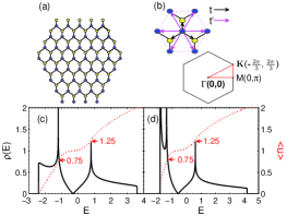
Figure 1: (Color online) (a) Sketch of graphene with double-48 sites; (b) First Brillouin zone and the high symmetry direction (red line); (c) DOS (solid dark lines ) and fillings $\langle n\rangle$ (dash red lines ) as functions of energy with $t^{\prime}$=0.10t; and (d) $t^{\prime}$=0.20t.

Our main numerical calculations were performed on a double-48 sites lattice, as sketched in Fig. 1, where blue circles and yellow circles indicates A and B sublattices, respectively. The structure of the honeycomb lattice leads to the well known massless-Dirac-fermion-like low energy excitations and the two VHS in the DOS (marked in Fig. 1) at $<$$n$$>$=0.75 and 1.25 corresponding to $E$=$-2t^{\prime}\pm t$, respectively as $t^{\prime}<t/6$. While when $t^{\prime}\geq t/6$, a third VHS appears at the lower band edge, which is a square root singularity marking the flattening of the energy band near $\Gamma$ point. They determine much of system’s properties. According to the values of $t$ and $U$ reported in the literatures for grapheneRmp ; U1 ; U2 , the ratio $U$/$\mid$t$\mid$ maybe expected to be $2.2\sim 6.0$, which is around the range of half-bandwidth to bandwidthbandwidth , where the mean filed theory does not work well while the DQMC simulation is a useful tool Hirsch . The exact value of $t^{\prime}$ is not known but an ab initio calculation Retal02 found that $t^{\prime}/t$ ranges from 0.02 to 0.2 depending on the tight-binding parameterizations. Therefore, it is necessary to study the ferromagnetic fluctuations within the Hubbard model on the honeycomb lattice by including $t^{\prime}$.

In the followings, we show that the behaviors of magnetic correlation are qualitatively different in two filling regions separated by the VHS at $<$$n$$>$=0.75. In the filling region below the VHS the system shows a short-ranged ferromagnetic correlation and the on-site Coulomb interaction tends to strengthen ferromagnetic fluctuation. The ferromagnetic properties depend on the electron filling, which may be manipulated by the electric gate. Furthermore, the ferromagnetic fluctuation is strengthened markedly as $t^{\prime}$ increases. Our results highlight the crucial importance of electron filling and the NNN hopping in graphene. The resultant controllability of FM may facilitate the new development of spintronics and quantum modulation.

To study ferromagnetic fluctuations, we define the spin susceptibility in the $z$ direction at zero frequency,

$$\chi(q)=\int_{0}^{\beta}d\tau\sum_{d,d^{\prime}=a,b}\sum_{i,j}e^{iq\cdot(i_{d}-j_{d^{\prime}})}\langle\textrm{m}_{i_{d}}(\tau)\cdot\textrm{m}_{j_{d^{\prime}}}(0)\rangle$$ (2)

where $m_{i_{a}}(\tau)$=$e^{H\tau}m_{i_{a}}(0)e^{-H\tau}$ with $m_{i_{a}}$=$a^{{\dagger}}_{i\uparrow}a_{i\uparrow}-a^{{\dagger}}_{i\downarrow}a_{i\downarrow}$ and $m_{i_{b}}$=$b^{{\dagger}}_{i\uparrow}b_{i\uparrow}-b^{{\dagger}}_{i\downarrow}b_{i\downarrow}$. Here $\chi$ is measured in unit of $\mid$$t$$\mid$^-1, and $\chi(\Gamma)$ measures ferromagnetic correlation while $\chi(K)$ measures antiferromagnetic correlation.

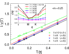
Figure 2: (Color online) At $<$$n$$>$=0.25, inverse of magnetic susceptibility, $1/\chi(q$=$\Gamma)$ versus temperature with $U$=3$\mid$t$\mid$, $t^{\prime}$=$t/10$, $t/6$, and $t/5$. Fitted line $1/\chi(\Gamma)$=$\alpha$($T-\Theta$) are also shown. Inset: Magnetic susceptibility $\chi(q)$ versus $q$ at different temperatures with $t^{\prime}$=0.10$t$ and $U$=3$\mid$$t$$\mid$.

We first present temperature dependence of the magnetic correlations at $<$$n$$>$=0.25 with different $t^{\prime}$ and $U$. Fig. 2 shows $1/\chi(q$=$\Gamma)$ versus temperature at $U$=3$\mid$$t$$\mid$ with $t^{\prime}$=$t/10$, $t/6$, and $t/5$. Data for $U$=5$\mid$$t$$\mid$ as $t^{\prime}$=$t/5$ are also shown. In the inset, we present $\chi(q)$ versus momentum $q$ at different temperatures with $t^{\prime}$=$t/10$ and $U$=3$\mid$t$\mid$. It is obvious that $\chi(q)$ has strong temperature dependence and one observes that $\chi(M)$ and $\chi(K)$ grow much slower than $\chi(\Gamma)$ with decreasing temperatures. Moreover, $1/\chi(\Gamma)$ exhibits Curie-like behavior as temperature decreases from $\mid$$t$$\mid$ to about 0.1$\mid$$t$$\mid$. Fitting the data as $1/\chi(\Gamma)$=$\alpha$($T-\Theta$) (solid lines in Fig.2) shows that $\Theta$ is about 0.02$\mid$t$\mid$$\simeq 580K$ at $t^{\prime}$=$t/5$, and we also note that both $\Theta$ and $\chi(\Gamma)$ are enhanced slightly as the on-site Coulomb interaction is increased. Positive values of $\Theta$ indicate that the curves of $1/\chi(\Gamma)$ start to bend at some low temperatures and probably converge to zero as $T\rightarrow 0$, $i.e.$, $\chi(\Gamma)$ diverges. This demonstrates the existence of ferromagnetic state in graphene.

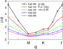
Figure 3: (Color online) Magnetic susceptibility $\chi(q)$ versus momentum $q$ at different $t^{\prime}$, here $U$=3 $\mid$t$\mid$, $<$$n$$>$=0.25 and $T$=0.10$\mid$t$\mid$.

From Fig. 2, we may also notice that $t^{\prime}$ plays a remarkable effect on the behavior of $\chi(q)$, and results for $\chi(q)$ dependent on $q$ with different $t^{\prime}$ at $U$=3$\mid$$t$$\mid$, $T$=0.10$\mid$$t$$\mid$ and $<$$n$$>$=0.25 have been shown in Fig. 3. Clearly, $\chi(\Gamma)$ gets enhanced greatly as $t^{\prime}$ increases, while $\chi(M)$ and $\chi(K)$ increase only slightly. Thus, again it is significant to demonstrate that ferromagnetic fluctuation gets enhanced markedly as $t^{\prime}$ increases. Furthermore, the strong dependence of FM on $t^{\prime}$ suggests controllability of FM in graphene by tuning $t^{\prime}$.

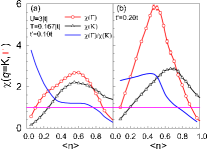
Figure 4: (Color online) Magnetic susceptibility $\chi$($q$=$\Gamma$) (red) and $\chi$($q$=$K$) (dark) versus electron filling at $U$=3$\mid$t$\mid$ and $T$=0.167$\mid$t$\mid$ with (a) $t^{\prime}$=0.1$t$ and (b) $t^{\prime}$=0.2$t$.

A great deal of current activity in graphene arises from its technological significance as a semiconductor material where carrier density can be controlled by an external gate voltageNovoselov ; Filling ; VHS . To understand filling dependence of magnetic correlations intuitively, we present $\chi(\Gamma)$ (red), $\chi(K)$ (dark), and their ratio $\chi(\Gamma)/\chi(K)$ (blue) versus filling for (a) $t^{\prime}$=0.1$t$ and (b) $t^{\prime}$=0.2$t$ in Fig. 4, where $U$=3$\mid$$t$$\mid$ and $T$=0.167$\mid$$t$$\mid$. There is a crossover between $\chi$($\Gamma$) and $\chi$($K$), which indicates that the behaviors of $\chi$($q$) are qualitatively different in two filling regions separated by the VHS at $<$$n$$>$=0.75, where the ratio is 1. This is due to the competition between ferromagnetic and antiferromagnetic fluctuations. The antiferromagnetic correlations are strong around the hall-filing and they may dominate the shape of $\chi$($q$) in a wide filling range up to the VHS. The effect of $t^{\prime}$ in enhancing ferromagnetic fluctuation can also be seen by comparing Fig. 4 (a) with (b). At electron filling $<$$n$$>$=0.25, the ratio of $\chi(\Gamma)/\chi(K)$ is about maximum for $t^{\prime}$=0.2$t$ and is substantial for $t^{\prime}$=0.1$t$, which is the reason why did we choose electron filling 0.25 in Figs. 2, and 3. From the global picture shown in Fig. 4, it is clear that the strength of ferromagnetic correlation strongly depends on the electron filling, which may be manipulated by the electric gates in graphene, since $n\propto V_{g}$Novoselov ; Filling ; VHS . The filling region for inducing FM required here likely exceeds the current experimental ability. In fact, the challenge of increasing the carrier concentration in graphene is indeed very important and it is a topic now in progress. The second gate (from the top) and/or chemical doping methods are devoted to achieving higher carrier densitybgate . Moreover, our results present here indicate the electron filling markedly affects the magnetic properties of graphene, and the controllability of FM may be realized in ferromagnetic graphene-based samples. Furthermore, the change of ferromagnetic correlation with $t^{\prime}$ may also lead to controllability of FM in graphene. For example, one can tune $t^{\prime}$ by varying the spacing between lattice sites. Tuning $t^{\prime}$ can also be realized in two sub triangular optical latticesZhu2007 ; Wu2007 . Due to the peculiar structure of graphene, which can be described in terms of two interpenetrating triangular sublattices, making controlling $t^{\prime}$ in principle possible in ultracold atoms system by using three beams of separate laserRuostekoski2009 .

In summary, we have presented exact numerical results on the magnetic correlation in the Hubbard model on a honeycomb lattice. At temperatures where the DQMC were performed, we found ferromagnetic fluctuation dominates in the low electron filling region, and it is slightly strengthened as interaction $U$ increases. The ferromagnetic correlation showed strong dependence on the electron filling and the NNN hoping integral. This provides a route to manipulate FM in ferromagnetic graphene-based samples by the electric gate or varying lattice parameters. The resultant controllability of FM in ferromagnetic graphene-based samples may facilitate the development of many applications.

The authors are grateful to Shi-Jian Gu, Guo-Cai Liu, Wu-Ming Liu and Shi-Quan Su for helpful discussions. This work is supported by HKSAR RGC Project No. CUHK 401806 and CUHK 402310. Z.B.H was supported by NSFC Grant No. 10674043.

References

- (1) S. A. Wolf, D. D. Awschalom, R. A. Buhrman, J. M. Daughton, S. von Molnr, M. L. Roukes, A. Y. Chtchelkanova, and D. M. Treger, Science 294, 1488 (2001); K. Ando, Science 312, 1883 (2006).
- (2) A. T. Hanbicki, O. M. J. vant Erve, R. Magno, G. Kioseoglou, C. H. Li, B. T. Jonker, G. Itskos, R. Mallory, M. Yasar, and A. Petrou, Appl. Phys. Lett. 82, 4092 (2003); A. Murayama, M. Sakuma, Appl. Phys. Lett., 88 122504(2006).
- (3) I. Žutić, J. Fabian and S. Das Sarma, Rev. Mod. Phys. 76, 323 (2004).
- (4) M. Dragoman and D. Dragoman, : , 2nd ed. (Artech House, Boston, 2009), Chap. 4.
- (5) A. K. Geim and K. S. Novoselov, Nat. Mater. 6, 183 (2007).
- (6) Xi Chen, Jia-Wei Tao, Appl. Phys. Lett. 94, 262102 (2009).
- (7) Y. B. Zhang, T.-T. Tang, C. Girit, Z. Hao, M. C. Martin, A. Zettl, M. F. Crommie, Y. R. Shen and F. Wang, Nature 459, 820 (2009).
- (8) Y. B. Zhang, Y.-W. Tan, H. L. Stormer and P. Kim, Nature 438, 201 (2005).
- (9) G. H. Li, A. Luican, J. M. B. Lopes dos Santos, A. H. Castro Neto, A. Reina, J. Kong and E. Y. Andrei, Nature physics 6, 109 (2010).
- (10) F. Schedin, A. K. Geim, S. V. Morozov, E. W. Hill, P. Blake, M. I. Katsnelson and K.S. Novoselov, Nature Materials 6, 652 (2007); A. Das, S. Pisana, B. Chakraborty, S. Piscanec, S. K. Saha, U. V. Waghmare, K. S. Novoselov, H. R. Krishnamurthy, A. K. Geim, A. C. Ferrari and A. K. Sood, Nature Nanotechnology 3, 210 (2008).
- (11) C. L. Kane and E. J. Mele, Phys. Rev. Lett. 95, 226801 (2005).
- (12) N. Tombros, C. Jozsa, M. Popinciuc, H.T. Jonkman and Bart J. van Wees, Nature 448, 571 (2007).
- (13) Y. B. Zhang, J. P. Small, M. E. S. Amori, and P. Kim, Phys. Rev. Lett 94, 176803 (2005); E. H. Hwang and S. Das Sarma Phys. Rev. B 77, 081412(R) (2008).
- (14) Y. Jiang, D. X. Yao, E. W. Carlson, H. D. Chen, J. P. Hu, Phys. Rev. B 77, 235420 (2008).
- (15) D. S. L. Abergel and T. Chakraborty, Phys. Rev. Lett 102, 056807 (2009).
- (16) R. Hlubina, S. Sorella, and F. Guinea, Phys. Rev. Lett. 78, 1343 (1997).
- (17) S. Q. Su, Z. B. Huang, and H. Q. Lin, J. App. Phys 103, 07C717 (2008).
- (18) N. M. R. Peres, M. A. N. Araujo, and Daniel Bozi, Phys. Rev. B 70, 195122 (2004).
- (19) T. Paiva, R. T. Scalettar, W. Zheng, R. R. P. Singh, and J. Oitmaa, Phys. Rev. B 72, 085123 (2005); N. M. R. Peres, F. Guinea, and A. H. Castro Neto, Phys. Rev. B 73, 125411 (2006).
- (20) A. H. Castro Neto, F. Guinea, N. M. R. Peres, K. S. Novoselov and A. K. Geim, Rev. Mod. Phys, 81, 109 (2009).
- (21) R. Blankenbecler, D. J. Scalapino, and R. L. Sugar, Phys. Rev. D 24, 2278 (1981).
- (22) J. E. Hirsch, Phys. Rev. B 31, 4403 (1985).
- (23) T. A. Gloor and F. Mila, Eur. Phys. J. B 38, 9 (2004); Igor F. Herbut, Phys. Rev. Lett 97, 146401 (2006).
- (24) D. Baeriswyl, D. K. Campbell, and S. Mazumdar, Phys. Rev. Lett. 56, 1509 (1986).
- (25) The bandwidth =6 when 1/6, and if 1/6, =[9++3].
- (26) S. Reich, J. Maultzsch, C. Thomsen, and P. Ordejón, Phys. Rev. B 66, 035412 (2002).
- (27) S.-L. Zhu, B.G. Wang, and L.-M. Duan, Phys. Rev. Lett. 98, 260402 (2007).
- (28) C. J. Wu, D. Bergman, L. Balents, and S. Das Sarma, Phys. Rev. Lett. 99, 070401 (2007).
- (29) J. Ruostekoski, Phys. Rev. Lett. 103, 080406 (2009); E. J. Mueller, Phys. Rev. A 70, 041603(R) (2004).