Deep inelastic scattering off a plasma with flavour from D3-D7 brane model

Abstract

We investigate the propagation of a space-like flavour current in a strongly coupled ${\cal N}=2$ super Yang-Mills plasma using the D3-D7 brane model at finite temperature. The partonic contribution to the plasma structure functions is obtained from the imaginary part of the retarded current-current commutator. At high temperatures we find a non-vanishing result, for a high energy current, indicating absorption of the flavour current by the quark constituents of the plasma. At low temperatures there is no quark contribution to the plasma structure functions.

I Introduction

Originally it was thought that the product of a heavy ion collision, the so called quark gluon plasma, would be a weakly interacting system, behaving approximately like an ideal gas. However, the experimental results from RHIC indicated that the hadronic matter formed after the collisions is strongly interacting, more similar to a perfect liquid Shuryak:2003xe . One expects an improvement in the understanding of the quark gluon plasma properties when heavy ion collisions are further investigated in the LHC.

Strong interactions are described by QCD. However, in a strong coupling regime, as the one found in the quark gluon plasma, its is necessary to use non-perturbative tools. A very interesting approach relies on the AdS/CFT correspondence which relates string theory to superconformal gauge theories at large ’t Hooft coupling. A particular case of this correspondence is given by string theory in $AdS_{5}\times S^{5}$ which is dual to ${\cal N}=4\,\,$ $SU(N_{c})$ super Yang Mills theory in four dimensions Maldacena:1997re ; Gubser:1998bc ; Witten:1998qj . This exact correspondence inspired many interesting phenomenological models known as AdS/QCD that approximately describe important aspects of hadronic physics. One of the simplest models, now called hard wall model, consists in breaking conformal invariance by introducing a hard cut off in the AdS space. The position of this cut off is related to an infrared mass scale in the dual gauge theory. The hard wall model was very successful in reproducing the scaling of hadronic scattering amplitudes at fixed angles Polchinski:2001tt ; BoschiFilho:2002zs and estimating hadronic masses BoschiFilho:2002ta ; BoschiFilho:2002vd ; deTeramond:2005su ; Erlich:2005qh ; DaRold:2005zs ; BoschiFilho:2005yh .

A more sophisticated proposal is the D3-D7 brane model that consists in the inclusion of $N_{f}$ flavoured D7 probe branes in the $AdS_{5}\times S^{5}$ space Karch:2002sh . The AdS/CFT correspondence contains fields in the adjoint representation of the $SU(N_{c})$ gauge group, like gluons, related to open strings attached to the D3 branes. Including D7 branes one also has fields in the fundamental representation, like quarks, related to open strings with an endpoint on a D3 and the other on a D7 brane. On the other side, mesons are described by strings with both endpoints on D7 branes. Masses for mesons in this model were calculated in Kruczenski:2003be . For a review see Erdmenger:2007cm .

The internal structure of hadrons can be probed by interaction processes. One is the deep inelastic scattering (DIS), that was investigated using gauge/string duality in Polchinski:2002jw ; BallonBayona:2007qr ; Hatta:2007he ; BallonBayona:2007rs ; Cornalba:2008sp ; Pire:2008zf ; Albacete:2008ze ; Gao:2009ze ; Hatta:2009ra ; BallonBayona:2008zi ; Cornalba:2009ax . Elastic form factors also give information about the hadronic structure. Form factors in AdS/QCD models were studied for example in Hong:2003jm ; Grigoryan:2007vg ; Grigoryan:2007my ; Brodsky:2007hb ; Kwee:2007nq ; RodriguezGomez:2008zp ; Bayona:2009ar . Other aspects of hadronic interaction processes using AdS/QCD have been discussed in, for example Hatta:2008tx ; Hatta:2008tn ; Hatta:2008qx ; Vega:2009zb .

The AdS/CFT correspondence can be extended to describe gauge theories at finite temperature introducing a black hole in the AdS geometry Witten:1998zw ; Son:2002sd ; Kovtun:2005ev . This version of the correspondence describes the strongly coupled ${\cal N}=4$ super Yang Mills plasma, since the particles are in a deconfined phase. The structure of this plasma was investigated in Hatta:2007cs considering a DIS process of an ${\cal R}$ current. The gravity dual of this current is a gauge field propagating in the black hole AdS space. It was found that at high energies, the ${\cal R}$ current probes the partonic behaviour of the plasma (associated with gluons), giving non-vanishing structure functions. The fact that this result occurs at any non-zero temperature is consistent with the non-confining character of the AdS-black hole model.

In this article we are going to study the structure of a strongly coupled plasma containing flavour degrees of freedom using the D3-D7 brane model at finite temperature. This consists in the inclusion of $N_{f}$ coincident D7 probe branes in the black hole AdS space Babington:2003vm ; Mateos:2006nu ; Hoyos:2006gb ; Mateos:2007vn . We consider the propagation of a space-like gauge field living in the D7 branes, corresponding to the DIS of a flavour current in a strongly coupled ${\cal N}=2$ super Yang-Mills plasma. There are two different thermal phases in the D3-D7 model: the low temperature Minkowski embedding when the D7 branes do not touch the horizon and the high temperature black hole embedding when the D7 branes have an induced horizon. We calculate in both phases the quark contribution to the plasma structure functions, considering the absorption of a flavour current by the quark constituents of the plasma. We find non-vanishing results in the high temperature phase for a high energy current. In the low temperature regime, corresponding to the Minkowski embedding, we find that the flavour current is not absorbed by the quark constituents of the plasma.

Note that the D3-D7 model contains both the $\cal R$ and flavour currents. The ${\cal R}$ current is dual to a gauge field propagating in the bulk geometry generated by the D3 branes while the flavour current dual is a gauge field propagating on the world volume of the D7 branes. This way, studying a DIS process in this model we can unveil not only the partonic structure associated with gluons but also the partonic structure associated with quarks.

This article is organized as follows. In section II, we briefly review the ${\cal R}$ current results. Then, we study, in section III, the equations of motion of a gauge field on the D7 branes. In section IV we analyse the effective potentials at low and high temperatures and calculate the quark contribution to the plasma structure functions in these regimes. We end, in section V, with our conclusions.

II Deep inelastic scattering of an ${\cal R}$ current

In this section we briefly review the calculation of the retarded current-current correlator of an ${\cal R}$ current and the corresponding DIS structure functions. According to the AdS/CFT correspondence at finite temperature, an ${\cal N}=4$ super Yang Mills $SU(N_{c})$ plasma is dual to a black hole in $AdS_{5}\times S^{5}$ space. This space can be described by the metric

$$ds^{2}\,=\,\frac{r_{0}^{2}}{L^{2}u}\Big{[}-(1-u^{2})dt^{2}\,+\,d{\bar{x}}^{2}\Big{]}\,+\,\frac{L^{2}}{4u^{2}(1-u^{2})}du^{2}\,+\,L^{2}d\Omega^{2}_{5}\,,$$ (1)

where $r_{0}\,=\,\pi L^{2}T$ ,   $L$ is the AdS radius ($L^{4}\,=\,4\pi\alpha^{\prime 2}g_{YM}^{2}N_{c}$),   $T$ is the temperature and $d\Omega^{2}_{5}$ is the $S^{5}$ metric. The radial coordinate $u$ is dimensionless, with the horizon located at $u=1$ and the boundary at $u=0$.

The vector field $A_{m}=(A_{u},A_{\mu})$ dual to the ${\cal R}$-current is described by the supergravity action

$$S\,=\,-\,\frac{N_{c}^{2}}{64\pi^{2}L}\int d^{4}xdu\sqrt{-g}\,g^{mr}g^{ns}\,F_{mn}F_{rs}\,\,.$$ (2)

Choosing the gauge $A_{u}=0$ and the plane wave solution

$$A_{\mu}(x,u)\,=\,e^{-iq\cdot x}{\bar{A}}_{\mu}(u)\,\,,$$ (3)

with $q^{\mu}=(w,0,0,q)$, the on shell action takes the form

$$S\,=\,-\,\frac{N_{c}^{2}T^{2}}{16}\int d^{4}x\Big{[}\Big{(}A_{t}+\frac{{\bar{w}}}{\bar{q}}A_{3}\Big{)}\,\partial_{u}A_{t}\,-\,A_{i}\partial_{u}A_{i}\Big{]}_{u=0}\,\,,$$ (4)

where $i=1,2$, ${\bar{w}}\equiv\frac{w}{2\pi T}\,$ , $\,\,{\bar{q}}\equiv\frac{q}{2\pi T}\,\,$ and we used the relation $\partial_{u}A_{t}=({\bar{q}}/{\bar{w}})\partial_{u}A_{3}$ valid at the boundary $u=0$.

The retarded current-current commutator of the boundary gauge theory is defined by

$$R_{\mu\nu}(q)\,=\,i\int d^{4}x\,e^{-iq\cdot x}\,\theta(t)\langle[J_{\mu}(x),J_{\nu}(0)]\rangle$$ (5)

and can be decomposed as

$$R_{\mu\nu}\,=\,\Big{(}\eta_{\mu\nu}\,-\,\frac{q_{\mu}q_{\nu}}{Q^{2}}\,\Big{)}R_{1}\,+\,\Big{[}n_{\mu}n_{\nu}\,-\,\frac{n\cdot q}{Q^{2}}(n_{\mu}q_{\nu}+n_{\nu}q_{\mu})\,+\frac{q_{\mu}q_{\nu}}{(Q^{2})^{2}}(n\cdot q)^{2}\,\Big{]}R_{2}\,,$$ (6)

where $n^{\mu}$ is the four velocity of the plasma and $Q^{2}$ is the virtuality defined by $Q^{2}\equiv q^{2}-w^{2}$. In the plasma rest frame $n^{\mu}=(1,0,0,0)$. The DIS structure functions of the plasma are given by

$$F_{1}=\frac{1}{2\pi}{\rm Im}\,R_{1}\hskip 28.45274ptF_{2}=-\frac{n\cdot q}{2\pi T}\,{\rm Im}\,R_{2}\,.$$ (7)

These structure functions can be obtained from those of the DIS off a hadron identifying the hadronic momentum $P^{\mu}$ with the plasma momentum $Tn^{\mu}$.

Following a supergravity prescription similar to that of ref. Son:2002sd , the retarded current-current commutator is obtained by differentiating the boundary action density with respect to the boundary values of the vector fields

$$R_{\mu\nu}(q)\,=\,\frac{\partial^{2}{\cal S}}{\partial A^{(0)}_{\mu}\partial A^{(0)}_{\nu}}\;;\qquad\qquad(A^{(0)}_{\mu}=\lim_{u\to 0}A_{\mu})\;,$$ (8)

after imposing an ingoing condition for the gauge fields at the horizon, meaning that there is no reflection.

The equations of motion for the components of the gauge fields can be written as Schrödinger equations. For the longitudinal part it reads

$$\frac{\partial^{2}\psi}{\partial u^{2}}-V(u)\psi\,=\,0\,,$$ (9)

where $\psi(u)=\sqrt{u(1-u^{2})}\,\partial_{u}A_{t}\,$ and the effective potential is

$$V(u)=\frac{1}{u(1-u^{2})^{2}}\,\Big{[}-\frac{1}{4u}(1+6u^{2}-3u^{4})+{\bar{Q}}^{2}-{\bar{q}}^{2}u^{2}\Big{]}\,,$$ (10)

with ${\bar{Q}}^{2}\equiv{\bar{q}}^{2}-{\bar{w}}^{2}$. For the transversal components we have

$$\frac{\partial^{2}\phi}{\partial u^{2}}-{\tilde{V}}(u)\phi\,=\,0\,,$$ (11)

where $\phi(u)=\sqrt{(1-u^{2})}\,A_{i}(u)\,$ and

$${\tilde{V}}(u)\,=\,\frac{1}{u(1-u^{2})^{2}}\,\Big{[}{\bar{Q}}^{2}-{\bar{q}}^{2}u^{2}-u\Big{]}$$ (12)

Analysing the behaviour of the potentials (10) and (12) one finds different regimes depending on the relation between ${\bar{q}}$ and ${\bar{Q}}\,$ Hatta:2007cs . These regimes are separated by the critical value ${\bar{q}}/{\bar{Q}}^{3}=8/(3\sqrt{3})\approx 1.54$. At low energies, ${\bar{q}}/{\bar{Q}}^{3}\ll 1$, there is no relevant contribution to the structure functions since the imaginary part of $R_{\mu\nu}$ is negligible. At high energies ${\bar{q}}/{\bar{Q}}^{3}\gg 1$, a significant imaginary term arises in $R_{\mu\nu}$ leading to the non vanishing structure functions

$$F_{1} \approx \frac{3}{16\Gamma^{2}(1/3)}\,N_{c}^{2}T^{2}\left(\frac{Q^{2}}{12\pi T^{2}x}\right)^{2/3}$$

$$F_{2} \approx 2xF_{1}\,,$$ (13)

where $x$ is the Bjorken variable that in the plasma rest frame takes the form $x=Q^{2}/2wT\,$. These structure functions imply dissipation of the ${\cal R}$ current, unveiling the existence of a partonic structure associated with gluons in the ${\cal N}=4$ super Yang Mills plasma, as discussed in ref. Hatta:2007cs . Note that these results for the ${\cal R}$ current are also valid in the ${\cal N}=2$ super Yang Mills plasma of the D3-D7 brane model.

III Deep inelastic scattering of a flavour current

III.1 The D7 brane embedding

We place $N_{f}$ coincident D7 probe branes in the black hole $AdS_{5}\times S^{5}$ space of eq. (1). In order to describe the D7 probe branes, we decompose the metric of the sphere $S^{5}$ as

$$d\Omega^{2}_{5}\,=\,d\theta^{2}\,+\,\sin^{2}\theta d\Omega^{2}_{3}\,+\,\cos^{2}\theta d\varphi^{2}\,.$$ (14)

The usual choice is to fix $\varphi=0$ and $\theta=\theta(u)$. Then, each D7 brane is described by the metric

$$ds^{2}\,=\,\frac{r_{0}^{2}}{L^{2}u}\Big{[}-(1-u^{2})dt^{2}\,+\,d{\bar{x}}^{2}\Big{]}\,+\,L^{2}\Big{[}\frac{1}{4u^{2}(1-u^{2})}\,+\,\theta^{\prime 2}\Big{]}du^{2}\,+\,L^{2}\sin^{2}\theta d\Omega^{2}_{3}\,.$$ (15)

Here, and from now on, prime denotes differentiation with respect to the variable $u$. The location of the D7 branes is contained in $\theta=\theta(u)$. This function is obtained by solving the equation of motion that comes from the brane action:

$$S_{D7} \,=\, \,-\,N_{f}\,\mu_{7}\int d^{8}x\sqrt{-\det g}$$ (16)

$$\,=\, \,-\,N_{f}\,\mu_{7}\pi^{2}r_{0}^{4}\int d^{4}x\,\int_{0}^{1}\frac{du}{u^{3}}\sin^{3}\theta\sqrt{1+4u^{2}(1-u^{2})\theta^{\prime 2}}\,.$$

where $\mu_{7}\,=\,[(2\pi)^{7}g_{YM}^{2}\,\alpha^{\prime 4}]^{-1}$ is the tension of each D7 brane. The D7 brane equation of motion reads

$$3\cos\theta\Big{[}1+4u^{2}(1-u^{2})\theta^{\prime 2}\Big{]}\,+\,4u\sin\theta\Big{[}-u(1-u^{2})\theta^{\prime\prime}+4u^{2}(1-u^{2})(2-u^{2})\theta^{\prime 3}+(1+u^{2})\theta^{\prime}\Big{]}=0\,.$$ (17)

There are solutions of three different kinds. In the first one, the branes touch the black hole horizon. This solution is called black hole embedding. An observer living on the branes world volume will see an induced horizon. In the second kind of solutions the branes never reach the horizon. This solution is known as Minkowski embedding. In this case, an observer on the branes do not see any induced horizon. The third solution is a critical embedding that connects the black hole and Minkowski embeddings.

Near the boundary all the solutions have the asymptotic expansion

$$\theta(u)\,=\,\frac{\pi}{2}\,-\,\frac{m}{\sqrt{2}}u^{1/2}\,-\,\frac{1}{2\sqrt{2}}(\frac{m^{3}}{6}+c\,)u^{3/2}+...\,\,,$$ (18)

where $m\equiv M/T$ with $M$ proportional to the mass gap at zero temperature and $c$ is the quark condensate. Below we briefly review the differences between these three embeddings in the region far from the boundary and the phase transition between the Minkowski and black hole embeddings, found in Mateos:2007vn .

III.1.1 The black hole embedding

The black hole embedding is characterized by the condition that the coordinate $\theta(u)$ goes to a constant value $\theta_{0}$ different from zero at the horizon:   $\theta(1)=\theta_{0}$ .

It is convenient to use the variable $\chi(u)\equiv\cos\theta(u)$ which has the near horizon expansion

$$\chi(u)=\chi_{0}+\chi_{1}(1-u)+\chi_{2}(1-u)^{2}+\dots\,,$$ (19)

with $0\leq\chi_{0}<1$. Using this expansion in (17) we obtain

$$\chi_{1}=-\frac{3}{8}\chi_{0}\quad\rightarrow\quad\theta^{\prime}(1)=-\frac{3}{8}\cot\theta_{0}\,.$$ (20)

We use the above conditions for $\theta$ and $\theta^{\prime}$ as initial conditions at $u=1$ for the numerical integration of eq. (17).

A typical solution is illustrated on Fig. 1. As shown in Mateos:2007vn , black hole embeddings exist only for temperatures higher than $0.764M$.

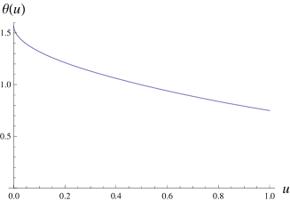
Figure 1: Black hole D7 metric for $\theta_{0}\,=\,0.75$ .

III.1.2 The Minkowski embedding

On the other hand, in the case of Minkowski embedding the coordinate $u$ has a maximum value $u_{0}<1$ where the coordinate $\theta$ vanishes: $\theta(u_{0})=0$. The region $u=u_{0}$ is interpreted as the tip of the branes. The requirement of smoothness without conical deficit at the tip of the branes leads to $\theta^{\prime}(u_{0})=-\infty$ Hoyos:2006gb .

These conditions on $\theta$ and $\theta^{\prime}$ suggest the near horizon expansion

$$\theta=\left(1-\frac{u}{u_{0}}\right)^{\alpha}\left[\rho_{0}+\rho_{1}\left(1-\frac{u}{u_{0}}\right)+\rho_{2}\left(1-\frac{u}{u_{0}}\right)^{2}+\dots\right]\,,$$ (21)

with $0<\alpha<1$.Using this expansion in (17) we obtain

$$\alpha=\frac{1}{2}\quad,\quad\rho_{0}=\sqrt{\frac{2}{2-u^{2}_{0}}}\,.$$ (22)

In the numerical integration we evaluate this asymptotic expression and its derivative at some $u$ very close (but not equal) to $u_{0}$. A typical solution is shown in Fig. 2.

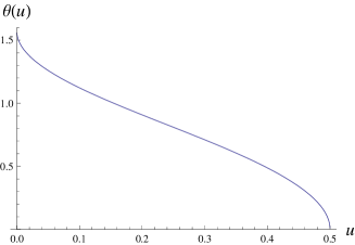
Figure 2: Minkowski D7 metric for $u_{0}\,=\,0.5$.

As shown in Mateos:2007vn , Minkowski embeddings exist only for temperatures lower than $0.772M$.

III.1.3 The critical embedding

The critical embedding appears as an intermediate solution between black hole embeddings and Minkowski embeddings. In this case the coordinate $u$ reaches the horizon when the coordinate $\theta$ goes to zero. This is shown in Fig. 3.

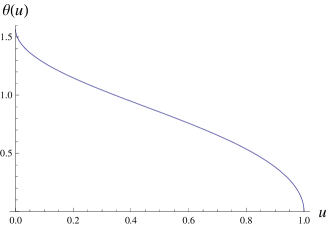
Figure 3: Critical D7 metric corresponding to $\theta_{0}\,=\,0$ or $u_{0}\,=\,1$ .

III.1.4 The phase transition

The Minkowski and black hole embeddings can coexist for temperatures between $0.764M$ and $0.772M$. However, the physical embedding is the one that minimizes the free energy at a given temperature. It was shown in Mateos:2007vn that a first order transition occurs at a temperature $T_{c}=0.766M$. Below $T_{c}$ the Minkowski embedding has the lower free energy so it is thermodynamically preferred while the black hole embedding is dominant above $T_{c}$.

A consequence of this first order phase transition is a finite jump in the quark condensate at $T=T_{c}$, where the D7 branes go from a Minkowski embedding to a black hole embedding. We will see below how the abrupt change in the D7 brane embedding has a non-trivial consequence on the partonic contribution to the structure functions of the ${\cal N}=2$ super Yang-Mills plasma when probed by a flavour current.

III.2 Gauge field equations and Schrödinger potentials

We consider a flavour current $U(1)\subset U(N_{f})$. The gravity dual of this current is a gauge field fluctuation living in the world volume of the D7 branes. From the Dirac Born Infeld action one finds the gauge field kinetic term

$$S\,=\,-\,N_{f}\mu_{7}\,\pi^{2}\alpha^{\prime 2}\int d^{8}x\sqrt{-G}\,\,F_{MN}F^{MN}\,\,,$$ (23)

where $F_{MN}=\partial_{M}A_{N}-\partial_{N}A_{M}\,$ and $A_{M}=(A_{\mu},A_{u},A_{\alpha})\,$. We choose $A_{\alpha}=0$, $\partial_{\alpha}A_{\mu}=0$, $A_{u}=0$ and the plane wave ansatz

$$A_{\mu}(x,u)\,=\,\exp\{-iwt+iqx^{3}\}\,{\bar{A}}_{\mu}(u)\,.$$ (24)

The equations of motion take the form

$$\partial_{u}A_{3} = -\,\frac{\bar{w}}{{\bar{q}}(1-u^{2})}\partial_{u}A_{t}$$ (25)

$$\frac{\Gamma^{1/2}}{\sin^{3}\theta}\partial_{u}\Big{[}\frac{\sin^{3}\theta}{\Gamma^{1/2}}\partial_{u}A_{t}\Big{]} - \frac{\Gamma}{u(1-u^{2})}\Big{[}{\bar{q}}^{2}A_{t}+{\bar{q}}{\bar{w}}A_{3}\Big{]}\,=\,0$$ (26)

$$\frac{\Gamma^{1/2}}{\sin^{3}\theta(1-u^{2})}\partial_{u}\Big{[}\frac{\sin^{3}\theta(1-u^{2})}{\Gamma^{1/2}}\partial_{u}A_{i}\Big{]} - \frac{\Gamma}{u(1-u^{2})^{2}}\Big{[}-{\bar{w}}^{2}\,+\,(1-u^{2}){\bar{q}}^{2}\Big{]}A_{i}\,=\,0\;,\;\;\;$$ (27)

where $\Gamma\equiv 1+4u^{2}(1-u^{2})\theta^{\prime 2}$  .

In order to gain intuition on the problem, we write the gauge field equations (25), (26) and (LABEL:transverseeq) into a Schrödinger form, as in ref. Myers:2007we . We will find two relevant potentials whose form determine the behavior of the retarded current-current commutator and hence the partonic contribution to the DIS structure functions.

III.2.1 Longitudinal component

Using $\,a(x,u)\equiv\partial_{u}A_{t}\,$, we find from eqs. (25) and (26) the second order differential equation

$$\partial^{2}_{u}a\,+\,\frac{1}{H_{1}}\partial_{u}H_{1}\partial_{u}a\,-\,\frac{1}{H_{0}}\Big{[}H_{3}+H_{2}\,{\bar{q}}^{2}\,-\,{\bar{w}}^{2}\,\Big{]}a\,=\,0\,,$$ (29)

where

$$H_{0} = \frac{u(1-u^{2})^{2}}{\Gamma}$$

$$H_{1} = \frac{u(1-u^{2})\sin^{3}\theta}{\Gamma^{3/2}}$$

$$H_{2} = 1-u^{2}$$

$$H_{3} = -(1-u^{2})\partial_{u}\Big{[}\frac{u-u^{3}}{\Gamma}\Big{(}3\,\cot\theta\,\,\theta^{\prime}\,-\,\frac{\Gamma^{\prime}}{2\Gamma}\Big{)}\,\Big{]}\;.$$ (30)

Introducing: $a(x,u)={\eta}(u)\psi(x,u)$ and imposing that

$$\frac{\eta^{\prime}}{\eta}=-\frac{1}{2}\frac{H_{1}^{\prime}}{H_{1}}\,,$$ (31)

we find a Schrödinger equation

$$\frac{d^{2}\psi}{du^{2}}\,-\,V(u)\,\psi\,=\,0\,,$$ (32)

with potential

$$V(u) = \frac{1}{2}\Big{(}\frac{H_{1}^{\prime}}{H_{1}}\Big{)}^{\prime}+\frac{1}{4}\Big{(}\frac{H_{1}^{\prime}}{H_{1}}\Big{)}^{2}+\,\frac{1}{H_{0}}\Big{[}H_{3}+H_{2}{\bar{q}}^{2}\,-\,{\bar{w}}^{2}\,\Big{]}$$ (33)

$$= \frac{3u^{4}-6u^{2}-1}{4u^{2}(1-u^{2})^{2}}\,+\,\frac{\Gamma}{u(1-u^{2})^{2}}\Big{[}{\bar{Q}}^{2}-u^{2}{\bar{q}}^{2}\Big{]}\,-\frac{3}{2}\cot\theta\,\theta^{\prime\prime}-\frac{\Gamma^{\prime\prime}}{4\Gamma}\,-\,\frac{\Gamma^{\prime}}{4\Gamma}\frac{1-3u^{2}}{u(1-u^{2})}$$

$$+ \frac{3}{2}\cot\theta\,\theta^{\prime}\Big{[}\frac{\Gamma^{\prime}}{2\Gamma}\,-\,\frac{1-3u^{2}}{u(1-u^{2})}\Big{]}\,+\,\frac{3}{2}\Big{(}1\,+\,\frac{5}{2}\cot^{2}\theta\Big{)}{\theta^{\prime}}^{2}\,+\,\frac{5}{16}\Big{(}\frac{\Gamma^{\prime}}{\Gamma}\Big{)}^{2}\,.$$

A possible solution to eq.(31) is ${\eta}=C(-H_{1})^{-1/2}$, with $C$ an arbitrary constant, chosen for convenience as $C\,=\,2\sqrt{2}r_{0}^{2}/L^{2}$. Near the boundary and in the Bjorken limit $\bar{Q}^{2}\gg m^{2}$, the longitudinal potential can be approximated by

$$V(u) = -\frac{1}{4u^{2}}\,+\,\frac{{\bar{Q}}^{2}}{u}\,+\frac{m^{2}}{2}{\bar{Q}}^{2}\,-{\bar{q}}^{2}u\,-\,\frac{m^{2}}{2}{\bar{q}}^{2}u^{2}\,.$$ (34)

The terms containing $m^{2}$ represent small perturbations of the near boundary approximation of the potential (10). If we consider the interesting high energy regime $\bar{q}\gg\bar{Q}^{3}$ this potential reduces to

$$V(u) = -\frac{1}{4u^{2}}\,-{\bar{q}}^{2}u\,-\,\frac{m^{2}}{2}{\bar{q}}^{2}u^{2}\,.$$ (35)

This expression will be useful for the calculation of the DIS structure functions in section IV.

III.2.2 Transversal component

In a similar way, for the transversal modes, eq. (LABEL:transverseeq) can be rewritten as

$$\partial^{2}_{u}A_{i}\,+\,\frac{1}{\tilde{H}_{1}}\partial_{u}{\tilde{H}}_{1}\partial_{u}A_{i}\,-\,\frac{1}{H_{0}}\Big{[}H_{2}\,{\bar{q}}^{2}\,-\,{\bar{w}}^{2}\,\Big{]}A_{i}\,=\,0\,,$$ (36)

where

$${\tilde{H}}_{1} = \frac{(1-u^{2})\sin^{3}\theta}{\Gamma^{1/2}}\,.$$ (37)

Defining $\,A_{i}(x,u)\,=\,\epsilon(u)\,\Phi_{i}(x,u)\,$ and imposing

$$\frac{\epsilon^{\prime}}{\epsilon}=-\frac{1}{2}\frac{{\tilde{H}_{1}^{\prime}}}{{\tilde{H}_{1}}}\,,$$ (38)

we find a Schrödinger equation for $\Phi_{i}(x,u)$, similar to eq. (32), with the potential

$$\tilde{V}(u) = \frac{1}{2}\Big{(}\frac{{\tilde{H}}_{1}^{\prime}}{{\tilde{H}}_{1}}\Big{)}^{\prime}+\frac{1}{4}\Big{(}\frac{{\tilde{H}}_{1}^{\prime}}{{\tilde{H}}_{1}}\Big{)}^{2}+\,\frac{1}{H_{0}}\Big{[}\,H_{2}{\bar{q}}^{2}\,-\,{\bar{w}}^{2}\,\Big{]}$$ (39)

$$= -\frac{1}{(1-u^{2})^{2}}\,+\,\frac{\Gamma}{u(1-u^{2})^{2}}\Big{[}{\bar{Q}}^{2}-u^{2}{\bar{q}}^{2}\Big{]}\,+\frac{3}{2}\cot\theta\,\theta^{\prime\prime}-\frac{\Gamma^{\prime\prime}}{4\Gamma}\,+\,\frac{u}{(1-u^{2})}\frac{\Gamma^{\prime}}{2\Gamma}$$

$$- \frac{3}{2}\cot\theta\,\theta^{\prime}\Big{[}\frac{\Gamma^{\prime}}{2\Gamma}\,+\,\frac{2u}{(1-u^{2})}\Big{]}\,+\,\frac{3}{2}\Big{(}-1\,+\,\frac{1}{2}\cot^{2}\theta\Big{)}{\theta^{\prime}}^{2}\,+\,\frac{5}{16}\Big{(}\frac{\Gamma^{\prime}}{\Gamma}\Big{)}^{2}\,.$$

The solution to eq. (38) is $\epsilon\,=\,\tilde{C}(\tilde{H}_{1})^{-1/2}$ and we choose for convenience $\tilde{C}\,=\,\sqrt{2}r_{0}$. Again, near the boundary and for $\bar{Q}^{2}\gg m^{2}$, we find the approximate transversal potential

$${\tilde{V}}(u) = \frac{{\bar{Q}}^{2}}{u}\,+\frac{m^{2}}{2}{\bar{Q}}^{2}\,-{\bar{q}}^{2}u\,-\,\frac{m^{2}}{2}{\bar{q}}^{2}u^{2}\,.$$ (40)

In the high energy regime $\bar{q}\gg\bar{Q}^{3}$ this potential can be approximated by

$${\tilde{V}}(u) = -{\bar{q}}^{2}u\,-\,\frac{m^{2}}{2}{\bar{q}}^{2}u^{2}\,.$$ (41)

III.3 The retarded flavour current commutator

The on-shell action for the gauge field has the following boundary term

$$S_{B}\,=\,8\pi^{4}\alpha^{\prime 2}\,N_{f}\,\mu_{7}\,\,r_{0}^{2}\left\{\frac{\sin^{3}\theta}{\Gamma^{1/2}}\int d^{4}x[\,-(A_{t}+\frac{\bar{w}}{\bar{q}}A_{3})\,a+(1-u^{2})A_{i}\partial_{u}A_{i}]\right\}_{u=0},$$ (42)

where $i=1,2$. The hypersurface $u=0$ defines the boundary which excludes the horizon or the tip of the D7 branes.

We will use this boundary action to calculate the quark contribution to the plasma structure functions. The near boundary expansions for the fields $a$ and $A_{i}$ that satisfy the equations of motion are given by

$$a(x,u) \,=\, \bar{q}^{2}\left[A^{(0)}_{t}+\frac{\bar{w}}{\bar{q}}A^{(0)}_{3}\right]\,\left\{a_{0}\,+\,\ln{u}\,+\,a_{1}u\,+\,b_{1}u\ln{u}\,+\,{\cal O}(u^{2})\,+\,{\cal O}(u^{2}\ln{u})\right\}$$

$$A_{i}(x,u) \,=\, A^{(0)}_{i}\left\{1\,+\,\bar{Q}^{2}[c_{1}u\,+\,d_{1}u\ln{u}]\,+\,{\cal O}(u^{2})\,+\,{\cal O}(u^{2}\ln{u})\right\}$$ (43)

where $A^{(0)}_{\mu}(x)\,=\,A_{\mu}(x,u)|_{{}_{u=0}}$. The coefficients $a_{0},\,a_{1},\,b_{1},\,c_{1},\,,d_{1}$ can be obtained from the differential equations (29) and (36). With these expansions the boundary on shell action can be written as

$$S_{B}\,=\,\frac{N_{f}N_{c}}{16\pi^{2}}\,\int d^{4}x\Big{\{}\,-q^{2}\,[A^{(0)}_{t}+\frac{\bar{w}}{\bar{q}}A^{(0)}_{3}]^{2}\,(\,\ln{u}+a_{0}\,)\,$$

$$+\,Q^{2}A^{(0)}_{i}A^{(0)}_{i}\,(\,d_{1}\ln{u}+c_{1}+d_{1}\,)\Big{\}}_{u=0}\,,$$ (44)

The divergent logarithmic terms can be canceled by the following (boundary) counterterms

$$S_{ct}\,=\,\frac{N_{f}N_{c}}{16\pi^{2}}\,\int d^{4}x\Big{\{}\,q^{2}\,[A^{(0)}_{t}+\frac{\bar{w}}{\bar{q}}A^{(0)}_{3}]^{2}\,\left[\,\ln{u}+2\gamma+2\ln{(\frac{M}{2\pi T})}\right]\,$$

$$-\,Q^{2}\,A^{(0)}_{i}A^{(0)}_{i}\,d_{1}\,\left[\ln{u}+2\gamma+2\ln{(\frac{M}{2\pi T})}\right]\Big{\}}_{u=0}\,,$$ (45)

where we have included in the counterterms the temperature $T$ and the infrared scale $M$ is the D7 brane mass scale at zero temperature defined in the previous section. We also included the Euler-Mascheroni constant $\gamma$ as is done in Hatta:2007cs . Summing both terms we obtain the total finite action

$$S_{Total} = \frac{N_{f}N_{c}}{16\pi^{2}}\,\int d^{4}x\Big{\{}\,\left(\eta_{\mu\nu}-\frac{q_{\mu}q_{\nu}}{Q^{2}}\right)Q^{2}\,\left[\,c_{1}+d_{1}-2\gamma\,d_{1}-2\ln{(\frac{M}{2\pi T})}\,d_{1}\right]$$ (46)

$$+ (n_{\mu}-q_{\mu}\frac{n\cdot q}{Q^{2}})(n_{\nu}-q_{\nu}\frac{n\cdot q}{Q^{2}})\,\frac{Q^{4}}{q^{2}}\left[c_{1}+d_{1}-a_{0}+2\ln{(\frac{M}{2\pi T})}(1-d_{1})+2\gamma(1-d_{1})\right]\Big{\}}$$

$$\times A^{(0)\mu}A^{(0)\nu}$$

So, differentiating this action with respect to the boundary values of the gauge fields, as in eq. (8), we obtain

$$R_{1}(q,Q^{2}) \,=\, \frac{N_{f}N_{c}}{8\pi^{2}}Q^{2}\,\left[c_{1}+d_{1}\left[1-2\gamma\,-2\ln{(\frac{M}{2\pi T})}\right]\right]$$ (47)

$$R_{2}(q,Q^{2}) \,=\, \frac{N_{f}N_{c}}{8\pi^{2}}\,\frac{Q^{4}}{q^{2}}\left[c_{1}+d_{1}-a_{0}+(1-d_{1})\left[2\ln{(\frac{M}{2\pi T})}+2\gamma\right]\right]\,.$$ (48)

We end this section writing the near boundary expansion for the longitudinal and transversal wave functions

$$\psi(x,u) \,=\, \bar{q}^{2}\left[A^{(0)}_{t}+\frac{\bar{w}}{\bar{q}}A^{(0)}_{3}\right]\,u^{1/2}\,\Big{\{}a_{0}\,+\,\ln{u}\,+\,(a_{1}-\frac{m^{2}}{2}a_{0})u\,+\,(b_{1}-\frac{m^{2}}{2})u\ln{u}$$ (49)

$$\,+\, {\cal O}(u^{2})\,+\,{\cal O}(u^{2}\ln{u})\Big{\}}$$

$$\Phi_{i}(x,u) \,=\, A^{(0)}_{i}\left\{1\,+\,(\bar{Q}^{2}c_{1}-\frac{m^{2}}{4})u\,+\,\bar{Q}^{2}d_{1}u\ln{u}\,+\,{\cal O}(u^{2})\,+\,{\cal O}(u^{2}\ln{u})\right\}$$ (50)

that are obtained from eqs. (43). These expansions will be useful in the analysis of the next section.

IV Structure functions

In the case of an ${\cal R}$ current there is a transition between hadronic and partonic behavior, when going from low to high energies, as discussed in section II. The partonic behaviour is characterized by non vanishing structure functions. This transition corresponds also to a change in the shape of the longitudinal and transversal potentials. At low energies, both potentials present barriers that prevent wave propagation from the boundary to the horizon. When increasing the energy the longitudinal potential barrier disappears while the transversal potential gets squeezed towards the boundary so that the wave propagates into the black hole and is absorbed by the horizon.

For the flavour current, the scenario is substantially different because the D7 brane geometry changes drastically with temperature. For temperatures lower than $0.766M$ the D7 branes, where the gauge field lives, do not touch the horizon (Minkowski embedding) while for temperatures higher than $0.766M$ they have an induced horizon (black hole embedding). We now analyse the effective potentials in these two cases.

IV.1 Low temperatures: Minkowski embedding

At temperatures lower than $T_{c}=0.766M$, the thermodynamically preferred D7 brane solution is the Minkowski embedding. In this embedding, the radial coordinate $u$ never touches the black hole horizon. This coordinate has a maximum value $u_{0}$ where the tip of the D7 branes is localized. This geometric constraint has to be present when studying the dynamics of gauge field fluctuations. In fact, the ending condition of the radial coordinate emerges in the potential. This is illustrated in figures 4 - 7 where we plot longitudinal and transversal flavour current potentials for different energy regimes compared with the corresponding ${\cal R}$ current potentials. One can see that near the boundary the flavour current potentials behave in a similar way as the ${\cal R}$ current potentials. However, near the tip of the branes the flavour current potentials present an infinite barrier forbidding the wave to reach the black hole horizon. In contrast, the ${\cal R}$ current potentials go smoothly to the horizon.

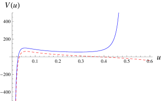
Figure 4: Low temperature and low energy ($\bar{q}\,=\,0.3\bar{Q}^{3}$) longitudinal potential of a flavour current (solid line) with $u_{0}\,=\,0.5$, compared to that of an ${\cal R}$ current (dashed line).

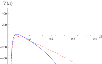
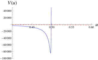
Figure 5: Low temperature and high energy ($\bar{q}\,=\,1.6\bar{Q}^{3}$) longitudinal potential of a flavour current (solid line) with $u_{0}\,=\,0.5$, compared to that of an ${\cal R}$ current (dashed line). The left (right) panel corresponds to small (large) $u$.

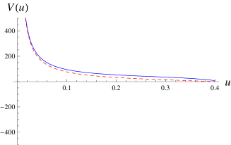
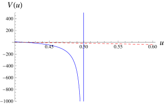
Figure 6: Low temperature and low energy ($\bar{q}\,=\,0.3\bar{Q}^{3}$) transversal potential of a flavour current (solid line) with $u_{0}\,=\,0.5$, compared to that of an ${\cal R}$ current (dashed line). The left (right) panel corresponds to small (large) $u$.

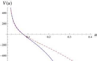
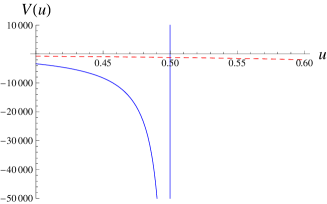
Figure 7: Low temperature and high energy ($\bar{q}\,=\,1.6\bar{Q}^{3}$) transversal potential of a flavour current (solid line) with $u_{0}\,=\,0.5$, compared to that of an ${\cal R}$ current (dashed line). The left (right) panel corresponds to small (large) $u$.

In the Minkowski embedding, the branes do not touch the horizon. Therefore, one can not impose ingoing boundary conditions for the wave functions. This can be seen by considering the asymptotic expansion of the longitudinal and transversal fields

$$a(x,u) = \left(1-\frac{u}{u_{0}}\right)^{\alpha}\left[\tilde{a}_{0}+\tilde{a}_{1}\left(1-\frac{u}{u_{0}}\right)+\tilde{a}_{2}\left(1-\frac{u}{u_{0}}\right)^{2}+\dots\right]$$ (51)

$$A_{i}(x,u) = \left(1-\frac{u}{u_{0}}\right)^{\beta}\left[\tilde{A}_{i,0}+\tilde{A}_{i,1}\left(1-\frac{u}{u_{0}}\right)+\tilde{A}_{i,2}\left(1-\frac{u}{u_{0}}\right)^{2}+\dots\right]\,.$$ (52)

Using these expansions in eqs. (29) and (36) we obtain the conditions

$$\alpha(\alpha+2)=0\quad,\quad\beta(\beta+1)=0\,.$$ (53)

with real solutions $\alpha=(0,-2)$ and $\beta=(0,-1)$. Then, the longitudinal and transversal gauge fields behave as real functions near the tip of the D7 branes, as well as on the boundary. So, these solutions are not compatible with an ingoing condition. Instead, we impose regularity of these solutions at the tip of the branes, that corresponds to $\alpha=0$ and $\beta=0$.

This way, the infinite barrier inhibits the gravitational wave to reach the horizon. The wave is not absorbed but reflected at the tip of the branes, leading to stationary real solutions. As a consequence, the coefficients arising in the near boundary expansion of the longitudinal and transversal wave functions , eqs. (49) and (50), are also real, as well as $R_{1}$ and $R_{2}$, given by eqs. (47) and (48). This translates into the vanishing of the quark contribution to the structure functions $F_{1}$ and $F_{2}$. Since the infinite barriers in the effective potentials exist at any energy scale, we conclude that the strongly coupled plasma does not show partonic behaviour when interacting with a flavour current at temperatures below $T_{c}$. This result contrasts with the case of an ${\cal R}$ current at high energy, that indicates a partonic behaviour (associated with gluons) at any temperature.

IV.2 High temperatures: black hole embedding

At temperatures above $T_{c}=0.766M$, the thermodynamically dominant solution is the black hole D7 embedding where the D7 branes touch the horizon. In this case, the gauge field waves can be absorbed by the black hole horizon, depending on the shape of the effective potentials. These potentials vary with the momentum scales $\bar{q}\,$ and $\bar{Q}$ and also with the D7 brane parameter $m$ (mass scale).

The form of the potentials is determined essentially by the ratio ${\bar{q}}/{\bar{Q}}^{3}$. In the low energy case $\bar{q}\,\ll\,\bar{Q}^{3}$ the potentials present large barriers that inhibit propagation towards the horizon. This is illustrated in figure 8, including a comparison with the ${\cal R}$ current potentials. Thus there is no relevant absorption of the flavour current, implying that the plasma structure functions vanish at low energies.

For high energies $\bar{q}\,\gg\,\bar{Q}^{3}$ the longitudinal potential barrier disappears and the transversal potential barrier gets squeezed near the boundary, as illustrated in figure 9, including a comparison with the ${\cal R}$ current case. This allows the wave absorption by the black hole horizon that can be interpreted as the absorption of the flavour current by the quark constituents of the plasma. We will now calculate the quark contribution to the plasma structure functions in this high energy regime.

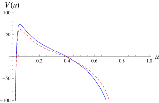
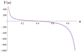
Figure 8: High temperature and low energy ($\bar{q}\,=\,0.3\bar{Q}^{3}$) longitudinal (left panel) and transversal (right panel) potentials of a flavour current (solid line) with $\theta_{0}\,=\,0.75$, compared to that of an ${\cal R}$ current (dashed line).

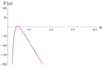
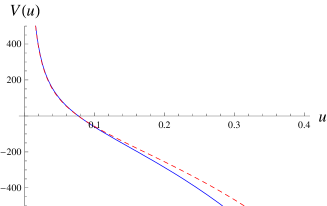
Figure 9: High temperature and high energy ($\bar{q}\,=\,1.6\bar{Q}^{3}$) longitudinal (left panel) and transversal (right panel) potentials of a flavour current (solid line) with $\theta_{0}\,=\,0.75$, compared to that of an ${\cal R}$ current (dashed line).

In the black hole embedding, an analysis of the eqs. (29) and (36) near the horizon $u=1$ leads to

$$a(x,u) = (1-u)^{\pm\,\frac{i}{2}\bar{w}}\left[\,\tilde{a}_{0}+\tilde{a}_{1}(1-u)+\tilde{a}_{2}(1-u)^{2}+\dots\,\,\right]\,,$$ (54)

$$A_{i}(x,u) = (1-u)^{\pm\,\frac{i}{2}\bar{w}}\left[\,\tilde{A}_{i,0}+\tilde{A}_{i,1}(1-u)+\tilde{A}_{i,2}(1-u)^{2}+\dots\,\,\right]\,\,.$$ (55)

So it is possible to impose an ingoing wave condition at the horizon, corresponding to choosing the exponent $-i\bar{w}/2$.

IV.2.1 Longitudinal contribution

Using the high energy approximation for the longitudinal potential near the boundary given in eq. (35) we have

$$\partial_{u}^{2}\psi\,+\,\left(\frac{1}{4u^{2}}\,+\,\bar{q}^{2}u\right)\psi\,=\,-\frac{m^{2}}{2}{\bar{q}}^{2}u^{2}\psi\,.$$ (56)

In the black hole phase the parameter $m$ satisfies the condition $m<1.31\,$. Then, near the boundary $m^{2}u$ is very small and the term on the rhs of eq. (56) can be neglected. Then we obtain the solution

$$\psi(x,u)\,=\,\bar{q}^{2}\left[A^{(0)}_{t}+\frac{\bar{w}}{\bar{q}}A^{(0)}_{3}\right]u^{1/2}\left[{\cal C}_{1}J_{0}(\frac{2}{3}\bar{q}u^{3/2})\,+\,{\cal C}_{2}Y_{0}(\frac{2}{3}\bar{q}u^{3/2})\right]\,,$$ (57)

where $J_{0}(z)$ and $Y_{0}(z)$ are Bessel functions, and ${\cal C}_{1}$, ${\cal C}_{2}$ are complex constants. Analysing the behaviour of this solution for large arguments of the Bessel functions we see that a progressive wave going from the boundary to the horizon can be obtained for ${\cal C}_{1}\,=\,-i\,{\cal C}_{2}$. So, we impose this condition and assume that the solution will remain an ingoing wave at the horizon.

In the limit $u\to 0$, relevant for the calculation of the retarded Green’s function, we can expand the Bessel functions finding

$$\psi(x,u) \,=\, \bar{q}^{2}\left[A^{(0)}_{t}+\frac{\bar{w}}{\bar{q}}A^{(0)}_{3}\right]u^{1/2}{\cal C}_{2}\Big{\{}-i\,+\,\frac{2}{\pi}\left[\ln(\frac{\bar{q}}{3}u^{3/2})+\gamma\right]$$ (58)

$$\,+\, {\cal O}(\bar{q}^{2}u^{3})\,+\,{\cal O}(\bar{q}^{2}u^{3})\ln(\frac{\bar{q}}{3}u^{3/2})\Big{\}}\,.$$

In the limit $u\to 0$, the perturbative corrections arising from the mass term of eq. (56) will be of order $u^{4}$, and so can be neglected with respect to the terms in eq. (58). Therefore, the mass term does not contribute to the Green’s function and hence to the DIS structure functions at high energies. Comparing the expansion (58) with (49) we find that

$${\cal C}_{2}\,=\ \frac{\pi}{3}\quad\,;\quad a_{0}\,=\,-i\,\frac{\pi}{3}\,+\,\frac{2}{3}\left(\ln{\frac{\bar{q}}{3}}+\gamma\right)\,.$$ (59)

The imaginary part of this expression will contribute to the DIS structure function.

IV.2.2 Transversal contribution

In the transversal case at high energies, using (41) we have

$$\partial_{u}^{2}\Phi_{i}\,+\,\bar{q}^{2}u\Phi_{i}\,=\,-\frac{m^{2}}{2}\bar{q}^{2}u^{2}\Phi_{i}\,.$$ (60)

As in the longitudinal case, we can neglect the mass term finding

$$\Phi_{i}(x,u)\,=\,A_{i}^{(0)}u^{1/2}\,\left[{\cal D}_{1}J_{1/3}(\frac{2}{3}\bar{q}u^{3/2})\,+\,{\cal D}_{2}Y_{1/3}(\frac{2}{3}\bar{q}u^{3/2})\right]\,,$$ (61)

The ingoing condition leads to ${\cal D}_{1}\,=\,-i{\cal D}_{2}$. In the limit $u\to 0$ we expand the Bessel functions as

$$\Phi_{i}(x,u)=A_{i}^{(0)}\,{\cal D}_{2}\left\{-\frac{\Gamma(\frac{1}{3})}{\pi}\left(\frac{\bar{q}}{3}\right)^{-\frac{1}{3}}+\frac{\sqrt{3}}{\Gamma(\frac{1}{3})}\left[-\sqrt{3}i+1\right]\left(\frac{\bar{q}}{3}\right)^{\frac{1}{3}}u+{\cal O}(\bar{q}^{2}u^{3})\right\}\,.$$ (62)

The perturbative correction to the function $\Phi_{i}$ coming from the mass term is real and of order $m^{2}u$. So it can be neglected in the high energy limit. Now, comparing the expansion (62) with (50) we find

$${\cal D}_{2}=-\frac{\pi}{\Gamma(1/3)}\left(\frac{\bar{q}}{3}\right)^{1/3}\,\,,\,\,c_{1}=-\frac{\sqrt{3}\pi}{\Gamma^{2}(1/3)}\left(\frac{\bar{q}}{3{\bar{Q}}^{3}}\right)^{2/3}+i\frac{3\pi}{\Gamma^{2}(1/3)}\left(\frac{\bar{q}}{3{\bar{Q}}^{3}}\right)^{2/3}\,,\,d_{1}=0\,.$$ (63)

IV.2.3 DIS structure functions

Using the results for the longitudinal and transversal potentials and the dictionary (47),(48) we obtain

$${R}_{1}\,=\,\frac{3}{2}\,\frac{\pi}{\Gamma^{2}(1/3)}\,N_{f}N_{c}T^{2}\left(\frac{\bar{q}}{3}\right)^{2/3}\,\left[-\frac{1}{\sqrt{3}}\,+\,i\right]\quad,\quad{R}_{2}\,=\,\frac{Q^{2}}{q^{2}}{R}_{1}\,.$$ (64)

Note that the imaginary part of $a_{0}$ was neglected with respect to the imaginary part of $c_{1}$. Then, the quark contributions to the plasma structure functions in the high energy limit are

$$F_{1}(x,Q^{2}) \,=\, \frac{1}{2\pi}{\rm Im}\,{R}_{1}\,\approx\,\frac{3}{4\Gamma^{2}(1/3)}\,N_{f}N_{c}T^{2}\left(\frac{Q^{2}}{12\pi T^{2}x}\right)^{2/3}$$

$$F_{2} \,=\, -\frac{n\cdot q}{2\pi T}\,{\rm Im}\,{R}_{2}\,\approx\,2xF_{1}\,,$$ (65)

where $x$ is the Bjorken variable that in the plasma rest frame takes the form $x=Q^{2}/2wT\,$.

These structure functions have the same dependence in the kinematic variables as the ${\cal R}$ current case discussed in section II. However the $N_{c}N_{f}$ factor contrasts with the $N^{2}_{c}$ factor of the ${\cal R}$ current. Explicitly, the plasma structure functions at high temperatures arising from the flavour current and ${\cal R}$ current are related by

$$\frac{F_{1,2}\,[{\rm flavour}]}{F_{1,2}\,[{\cal R}]}\,\approx\,4\,\frac{N_{f}}{N_{c}}\,.$$ (66)

This result can be interpreted in the following way. The ${\cal R}$ current interacts with fields in the adjoint representation of the $SU(N_{c})$ gauge group, that carry a number of degrees of freedom proportional to $N^{2}_{c}$. These fields describe gluons and their superpartners that are probed by the DIS of an ${\cal R}$ current. When we add the D7 probe branes, we include fields in the fundamental representation, that carry a number of degrees of freedom proportional to $N_{c}N_{f}$. These fields describe the quarks and their superpartners and are probed by the DIS of a flavour current. Note that the ratio $N_{f}/N_{c}$ was already found in Mateos:2007yp comparing the electric conductivities associated with a flavour current and an $\cal R$ current.

Note that our results for the structure functions $F_{1,2}$ at high energies hold for any value of the mass parameter $m$ lower than $1.31$, which corresponds to temperatures higher than $T_{c}=0.766M$. When the temperature decreases to $T=T_{c}$, the D7 brane embedding experiments a first order transition that takes it from a black hole to a Minkowski phase. As a consequence, the imaginary part of the gauge fields arising from the ingoing wave condition disappears leading to the vanishing of the quark contribution to the plasma structure functions, as we discussed in part A of this section.

V Conclusions

We studied the DIS off a ${\cal N}=2\,\,$ super Yang Mills plasma with flavour degrees of freedom using the holographic D3-D7 brane model at finite temperature. At high temperatures we found that the flavour current probes the partonic structure associated with the quark degrees of freedom in the same way as the ${\cal R}$ current probes the partonic structure associated with the gluonic degrees of freedom. At low temperatures the flavour current is not absorbed by the quark constituents of the plasma. As discussed above, this is a consequence of the abrupt change on the gauge fields behaviour far from the boundary due to the phase transition suffered by the D7 brane embedding.

Our results contrast with the gluonic sector, probed by an ${\cal R}$ current, that shows a partonic structure, associated with gluons, at any temperature. This might be related to the fact that in this model there is an effective infrared mass scale for the quark sector, but not for the gluon sector.

As we explained in this article, the non partonic absorption of the flavour current at low temperatures is a consequence of the absence of an imaginary part in the retarded Green’s function. It is important to remark that a real Green’s function may have poles and then give rise to imaginary contributions in the form of delta peaks. This kind of contribution was analysed in ref. Myers:2007we for a time-like flavour current in the low temperature Minkowski embedding. In that reference the delta peaks of the spectral function where interpreted in terms of the meson spectra. Here we have worked with a space-like flavour current and we did not consider this kind of contribution, since we were only interested in the partonic structure of the plasma.

After the first version of this article, ref. Iancu:2009py proposed a different mechanism for the absorption of a flavour current at low temperatures, based on vector meson production. This process contributes to the ${\cal N}=2\,\,$ super Yang Mills plasma structure functions of the D3-D7 brane model.

We worked in the probe approximation of the D3-D7 brane model in which the backreaction of the D7 branes is not taken into account. A review of the D3-D7 brane model beyond the probe limit was done in Erdmenger:2007cm . A recent proposal to include backreaction in the D3-D7 quark-gluon plasma appeared in Bigazzi:2009bk . It might be interesting to investigate the effect of these backreaction corrections on the plasma structure functions and on its partonic behaviour.

Acknowledgments: This work was originated in discussions with Edmond Iancu and Al Mueller. We also thank them for reading the manuscript and making various interesting comments. The authors are partially supported by CAPES, CNPq and FAPERJ.

References

- (1) E. Shuryak, Prog. Part. Nucl. Phys. 53, 273 (2004) [arXiv:hep-ph/0312227].
- (2) J. M. Maldacena, Adv. Theor. Math. Phys. 2, 231 (1998) [Int. J. Theor. Phys. 38, 1113 (1999)]. [arXiv:hep-th/9711200].
- (3) S. S. Gubser, I. R. Klebanov and A. M. Polyakov, Phys. Lett. B 428, 105 (1998). [arXiv:hep-th/9802109].
- (4) E. Witten, Adv. Theor. Math. Phys. 2, 253 (1998). [arXiv:hep-th/9802150].
- (5) J. Polchinski and M. J. Strassler, Phys. Rev. Lett. 88, 031601 (2002) [arXiv:hep-th/0109174].
- (6) H. Boschi-Filho and N. R. F. Braga, Phys. Lett. B 560, 232 (2003) [arXiv:hep-th/0207071].
- (7) H. Boschi-Filho and N. R. F. Braga, Eur. Phys. J. C 32, 529 (2004) [arXiv:hep-th/0209080].
- (8) H. Boschi-Filho and N. R. F. Braga, JHEP 0305, 009 (2003) [arXiv:hep-th/0212207].
- (9) G. F. de Teramond and S. J. Brodsky, Phys. Rev. Lett. 94, 201601 (2005) [arXiv:hep-th/0501022].
- (10) J. Erlich, E. Katz, D. T. Son and M. A. Stephanov, Phys. Rev. Lett. 95 (2005) 261602 [arXiv:hep-ph/0501128].
- (11) L. Da Rold and A. Pomarol, Nucl. Phys. B 721 (2005) 79 [arXiv:hep-ph/0501218].
- (12) H. Boschi-Filho, N. R. F. Braga and H. L. Carrion, Phys. Rev. D 73, 047901 (2006) [arXiv:hep-th/0507063].
- (13) A. Karch and E. Katz, JHEP 0206, 043 (2002) [arXiv:hep-th/0205236].
- (14) M. Kruczenski, D. Mateos, R. C. Myers and D. J. Winters, JHEP 0307, 049 (2003) [arXiv:hep-th/0304032].
- (15) J. Erdmenger, N. Evans, I. Kirsch and E. Threlfall, Eur. Phys. J. A 35 (2008) 81 [arXiv:0711.4467 [hep-th]].
- (16) J. Polchinski and M. J. Strassler, JHEP 0305, 012 (2003) [arXiv:hep-th/0209211].
- (17) C. A. Ballon Bayona, H. Boschi-Filho and N. R. F. Braga, JHEP 0803, 064 (2008) [arXiv:0711.0221 [hep-th]].
- (18) Y. Hatta, E. Iancu and A. H. Mueller, JHEP 0801, 026 (2008) [arXiv:0710.2148 [hep-th]].
- (19) C. A. Ballon Bayona, H. Boschi-Filho and N. R. F. Braga, JHEP 0810, 088 (2008) [arXiv:0712.3530 [hep-th]].
- (20) L. Cornalba and M. S. Costa, Phys. Rev. D 78, 096010 (2008) [arXiv:0804.1562 [hep-ph]].
- (21) B. Pire, C. Roiesnel, L. Szymanowski and S. Wallon, Phys. Lett. B 670, 84 (2008) [arXiv:0805.4346 [hep-ph]].
- (22) J. L. Albacete, Y. V. Kovchegov and A. Taliotis, JHEP 0807, 074 (2008) [arXiv:0806.1484 [hep-th]].
- (23) J. H. Gao and B. W. Xiao, Phys. Rev. D 80 (2009) 015025 [arXiv:0904.2870 [hep-ph]].
- (24) Y. Hatta, T. Ueda and B. W. Xiao, JHEP 0908 (2009) 007 [arXiv:0905.2493 [hep-ph]].
- (25) C. A. Ballon Bayona, H. Boschi-Filho and N. R. F. Braga, JHEP 0809, 114 (2008) [arXiv:0807.1917 [hep-th]].
- (26) L. Cornalba, M. S. Costa and J. Penedones, arXiv:0911.0043 [hep-th].
- (27) S. Hong, S. Yoon and M. J. Strassler, JHEP 0404, 046 (2004) [arXiv:hep-th/0312071].
- (28) H. R. Grigoryan and A. V. Radyushkin, Phys. Lett. B 650, 421 (2007) [arXiv:hep-ph/0703069].
- (29) H. R. Grigoryan and A. V. Radyushkin, Phys. Rev. D 76, 095007 (2007) [arXiv:0706.1543 [hep-ph]].
- (30) S. J. Brodsky and G. F. de Teramond, Phys. Rev. D 77, 056007 (2008) [arXiv:0707.3859 [hep-ph]].
- (31) H. J. Kwee and R. F. Lebed, Phys. Rev. D 77, 115007 (2008) [arXiv:0712.1811 [hep-ph]].
- (32) D. Rodriguez-Gomez and J. Ward, JHEP 0809, 103 (2008) [arXiv:0803.3475 [hep-th]].
- (33) C. A. B. Bayona, H. Boschi-Filho, N. R. F. Braga and M. A. C. Torres, JHEP 1001, 052 (2010) [arXiv:0911.0023 [hep-th]].
- (34) Y. Hatta, E. Iancu and A. H. Mueller, JHEP 0805, 037 (2008) [arXiv:0803.2481 [hep-th]].
- (35) Y. Hatta and T. Matsuo, Phys. Lett. B 670, 150 (2008) [arXiv:0804.4733 [hep-th]].
- (36) Y. Hatta and T. Matsuo, Phys. Rev. Lett. 102, 062001 (2009) [arXiv:0807.0098 [hep-ph]].
- (37) A. Vega, I. Schmidt, T. Branz, T. Gutsche and V. E. Lyubovitskij, Phys. Rev. D 80, 055014 (2009) [arXiv:0906.1220 [hep-ph]].
- (38) E. Witten, Adv. Theor. Math. Phys. 2, 505 (1998) [arXiv:hep-th/9803131].
- (39) D. T. Son and A. O. Starinets, JHEP 0209, 042 (2002) [arXiv:hep-th/0205051].
- (40) P. K. Kovtun and A. O. Starinets, Phys. Rev. D 72, 086009 (2005) [arXiv:hep-th/0506184].
- (41) Y. Hatta, E. Iancu and A. H. Mueller, JHEP 0801, 063 (2008) [arXiv:0710.5297 [hep-th]].
- (42) J. Babington, J. Erdmenger, N. J. Evans, Z. Guralnik and I. Kirsch, Phys. Rev. D 69, 066007 (2004) [arXiv:hep-th/0306018].
- (43) D. Mateos, R. C. Myers and R. M. Thomson, Phys. Rev. Lett. 97, 091601 (2006) [arXiv:hep-th/0605046].
- (44) C. Hoyos-Badajoz, K. Landsteiner and S. Montero, JHEP 0704, 031 (2007) [arXiv:hep-th/0612169].
- (45) D. Mateos, R. C. Myers and R. M. Thomson, JHEP 0705, 067 (2007) [arXiv:hep-th/0701132].
- (46) R. C. Myers, A. O. Starinets and R. M. Thomson, JHEP 0711, 091 (2007) [arXiv:0706.0162 [hep-th]].
- (47) D. Mateos and L. Patino, JHEP 0711, 025 (2007) [arXiv:0709.2168 [hep-th]].
- (48) E. Iancu and A. H. Mueller, JHEP 1002, 023 (2010) [arXiv:0912.2238 [hep-th]].
- (49) F. Bigazzi, A. L. Cotrone, J. Mas, A. Paredes, A. V. Ramallo and J. Tarrio, JHEP 0911, 117 (2009) [arXiv:0909.2865 [hep-th]].