Spinning compact binary inspiral:
Independent variables and dynamically preserved spin configurations

Abstract

We establish the set of independent variables suitable to monitor the complicated evolution of the spinning compact binary during the inspiral. Our approach is valid up to the second post-Newtonian order, including leading order spin-orbit, spin-spin and mass quadrupol-mass monopole effects, for generic (noncircular, nonspherical) orbits. Then we analyze the conservative spin dynamics in terms of these variables. We prove that the only binary black hole configuration allowing for spin precessions with equal angular velocities about a common intantaneous axis roughly aligned to the normal of the osculating orbit, is the equal mass and parallel (aligned or antialigned) spin configuration. This analytic result puts limitations on what particular configurations can be selected in numerical investigations of compact binary evolutions, even in those including only the last orbits of the inspiral.

I Introduction

Compact objects are characterized by their size and gravitational radius being comparable. They appear either as the end state of the stellar evolution as neutron stars or black holes with a few solar masses (M_⊙) or emerge from cosmological evolution by continued accretion and a sequence of mergers MergerTree  as supermassive black holes of $3\times 10^{6}\div 3\times 10^{9}$ M_⊙, residing in the centers of galaxies. Not much evidence has been gathered for the existence of intermediate mass black holes (IMBH), although a detection of a variable X-ray source of over 500 M_⊙ in the galaxy ESO 243-49 has been recently reported and interpreted as IMBH IMBH Nature . It has been proposed that IMBHs ought to be searched for in globular clusters that can be fitted well by medium-concentration King models IMBH Where .

Compact objects are expected to frequently coexist in binary systems, formed either by evolution of a stellar binary, by capture events or accompanying the process of galaxy mergers. According to general relativity, compact binaries radiate away gravitational waves, a process leading eventually to their merger. Stellar mass binaries are among the most prominent sources for the Earth-based gravitational wave detectors LIGO and Virgo LIGO , while the gravitational waves produced during the (low mass) galactic black hole mergers will be sought for by the long-planned space mission LISA LISA .

The merging process can be split into three distinct phases. By definition the inspiral is the regime of orbital evolution, which can be described accurately in terms of a post-Newtonian (PN) expansion. Provided the orbits are not excessively eccentric, the same PN parameter characterizes both weak gravity and non-relativistic motion:

$$\varepsilon=\frac{Gm}{c^{2}r}\approx\left(\frac{v}{c}\right)^{2}~{}.$$ (1)

A manifestly convergent and finite procedure for calculating gravitational radiation to arbitrary orders in a PN expansion was proposed convergenceWW , based on solving a flat-spacetime wave equation (representing Einstein equations with a harmonic gauge condition) as a retarded integral over the past null cone of the chosen field point. A study of the Cauchy convergence for PN templates shows an oscillatory behavior: increasing the PN order will not necessarily result in a better template CauchyPN (2PN templates being closer to numerical results, than their 2.5 counterparts). The predictions of various PN approximants (adiabatic Taylor, Padé models, non-adiabatic effective-one-body models) show that their convergence to numerical results is comparable convergenceTPEOB . It is also known, that alternative template families based on the shifted Chebyshev polynomials could exhibit faster Cauchy convergence, than PN templates CauchyChebyshev . Comparisons with full general relativistic numerical runs confirmed that a third PN order approach can be considered accurate for all practical purposes. The inspiral is followed by the plunge, where a full general relativistic treatment is necessary, and can be handled only numerically; and the ringdown, a process during which all physical characteristics of the newly formed compact object are radiated away, except mass, spin and possibly electric charge.

In this paper we investigate the conservative dynamics during the inspiral of a spinning compact binary system. We include spin-orbit (SO), spin-spin (SS) and mass quadrupole - mass monopole (QM) couplings, each to leading order. The precession due to these interactions was first discussed in BOC -BOC2 . With the spins and mass quadrupole moments included, the number of variables in the configuration space increases considerably, therefore we propose to find a minimal and conveniently chosen set of independent variables.

We note discussions of various aspects of the dynamics and gravitational radiation related to the SO coupling in KWW -Kidder , SS coupling in Kidder -spinspin2 , and QM coupling in Poisson -QM . PN corrections to the SO coupling were presented in PNSO and the Hamiltonian approach including spins has been also worked out Ham . Most recently, the back-reaction on the dynamics due to asymmetric gravitational wave emission in the spinning case, possibly leading to strong recoil effects, has been widely investigated, both analytically Kidder , recoilSpinningAnalytical and numerically for particular spin configurations recoilSpinningNumerical . Empirical formulae giving the ”final spin” have been advanced in Refs. finalspin and some of them compared in Barausse . Zoom-whirl orbits (generic for particles orbiting Kerr black holes zwKerr ) were also found in the framework of the PN formalism zwPN . A larger spin increases the likeliness of apparition of such orbits zwNumeric . Gravitational wave emission is hold responsible for the occurrence of the spin-flip phenomenon LeahyWilliams -Xspinflip in X-shaped radio galaxies LeahyWilliams , Xshape . Recently it has been shown, that for a typical merger of mass ratio at about $0.1$ the combined effect of SO precession and gravitational radiation will result in the spin-flip occurring during the inspiral SpinFlip .

In Sec. II we introduce the set of dynamical and configurational variables characterizing the compact spinning binary. Both the configurational and a subset of the dynamical variables depend on the choice of the reference system. We use a number of four such systems, to be defined in subsection II.2, only one of them inertial, the rest of three being rather adapted to the binary configuration. In subsection II.3 we derive two relations among the time derivatives of the introduced angular variables. As a result the time evolution of the configurational variables is determined by the evolution of one single configurational angle $\alpha$ and the true anomaly $\chi_{p}$. At the end of this section we express the position and velocity vectors in the chosen reference systems. As a by-product we recover the true anomaly parametrization of the radial evolution, valid for the chosen perturbed Keplerian setup.

Sec. III introduces the angles characterizing the angular momenta (total and orbital angular momenta and spins). The number of independent variables characterizing them is shown to be 6. We will chose them either as 5 angles and a scale, or equivalently as 3 angles and 3 scales.

In Sec. IV we analyze the conservative evolution of the spins, which is purely precessional, with the inclusion of the leading order spin-orbit, spin-spin and mass quadrupole - mass monopole couplings. We clarify the order (both PN and in the mass ratio) at which the various contributions occur. Then we investigate, whether there are spin configurations conserved by precessions, and we derive a no-go result.

The gravitational constant $G$ and speed of light $c$ are kept in all expressions. For any vector $\mathbf{V}$ we denote its Euclidean magnitude by $V$ and its direction by $\mathbf{\hat{V}}$.

II Kinematical and dynamical variables

II.1 Variables

We consider three distinct set of variables.

(a) The physical parameters of the binary: The two compact objects are characterized by masses $m_{i}$, spins $\mathbf{S}_{\mathbf{i}}$ ($i=1,2$), and mass quadrupole moments.

Equivalently to $m_{i}$ we can use the total mass $m\equiv m_{1}+m_{2}$ and the reduced mass $\mu\equiv m_{1}m_{2}/m$. We assume that $m_{1}\geq m_{2}$. We also introduce the mass ratio $\nu\equiv m_{2}/m_{1}\leq 1$ and the symmetric mass ratio $\eta\equiv\mu/m\in\left[0,0.25\right]$. The two mass ratios are related as

$$\eta=\frac{\nu}{\left(1+\nu\right)^{2}}~{},$$ (2)

and for small $\nu$ we have $\eta=\allowbreak\nu-2\nu^{2}+O\left(\nu^{3}\right)$. We also note the useful relations

$$m_{i}^{2}=m^{2}\eta\nu^{2i-3}~{}.$$ (3)

Equivalently to $\mathbf{S}_{\mathbf{i}}$ we can introduce their magnitude, polar and azimuthal angles. It is convenient to define dimensionless spin magnitudes $\chi_{i}\in\left[0,1\right]$ by

$$S_{i}\equiv\frac{G}{c}m_{i}^{2}\chi_{i}=\frac{G}{c}m^{2}\eta\nu^{2i-3}\chi_{i}~{}.$$ (4)

As for the spin angles, they depend on the chosen reference system. We will discuss various possibilities in detail in Section III.

We consider axisymmetric compact objects. Therefore the mass quadrupole of the $i^{th}$ axially symmetric binary component is characterized by a single quantity $Q_{i}$, its quadrupole-moment scalar Poisson . Provided the quadrupole moment originates entirely in its rotation (what we shall assume), then the symmetry axis is $\mathbf{\hat{S}}_{i}$ and

$$Q_{i}=-\frac{G^{2}}{c^{4}}w\chi_{i}^{2}m_{i}^{3}~{},$$ (5)

with the parameter $w\in\left(4,~{}8\right)$ for neutron stars, depending on their equation of state, stiffer equations of state giving larger values of $w$ Larakkers Poisson 1997 , Poisson . For rotating black holes $w=1$ Thorne 1980 . The negative sign arises because the rotating compact object is centrifugally flattened, becoming an oblate spheroid.

(b) Dynamical variables: Up to 2PN accuracy the energy $E$ and the total angular momentum vector $\mathbf{J\equiv L}+\mathbf{S}_{\mathbf{1}}+\mathbf{S}_{\mathbf{2}}$ are conserved KWW . The orbital angular momentum $\mathbf{L}$ and the spins $\mathbf{S}_{\mathbf{i}}$ are not conserved separately, as the spins undergo a precessional motion. This will be discussed in detail in Section IV.

(c) Angular variables characterizing the orbit:

The instantaneous orbital plane is perpendicular by definition to the Newtonian orbital angular momentum $\mathbf{L_{N}}\equiv\mu\mathbf{r}\times\mathbf{v}$ and it evolves due to the spin precessions. We define (i) the inclination $\alpha$ of the orbital plane with respect to the plane perpendicular to $\mathbf{J}$ (thus $\alpha$ is the angle span by $\mathbf{\hat{L}}_{\mathbf{N}}$ and $\mathbf{\hat{J}}$); (ii) the angle $\phi_{n}$ between the intersection $\mathbf{\hat{l}}$ of these two planes and an (arbitrary) inertial $x$-axis $\mathbf{\hat{x}}$ taken in the plane perpendicular to $\mathbf{J}$, finally (iii) the angle $\psi_{p}$ measured from $\mathbf{\hat{l}}$ to the periastron (see Figs 1 and 2; the indices $p$ and $n$ stand for the periastron and node line, respectively).

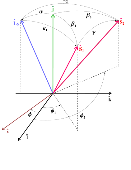
Figure 1: The polar and azimuthal angles of the total angular momentum $J\mathbf{\hat{J}}$, Newtonian orbital angular momentum $L_{N}\mathbf{\hat{L}}_{\mathbf{N}}$ and spins $S_{1,2}\mathbf{\hat{S}}_{\mathbf{1,2}}$. Azimuthal angles are shown in the non-inertial system $\mathcal{K}_{J}\equiv\left(\mathbf{\hat{l},\hat{k},\hat{J}}\right)$, polar angles both in $\mathcal{K}_{J}$ and respective to $\mathbf{\hat{L}}_{\mathbf{N}}$. The relative angle of the spins is $\gamma$. The non-inertial character of the system $\mathcal{K}_{J}$ is encoded in the evolution of the angle $\phi_{n}$, measuring the angular separation of an inertial axis $\mathbf{\hat{x}}$ from the axis $\mathbf{\hat{l}}$.

II.2 Reference systems

For a better bookkeeping we introduce the inertial system $\mathcal{K}_{i}$ with $\mathbf{\hat{x}}$ and $\mathbf{\hat{J}}$ standing as the $x$- and $z$-axes and three non-inertial systems $\mathcal{K}_{J}$, $\mathcal{K}_{L}$ and $\mathcal{K}_{A}$.

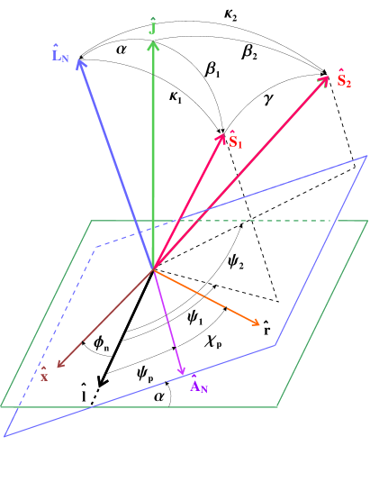
Figure 2: The relative angles of the total angular momentum $J\mathbf{\hat{J}}$, Newtonian orbital angular momentum $L_{N}\mathbf{\hat{L}}_{\mathbf{N}}$ and spins $S_{1,2}\mathbf{\hat{S}}_{\mathbf{1,2}}$ as in Fig 1. The intersection of the planes perpendicular to $\mathbf{\hat{L}}_{\mathbf{N}}$ and $\mathbf{\hat{J}}$, respectively is the node line $\mathbf{\hat{l}}$. The inertial axis $\mathbf{\hat{x}}$ is at angle $\phi_{n}$, measured from $\mathbf{\hat{l}}$ in the plane perpendicular to $\mathbf{\hat{J}}$. The azimuthal angles $\left(\psi_{1},\psi_{2},\psi_{p}\right)$ of the spins and Newtonian Laplace-Runge-Lenz vector $A_{N}\mathbf{\hat{A}}_{\mathbf{N}}$ (pointing towards the periastron) are also measured from $\mathbf{\hat{l}}$, however in the plane perpendicular to $\mathbf{\hat{L}}_{\mathbf{N}}$. The true anomaly $\chi_{p}$ is the angle between $\mathbf{\hat{A}}_{\mathbf{N}}$ and the position vector $r\mathbf{\hat{r}}$. Two of the basis vectors of the inertial reference system $\mathcal{K}_{i}\equiv\left(\mathbf{\hat{x},\hat{y},\hat{J}}\right)$ and of each of the three non-inertial reference systems $\mathcal{K}_{J}\equiv\left(\mathbf{\hat{l},\hat{k},\hat{J}}\right)$, $\mathcal{K}_{L}\equiv\left(\mathbf{\hat{l},\hat{m},\hat{L}}_{\mathbf{N}}\right)$, $\mathcal{K}_{A}\equiv\left(\mathbf{\hat{A}}_{\mathbf{N}}\mathbf{,\hat{Q}}_{\mathbf{N}}\mathbf{,\hat{L}}_{\mathbf{N}}\right)$ are shown.

In the system $\mathcal{K}_{J}$ the $z$-axis is fixed along $\mathbf{\hat{J}}$, while in $\mathcal{K}_{L}$ along $\mathbf{\hat{L}}_{\mathbf{N}}$. We choose $\mathbf{\hat{l}}=\mathbf{\hat{J}}\times\mathbf{\hat{L}}_{\mathbf{N}}/\sin\alpha$ as the $x$-axis of both systems. The system $\mathcal{K}_{J}$ is complete by $\mathbf{\hat{k}=\hat{J}}\times\mathbf{\hat{l}}$ and $\mathcal{K}_{L}$ by $\mathbf{\hat{m}=\hat{L}}_{\mathbf{N}}\times\mathbf{\hat{l}}$.

The system $\mathcal{K}_{A}$ also has $\mathbf{\hat{L}}_{\mathbf{N}}$ as the $z$-axis, however its $x$-axis is defined by the Laplace-Runge-Lenz vector

$$\mathbf{A}_{\mathbf{N}}\equiv\mathbf{v}\times\mathbf{L}_{\mathbf{N}}-\frac{Gm\mu}{r}\mathbf{r}\ ,$$ (6)

which satisfies the constraints

$$A_{N}^{2}=\frac{2E_{N}L_{N}^{2}}{\mu}+(Gm\mu)^{2}\ ,$$ (7)

and $\mathbf{L}_{\mathbf{N}}\mathbf{\cdot A}_{\mathbf{N}}=0$. Here $\mathbf{r}$ and $\mathbf{v}$ are the position vector and velocity of the reduced mass particle orbiting $m$. The $y$-axis is defined by $\mathbf{Q}_{\mathbf{N}}\equiv\mathbf{L}_{\mathbf{N}}\times\mathbf{A}_{\mathbf{N}}$. The orthonormal basis of $\mathcal{K}_{A}$ is therefore $(\mathbf{\hat{A}}_{\mathbf{N}},\ \mathbf{\hat{Q}}_{\mathbf{N}},~{}\mathbf{\hat{L}}_{\mathbf{N}})$.

The three angles $\left(\phi_{n},\alpha,\psi_{p}\right)$ will be referred to occasionally as Euler angles, as three consecutive rotations with $-\phi_{n},~{}\alpha$ and $\psi_{p}$ about the axes $z,~{}x$ and again $z$ transform as $\mathcal{K}_{i}\rightarrow$ $\mathcal{K}_{J}\rightarrow$ $\mathcal{K}_{L}\rightarrow$ $\mathcal{K}_{A}$. The sequence of these rotations is encompassed in the transformation matrix

$$\mathcal{R}\left(-\phi_{n},\alpha,\psi_{p}\right) = \mathcal{R}_{z}\left(\psi_{p}\right)\mathcal{R}_{x}\left(\alpha\right)\mathcal{R}_{z}\left(-\phi_{n}\right)$$ (11)

$$= \left(\begin{array}[]{ccc}\cos\psi_{p}\cos\phi_{n}+\sin\psi_{p}\cos\alpha\sin\phi_{n}&-\cos\psi_{p}\sin\phi_{n}+\sin\psi_{p}\cos\alpha\cos\phi_{n}&\sin\psi_{p}\sin\alpha\\ -\sin\psi_{p}\cos\phi_{n}+\cos\psi_{p}\cos\alpha\sin\phi_{n}&\sin\psi_{p}\sin\phi_{n}+\cos\psi_{p}\cos\alpha\cos\phi_{n}&\cos\psi_{p}\sin\alpha\\ -\sin\alpha\sin\phi_{n}&-\sin\alpha\cos\phi_{n}&\cos\alpha\end{array}\right)~{},$$

where $\mathcal{R}$ with one argument denotes the corresponding rotation matrices acting on the coordinates.

II.3 Constraints on the Euler angle evolutions

The coordinates of the reduced mass particle in the inertial system $\mathcal{K}_{i}$ can be obtained by applying the transformation $\mathcal{R}\left(-\psi,-\alpha,\phi_{n}\right)$ to the coordinates of the vector $\mathbf{r}=r\left(1,0,0\right)$. Here $\psi$ $=\psi_{p}+\chi_{p}$ is the angle span by $\mathbf{\hat{l}}$ and $\mathbf{\hat{r}}$, with $\chi_{p}$ defined as the true anomaly, the angle span by $\mathbf{\hat{A}}_{\mathbf{N}}$ and $\mathbf{\hat{r}}$. We obtain

$$\left(\begin{array}[]{c}x\\ y\\ z\end{array}\right)=r\left(\begin{array}[]{c}\cos\phi_{n}\cos\psi+\sin\phi_{n}\cos\alpha\sin\psi\\ -\sin\phi_{n}\cos\psi+\cos\phi_{n}\cos\alpha\sin\psi\\ \sin\alpha\sin\psi\end{array}\right)~{}.$$ (12)

A tedious, but straightforward computation carried on in the system $K_{i}$ gives

$$\frac{\mathbf{L_{N}}}{{\mu r}^{2}} = \dot{\phi}_{n}\left(\begin{array}[]{c}\sin\alpha\sin\psi\left[\cos\phi_{n}\cos\psi+\sin\phi_{n}\cos\alpha\sin\psi\right]\\ \sin\alpha\sin\psi\left[-\sin\phi_{n}\cos\psi+\cos\phi_{n}\cos\alpha\sin\psi\right]\\ \sin^{2}\alpha\sin^{2}\psi-1\end{array}\right)$$ (24)

$$+\dot{\alpha}\sin\psi\left(\begin{array}[]{c}-\sin\phi_{n}\cos\alpha\cos\psi+\cos\phi_{n}\sin\psi\\ -\cos\phi_{n}\cos\alpha\cos\psi-\sin\phi_{n}\sin\psi\\ -\sin\alpha\cos\psi\end{array}\right)$$

$$+\dot{\psi}\left(\begin{array}[]{c}-\sin\phi_{n}\sin\alpha\\ -\cos\phi_{n}\sin\alpha\\ \cos\alpha\end{array}\right)~{}.$$

From here we readily obtain

$$\frac{L_{N}^{2}}{{\mu}^{2}{r}^{4}}=\left(\dot{\psi}-\dot{\phi}_{n}\cos\alpha\right)^{2}+\left(\dot{\phi}_{n}\sin\alpha\cos\psi+\dot{\alpha}\sin\psi\right)^{2}~{}.$$ (25)

Also, dividing the third component (which by definition is $\left(\mathbf{L_{N}}\right)_{z}=L_{N}\cos\alpha$) by $\cos\alpha$ we get

$$\frac{L_{N}}{{\mu r}^{2}}=\dot{\psi}-\dot{\phi}_{n}\cos\alpha-\left(\dot{\phi}_{n}\sin\alpha\cos\psi+\dot{\alpha}\sin\psi\right)\tan\alpha\cos\psi~{}.$$ (26)

In the Newtonian approximation the Euler angles being constant, we recover $L_{N}=\mu r^{2}\dot{\chi}_{p}$ and $\left(\mathbf{L_{N}}\right)_{z}=\mu r^{2}\dot{\chi}_{p}\cos\alpha$.

By squaring Eq. (26) and subtracting from Eq. (25) we obtain the identity:

$$0 = \left[\left(1-\tan^{2}\alpha\cos^{2}\psi\right)\left(\dot{\phi}_{n}\sin\alpha\cos\psi+\dot{\alpha}\sin\psi\right)+2\tan\alpha\cos\psi\left(\dot{\psi}-\dot{\phi}_{n}\cos\alpha\right)\right]$$ (27)

$$\times\left(\dot{\phi}_{n}\sin\alpha\cos\psi+\dot{\alpha}\sin\psi\right)~{}.$$

The first factor cannot vanish, as to Newtonian order it gives $2\tan\alpha\cos\psi L_{N}/\mu r^{2}\neq 0$, therefore the vanishing of the second factor (by reintroducing $\psi=\psi_{p}+\chi_{p}$) gives:

$$\dot{\phi}_{n}=-\dot{\alpha}\frac{\tan\left(\psi_{p}+\chi_{p}\right)}{\sin\alpha}~{}.$$ (28)

Reinserting this in either of the Eqs. (25) or (26) gives

$$\dot{\psi}_{p}+\dot{\chi}_{p}=\frac{L_{N}}{{\mu r}^{2}}+\dot{\phi}_{n}\cos\alpha~{}.$$ (29)

We have just derived two relations among the time derivatives of the Euler angles and of the true anomaly, which restrict the number of independent angular variables introduced up to now to $\alpha$ and $\chi_{p}$.

II.4 The position and velocity vectors in the bases $\mathcal{K}_{A}$ and $\mathcal{K}_{L}$

Simple computation starting from the definitions of $\mathbf{A}_{\mathbf{N}}$ and $\mathbf{Q}_{\mathbf{N}}$ gives

$$\mathbf{A}_{\mathbf{N}} = \mu\left(\frac{2E_{N}}{\mu}+\frac{Gm}{r}\right)\mathbf{r-}\mu r\dot{r}\mathbf{v}\ ,$$

$$\mathbf{Q}_{\mathbf{N}} = Gm\mu^{2}\dot{r}\mathbf{r+}\left(L_{N}^{2}-Gm\mu^{2}r\right)\mathbf{v}\ .$$ (30)

From here the expressions of the position and velocity vectors in $\mathcal{K}_{A}$ emerge as

$$\mathbf{r} = \frac{L_{N}^{2}-Gm\mu^{2}r}{\mu A_{N}}\mathbf{\hat{A}}_{\mathbf{N}}+\frac{L_{N}}{A_{N}}r\dot{r}\mathbf{\hat{Q}}_{\mathbf{N}}\ ,$$ (31)

$$\mathbf{v} = -\frac{Gm\mu}{A_{N}}\dot{r}\mathbf{\hat{A}}_{\mathbf{N}}+\frac{L_{N}}{A_{N}}\left(\frac{2E_{N}}{\mu}+\frac{Gm}{r}\right)\mathbf{\hat{Q}}_{\mathbf{N}}\ .$$ (32)

In terms of the true anomaly $\chi_{p}$ (the azimuthal angle of $\mathbf{r}$ in the system $\mathcal{K}_{A}$), the position vector is given by

$$\mathbf{r}=r\left(\cos\chi_{p}\mathbf{\hat{A}}_{\mathbf{N}}+\sin\chi_{p}\mathbf{\hat{Q}}_{\mathbf{N}}\right)\mathbf{~{},}$$ (33)

which compared with Eq. (31) gives the true anomaly parametrization:

$$r = \frac{L_{N}^{2}}{\mu\left(Gm\mu+A_{N}\cos\chi_{p}\right)}~{},$$ (34)

$$\dot{r} = \frac{A_{N}}{L_{N}}\sin\chi_{p}~{}.$$ (35)

In terms of the true anomaly, the velocity is expressed as

$$\mathbf{v}=\frac{Gm\mu}{L_{N}}\left[-\sin\chi_{p}\mathbf{\hat{A}}_{\mathbf{N}}+\left(\cos\chi_{p}+\frac{A_{N}}{Gm\mu}\right)\mathbf{\hat{Q}}_{\mathbf{N}}\right]\ .$$ (36)

Its square gives $v^{2}$ in terms of the true anomaly:

$$v^{2}=\frac{\left(Gm\mu\right)^{2}+A_{N}^{2}+2Gm\mu A_{N}\cos\chi_{p}}{L_{N}^{2}}~{}.$$ (37)

(The same emerges from the definition of the Newtonian energy $E_{N}\equiv\mu v^{2}/2-Gm\mu/r$, by applying Eqs. (7) and (34).)

As the basis vectors of $\mathcal{K}_{A}$ are related to the basis vectors of $\mathcal{K}_{L}$ by a rotation with angle $\psi_{p}$:

$$\mathbf{\hat{A}}_{\mathbf{N}} = \cos\psi_{p}\mathbf{\hat{l}}+\sin\psi_{p}\mathbf{\hat{m}~{},}$$

$$\mathbf{\hat{Q}}_{\mathbf{N}} = -\sin\psi_{p}\mathbf{\hat{l}}+\cos\psi_{p}\mathbf{\hat{m}~{},}$$ (38)

it is straightforward to rewrite $\mathbf{r}$ and $\mathbf{v}$ in the basis $\mathcal{K}_{L}$ as

$$\mathbf{r} = r\left(\cos\psi\mathbf{\hat{l}}+\sin\psi\mathbf{\hat{m}}\right)\ ,$$ (39)

$$\mathbf{v} = \frac{1}{L_{N}}\left[-\left(Gm\mu\sin\psi+A_{N}\sin\psi_{p}\right)\mathbf{\hat{l}}+\left(Gm\mu\cos\psi+A_{N}\cos\psi_{p}\right)\mathbf{\hat{m}}\right]\ .$$ (40)

III Constraints on angular momentum variables

III.1 The 5 angular degrees of freedom

The polar and azimuthal angles of $\mathbf{\hat{L}}_{\mathbf{N}}$ and $\mathbf{\hat{S}_{i}}$ in $\mathcal{K}_{J}$ are ($\alpha,-\pi/2$) and ($\beta_{i},\phi_{i}$), respectively, such that

$$\mathbf{\hat{L}}_{\mathbf{N}} = -\sin\alpha\mathbf{\hat{k}}+\cos\alpha\mathbf{\hat{J}}~{},$$ (41)

$$\mathbf{\hat{S}_{i}} = \sin\beta_{i}\cos\phi_{i}\mathbf{\hat{l}}+\sin\beta_{i}\sin\phi_{i}\mathbf{\hat{k}}+\cos\beta_{i}\mathbf{\hat{J}}~{}.$$ (42)

Similarly, the polar and azimuthal angles of $\mathbf{\hat{J}}$ and $\mathbf{\hat{S}_{i}}$ in $\mathcal{K}_{L}$ are ($\alpha,\pi/2$) and ($\kappa_{i},\psi_{i}$), respectively, thus

$$\mathbf{\hat{J}} = \sin\alpha\mathbf{\hat{m}}+\cos\alpha\mathbf{\hat{L}}_{\mathbf{N}}~{},$$ (43)

$$\mathbf{\hat{S}_{i}} = \sin\kappa_{i}\cos\psi_{i}\mathbf{\hat{l}}+\sin\kappa_{i}\sin\psi_{i}\mathbf{\hat{m}+}\cos\kappa_{i}\mathbf{\hat{L}}_{\mathbf{N}}~{}.$$ (44)

By comparing the two forms of the $\mathbf{\hat{l}}$ component of the vectors $\mathbf{\hat{S}_{i}}$ we get

$$\sin\kappa_{i}\cos\psi_{i}=\sin\beta_{i}\cos\phi_{i}~{}.$$ (45)

By computing $\mathbf{\hat{S}_{i}\cdot\hat{L}}_{\mathbf{N}}$ in both systems we find

$$\cos\kappa_{i}\mathbf{=}\cos\alpha\cos\beta_{i}-\sin\alpha\sin\beta_{i}\sin\phi_{i}~{}.$$ (46)

As $\sin\phi_{i}=-\cos\left(\pi/2+\phi_{i}\right)$ and $\pi/2+\phi_{i}$ is the relative azimuthal angle of $\mathbf{\hat{L}}_{\mathbf{N}}$ and $\mathbf{\hat{S}_{i}}$, Eq. (46) is but the spherical cosine identity in the triangle defined by these three vectors on the unit sphere.

Similarly, from the two expressions $\mathbf{\hat{S}_{1}\cdot\hat{S}_{2}}\equiv\cos\gamma$ written in both reference systems we find the spherical cosine identities:

$$\cos\gamma = \cos\kappa_{1}\cos\kappa_{2}+\sin\kappa_{1}\sin\kappa_{2}\cos\Delta\psi~{},$$ (47)

$$\cos\gamma = \cos\beta_{1}\cos\beta_{2}+\sin\beta_{1}\sin\beta_{2}\cos\Delta\phi~{}.$$ (48)

where $\Delta\psi=\psi_{2}-\psi_{1}$ and $\Delta\phi=\phi_{2}-\phi_{1}$ are the differences in the azimuthal angles of the two spins in the two systems $\mathcal{K}_{L}$ and $\mathcal{K}_{J}$, respectively.

Other spherical triangle identities arise by computing $\mathbf{\hat{S}_{i}\cdot\hat{J}}$ in both systems:

$$\cos\beta_{i}=\cos\alpha\cos\kappa_{i}+\sin\alpha\sin\kappa_{i}\sin\psi_{i}~{}.$$ (49)

Then Eqs. (45) and (49) give $\beta_{i},\phi_{i}$ as function of $\kappa_{i},\psi_{i}$ and $\alpha$. Inserting these in Eqs. (47) and (48) and eliminating $\gamma$ could in principle give $\alpha$ as function of $\kappa_{i},\psi_{i}$ alone. We get:

$$\sin\beta_{1}\sin\phi_{1}\sin\beta_{2}\sin\phi_{2}=\left(\sin\alpha\cos\kappa_{1}-\cos\alpha\sin\kappa_{1}\sin\psi_{1}\right)\left(\sin\alpha\cos\kappa_{2}-\cos\alpha\sin\kappa_{2}\sin\psi_{2}\right)~{}.$$ (50)

As the orientation of the spins are independent, we obtain

$$\sin\beta_{i}\sin\phi_{i}=\sin\alpha\cos\kappa_{i}-\cos\alpha\sin\kappa_{i}\sin\psi_{i}~{},$$ (51)

however the direct computation of the left hand side by employing Eqs. (45) and (49) results in the right hand side, leading to an identity rather than an expression of $\alpha$ as function of $\kappa_{i},\psi_{i}$. Therefore Eq. (48) can be considered as a consequence of the other equations. Similarly one can show that Eqs. (46) are consequences of the other equations.

We conclude that there are 5 independent constraint equations for the 10 angles ($\alpha,\beta_{i},\phi_{i},\kappa_{i},\psi_{i},\gamma$), namely Eqs. (45), (49) and (47), and we can take ($\alpha,\kappa_{i},\psi_{i}$) as the independent angles. The network of all angles in the systems $K_{J}$ and $K_{L}$ is represented on Figs 1 and 2, respectively.

III.2 Orbital angular momentum

The total orbital angular momentum $\mathbf{L}$ contains pure general relativistic (PN, 2PN) and spin-orbit (SO) contributions Kidder :

$$\mathbf{L}=\mathbf{L_{N}}+\mathbf{L_{PN}}+\mathbf{L_{SO}+L_{2PN}}\ .$$ (52)

There are no spin-spin or quadrupole-monopole contributions to the orbital angular momentum quadrup . Here the $\mathbf{L_{PN}}$ and $\mathbf{L_{2PN}}$ contributions are aligned to $\mathbf{L_{N}}$ (cf. Eq. (2.9) of Ref. Kidder ):

$$\mathbf{L}_{\mathbf{PN}} = \epsilon_{PN}\mathbf{L}_{\mathbf{N}}\ ,$$

$$\epsilon_{PN} = \frac{1-3\eta}{2}\left(\frac{v}{c}\right)^{2}+\left(3+\eta\right)\frac{Gm}{c^{2}r}~{},$$ (53)

and

$$\mathbf{L}_{2\mathbf{PN}} = \epsilon_{2PN}\mathbf{L}_{\mathbf{N}}\ ,$$

$$\epsilon_{2PN} = \frac{3}{8}\left(1-7\eta+13\eta^{2}\right)\left(\frac{v}{c}\right)^{4}-\frac{1}{2}\eta\left(2+5\eta\right)\frac{Gm}{c^{2}r}\left(\frac{\dot{r}}{c}\right)^{2}$$ (54)

$$+\frac{1}{2}\left(7-10\eta-9\eta^{2}\right)\frac{Gm}{c^{2}r}\left(\frac{v}{c}\right)^{2}+\frac{1}{4}\left(14-41\eta+4\eta^{2}\right)\left(\frac{Gm}{c^{2}r}\right)^{2}~{}.$$

The SO contribution (Eq. (2.9.c) of Ref. Kidder ) can be rewritten as

$$\mathbf{L_{SO}} = \sum_{i=1}^{2}S_{i}\left[\epsilon_{\mathbf{i}}^{\mathbf{r}}\left(\mathbf{\hat{r}}\cdot\mathbf{\hat{S}_{i}}\right)\mathbf{\hat{r}}+\epsilon_{\mathbf{i}}^{\mathbf{v}}\left(\mathbf{\hat{v}}\cdot\mathbf{\hat{S}_{i}}\right)\mathbf{\hat{v}-}\left(\epsilon_{\mathbf{i}}^{\mathbf{r}}+\epsilon_{\mathbf{i}}^{\mathbf{v}}\right)\mathbf{\hat{S}_{i}}\right]~{},$$

$$\epsilon_{\mathbf{i}}^{\mathbf{r}} = {\frac{Gm}{c^{2}r}\eta}\left(2+\nu^{3-2i}\right)$$

$$\epsilon_{\mathbf{i}}^{\mathbf{v}} = -{\frac{v^{2}}{2c^{2}}\eta}\nu^{3-2i}~{}.$$ (55)

Note that

$$\epsilon_{PN} = \mathcal{O}\left(\varepsilon\right)\mathcal{O}\left(1,\eta\right)~{},$$

$$\epsilon_{2PN} = \mathcal{O}\left(\varepsilon^{2}\right)\mathcal{O}\left(1,\eta,\eta^{2}\right)~{},$$ (56)

and

$$\epsilon_{\mathbf{i}}^{\mathbf{r}} = \mathcal{O}\left(\varepsilon\right)\mathcal{O}\left(\eta\right)\mathcal{O}\left(1,\nu^{3-2i}\right)~{},$$

$$\epsilon_{\mathbf{i}}^{\mathbf{v}} = \mathcal{O}\left(\varepsilon\right)\mathcal{O}\left(\eta\right)\mathcal{O}\left(\nu^{3-2i}\right)~{}.$$ (57)

In order to evaluate the PN order of the $\mathbf{L_{SO}}$ contribution in $\mathbf{J}$, we evaluate on circular orbits

$$\frac{S_{i}}{L_{N}} = \frac{\left(G/c\right)m^{2}\eta\nu^{2i-3}\chi_{i}}{\mu rv}=\left(\frac{Gm}{c^{2}r}\right)\frac{c}{v}\nu^{2i-3}\chi_{i}$$ (58)

$$= \mathcal{O}\left(\varepsilon^{1/2}\right)\mathcal{O}\left(\nu^{2i-3}\right)\chi_{i}~{},$$

which continue to approximately hold for eccentric orbits. This reasoning shows that the SO contribution is of 1.5 PN order and also indicates how to pick up the dominant terms when the mass ratio is small or when one would like to employ a less accurate, but simpler description, dropping higher order terms.

The total angular momentum is then

$$J\mathbf{\hat{J}}=\left(1+\epsilon_{PN}+\epsilon_{2PN}\right)L_{N}\mathbf{\hat{L}}_{\mathbf{N}}+\sum_{i=1}^{2}S_{i}\left[\epsilon_{\mathbf{i}}^{\mathbf{r}}\left(\mathbf{\hat{r}}\cdot\mathbf{\hat{S}_{i}}\right)\mathbf{\hat{r}}+\epsilon_{\mathbf{i}}^{\mathbf{v}}\left(\mathbf{\hat{v}}\cdot\mathbf{\hat{S}_{i}}\right)\mathbf{\hat{v}+}\left(1\mathbf{-}\epsilon_{\mathbf{i}}^{\mathbf{r}}-\epsilon_{\mathbf{i}}^{\mathbf{v}}\right)\mathbf{\hat{S}_{i}}\right]\ .$$ (59)

III.3 One scaling degree of freedom

In this subsection we will employ the projections of the Eq. (59) in order to derive relations between the angles and magnitudes of the angular momenta involved. In the $\mathcal{K}_{L}$ system the projections along the axes $\mathbf{\hat{l}}$, $\mathbf{\hat{m}}$ and $\mathbf{\hat{L}}_{\mathbf{N}}$ give, respectively:

$$0 = \sum_{i=1}^{2}S_{i}\sin\kappa_{i}\left\{\left(1\mathbf{-}\epsilon_{\mathbf{i}}^{\mathbf{r}}-\epsilon_{\mathbf{i}}^{\mathbf{v}}\right)\cos\psi_{i}+\epsilon_{\mathbf{i}}^{\mathbf{r}}\cos\left(\psi-\psi_{i}\right)\cos\psi+\epsilon_{\mathbf{i}}^{\mathbf{v}}\mathcal{S}\left[Gm\mu\sin\left(\psi-\psi_{i}\right)+A_{N}\sin\left(\psi_{p}-\psi_{i}\right)\right]\right\}\ ,$$ (60)

$$J\sin\alpha = \sum_{i=1}^{2}S_{i}\sin\kappa_{i}\left\{\left(1\mathbf{-}\epsilon_{\mathbf{i}}^{\mathbf{r}}-\epsilon_{\mathbf{i}}^{\mathbf{v}}\right)\sin\psi_{i}+\epsilon_{\mathbf{i}}^{\mathbf{r}}\cos\left(\psi-\psi_{i}\right)\sin\psi-\epsilon_{\mathbf{i}}^{\mathbf{v}}\mathcal{C}\left[Gm\mu\sin\left(\psi-\psi_{i}\right)+A_{N}\sin\left(\psi_{p}-\psi_{i}\right)\right]\right\}\ ,$$ (61)

$$J\cos\alpha = L_{N}\left(1+\epsilon_{PN}+\epsilon_{2PN}\right)+\sum_{i=1}^{2}S_{i}\left(1\mathbf{-}\epsilon_{\mathbf{i}}^{\mathbf{r}}-\epsilon_{\mathbf{i}}^{\mathbf{v}}\right)\cos\kappa_{i}\ ,$$ (62)

where

$$\mathcal{S}\left(\chi_{p},\psi_{p}\right) = \frac{Gm\mu\sin\left(\psi_{p}+\chi_{p}\right)+A_{N}\sin\psi_{p}}{\left(Gm\mu\right)^{2}+A_{N}^{2}+2Gm\mu A_{N}\cos\chi_{p}}~{},$$

$$\mathcal{C}\left(\chi_{p},\psi_{p}\right) = \frac{Gm\mu\cos\left(\psi_{p}+\chi_{p}\right)+A_{N}\cos\psi_{p}}{\left(Gm\mu\right)^{2}+A_{N}^{2}+2Gm\mu A_{N}\cos\chi_{p}}~{}.$$ (63)

In the derivation of Eqs. (60)-(62) we have employed Eqs. (39), (40), (43), (44) from where we also obtained

$$\mathbf{\hat{r}}\cdot\mathbf{\hat{S}_{i}} = \sin\kappa_{i}\cos\left(\psi-\psi_{i}\right)~{},$$ (64)

$$\mathbf{\hat{v}}\cdot\mathbf{\hat{S}_{i}} \mathbf{=} \frac{\sin\kappa_{i}}{L_{N}v}\left[-Gm\mu\sin\left(\psi-\psi_{i}\right)+A_{N}\sin\left(\psi_{i}-\psi_{p}\right)\right]~{},$$ (65)

with $v$ given by Eq. (37).

We thus have introduced the 14 quantities ($J,L,\chi_{i},\alpha,\beta_{i},\phi_{i},\kappa_{i},\psi_{i},\gamma$) describing the angular momenta, which are constrained by 8 independent  relations. This leaves us with 6 independent variables. 5 of these can be thought as the angles defining the directions of the spins and orbital angular momentum in the $K_{L}$ system ($\alpha,\kappa_{i},\psi_{i}$), a sixth one being a linear scale, most conveniently chosen as $J$.

Note that in Eqs. (60)-(62) the coefficients $\epsilon_{PN}$, $\epsilon_{2PN}$, $\epsilon_{\mathbf{i}}^{\mathbf{r}}$, $\epsilon_{\mathbf{i}}^{\mathbf{v}}$ depend only on the masses and $\chi_{p}$. Therefore all dependences on $\psi_{i}$ are explicit. In principle Eqs. (60)-(61) can be used to express $\psi_{i}$ as function of $\kappa_{i}$, $\alpha$, $\psi_{p}$, the masses and the spins $\chi_{i}$. In practice however this may be cumbersome. The easiest way to do it is to rewrite both the $\sin\psi_{i}$ and $\cos\psi_{i}$ in terms of the variables $x_{i}=\tan\psi_{i}/2$. Then Eqs. (60)-(61) become second rank coupled polynomial equations, possibly leading to two distinct values of $\psi_{i}$ for each $\chi_{i}$.

Finally, Eq. (62) can be employed to eliminate $L_{N}$ in the detriment of the angular variables, spins and $J$, by a series expansion in $\varepsilon$ to 2PN order accuracy as

$$L_{N} = J\left(1-\epsilon_{PN}+\epsilon_{PN}^{2}-\epsilon_{2PN}\right)\cos\alpha-\sum_{i=1}^{2}S_{i}\left(1-\epsilon_{PN}-\epsilon_{\mathbf{i}}^{\mathbf{r}}-\epsilon_{\mathbf{i}}^{\mathbf{v}}+\epsilon_{PN}\epsilon_{\mathbf{i}}^{\mathbf{r}}+\epsilon_{PN}\epsilon_{\mathbf{i}}^{\mathbf{v}}+\epsilon_{PN}^{2}-\epsilon_{2PN}\right)\cos\kappa_{i}$$ (66)

$$= \left(1-\epsilon_{PN}+\epsilon_{PN}^{2}-\epsilon_{2PN}\right)L_{N,0}+\sum_{i=1}^{2}S_{i}\left(1-\epsilon_{PN}\right)\left(\epsilon_{\mathbf{i}}^{\mathbf{r}}+\epsilon_{\mathbf{i}}^{\mathbf{v}}\right)\cos\kappa_{i}\ ,$$

where

$$L_{N,0}=J\cos\alpha-\sum_{i=1}^{2}S_{i}\cos\kappa_{i}$$ (67)

is the leading order contribution to the orbital angular momentum, arising when we approximate $\mathbf{J}$ as the sum of the Newtonian orbital angular momentum and the spins. For convenience we also give

$$\frac{1}{L_{N}}=\frac{1+\epsilon_{PN}+\epsilon_{2PN}}{L_{N,0}}-\frac{\sum_{i=1}^{2}S_{i}\left(1+\epsilon_{PN}\right)\left(\epsilon_{\mathbf{i}}^{\mathbf{r}}+\epsilon_{\mathbf{i}}^{\mathbf{v}}\right)\cos\kappa_{i}}{L_{N,0}^{2}}~{}.$$ (68)

III.4 Summary: the independent variables

The considerations in this section leave us with the following alternative sets of independent variables, all characterizing the angular momenta: $\left(\alpha,\kappa_{i},\psi_{i},J\right)$ or $\left(\alpha,\kappa_{i},\chi_{i},J\right)$. The second set represents the most advantageous way of choosing the variables. Most notably, while $\psi_{i}$ are constant over the orbital scale, they vary with the precessions. By contrast $\chi_{i}$ are constant over the precession time-scale either, moreover they are unaffected by gravitational radiation reaction, to quite high PN orders. Also, $J$ stays constant up to 2PN accuracy (thus over precession time-scale) as opposed to either of $L$, $L_{N}$, $L_{N,0}$. It changes only over the radiation time-scale.

Once the evolution of $\chi_{p}$ is known, the other two Euler angles $\left(\phi_{n},\psi_{p}\right)$ become determined by the rest of variables through Eqs. (28) and (29).

IV Spin evolution

The spins obey a precessional motion, as was derived for bodies with arbitrary, but constant mass, spin and quadrupole moments (Eqs. (39) and (43) of Ref. BOC , see also Ref. BOC2 ):

$$\mathbf{\dot{S}_{i}}=\mathbf{\Omega}_{\mathbf{i}}\times\mathbf{S_{i}}\ ,$$ (69)

with the angular velocities consisting of SO, SS and QM contributions. The latter come from regarding each of the binary components as a mass monopole moving in the quadrupolar field of the other component.

The precessional angular velocity is decomposed as

$$\mathbf{\Omega}_{\mathbf{i}} = \mathbf{\Omega}_{\mathbf{i}}^{SO}+\mathbf{\Omega}_{\mathbf{i}}^{SS}+\mathbf{\Omega}_{\mathbf{i}}^{QM}~{},$$

$$\mathbf{\Omega}_{\mathbf{i}}^{SO} = {\frac{G\left(4+3\nu^{3-2i}\right)}{2c^{2}r^{3}}L}_{N}\mathbf{\hat{L}_{N}}~{},$$

$$\mathbf{\Omega}_{\mathbf{i}}^{SS} = \frac{GS_{j}}{c^{2}r^{3}}\left[3\mathbf{\left(\mathbf{\hat{r}}\cdot\hat{S}_{j}\right)\hat{r}-\hat{S}}_{\mathbf{j}}\right]~{},$$

$$\mathbf{\Omega}_{\mathbf{i}}^{QM} = -\frac{3Gm_{j}Q_{i}}{r^{3}S_{i}}\mathbf{\left(\mathbf{\hat{r}}\cdot\hat{S}_{i}\right)\hat{r}~{},}$$ (70)

where $j\neq i$. The sum of the SS and QM contributions, by employing Eqs. (3)-(5) is

$$\mathbf{\Omega}_{\mathbf{i}}^{SS}+\mathbf{\Omega}_{\mathbf{i}}^{QM}=\frac{G}{c^{2}r^{3}}\left[3\mathbf{\left(\mathbf{\hat{r}}\cdot S_{j}\right)\hat{r}}+3w\nu^{2\left(j-i\right)}\mathbf{\mathbf{\left(\mathbf{\hat{r}}\cdot S_{i}\right)\hat{r}}-S}_{\mathbf{j}}\right]~{},\quad\mathbf{j}\neq\mathbf{i}.$$ (71)

In order to evaluate the PN order of the coefficients in Eqs. (70), we will employ the estimate from a footnote of Ref. spinspin2 , according to which

$$\mathcal{O}\left(\frac{c}{r}\right)=\varepsilon^{-1/2}\mathcal{O}(T^{-1})~{},$$ (72)

$T$ being the radial period, defined as twice the time elapsed between consecutive $\dot{r}=0$ configurations. We obtain

$${\frac{G\left(4+3\nu^{3-2i}\right)}{2c^{2}r^{3}}L}_{N} = \frac{1}{2}{\frac{Gm}{c^{2}r}}\frac{v}{c}\frac{c}{r}\frac{{L}_{N}}{mrv}\left(4+3\nu^{3-2i}\right)=\mathcal{O}\left(\varepsilon\right)\mathcal{O}\left(\nu^{-1},1,\nu\right)\mathcal{O}(T^{-1})~{},$$

$$\frac{GS_{j}}{c^{2}r^{3}} = \left(\frac{Gm}{c^{2}r}\right)^{2}\frac{c}{r}\eta\nu^{2i-3}\chi_{j}=\mathcal{O}\left(\varepsilon^{3/2}\right)\mathcal{O}\left(\nu^{-1},\nu\right)\chi_{j}\mathcal{O}(T^{-1})~{},$$

$$-\frac{3Gm_{j}Q_{i}}{r^{3}S_{i}} = 3w\left(\frac{Gm}{c^{2}r}\right)^{2}\frac{c}{r}\eta\chi_{i}=\mathcal{O}\left(\varepsilon^{3/2}\right)\mathcal{O}\left(\eta\right)\chi_{i}\mathcal{O}(T^{-1})~{}.$$ (73)

Thus on the orbital time-scale the SO precession is a 1PN effect, while the SS and QM contributions appear as 1.5 PN corrections. As both the SO and SS angular velocities contain terms with $\mathcal{O}\left(\nu^{-1}\right)$ factors, whenever the mass ratio is small, the respective precessions amplify.

As $\mathbf{\Omega}_{i}^{QM}\propto\chi_{i}$, the QM precession qualifies as a self-spin effect.

IV.1 Spin configurations preserved by precessions

With only the leading order SO precession taken into account, both spin vectors undergo a precession about $\mathbf{\hat{L}_{N}}$. If $m_{2}=m_{1}$ also holds, the instantaneous angular velocities of the precessions are identical, and the spin configuration is preserved with respect to the osculating plane of the orbit, rigidly rotating about its normal.

With the SS and QM contributions to the spin dynamics included, the above simple picture does not hold any more. In the remaining part of this section we analyze whether there are spin configurations which are preserved by precessions, in the sense that they rigidly precess about a common rotation axis.

We will carry on this analysis order by order, starting with the leading order SO precession. One possibility is that both spins are either aligned or antialigned with the orbital angular momentum $\mathbf{\hat{S}_{i}=\pm\hat{L}_{N}}$, then there is no precession at SO order. Moreover, at the next order we immediately obtain $\mathbf{\Omega}_{\mathbf{i}}^{QM}=0$ and $\mathbf{\Omega}_{\mathbf{i}}^{SS}\propto\mathbf{\hat{L}_{N}}$, such that $\mathbf{\dot{S}_{i}}=0$. Thus, when the spins are perpendicular to the osculating orbit at some initial instant, they stay so, even with the SS and QM parts of the dynamics included.

Another possibility to consider is, that the two spins precess with the same angular velocity about a common axis. We could check, whether the axis defined by Eq. (70) could be this, however we will allow for more generic possibilities. As $\mathbf{S}_{\mathbf{i}}$ undergo pure precessions, one can add arbitrary contributions $\left(G/c^{2}r^{3}\right)\left(\mathcal{P}_{i}-1\right)\mathbf{S}_{\mathbf{i}}$ to $\mathbf{\Omega}_{\mathbf{i}}$ without changing the dynamics, and ask the question, whether a common instantaneous axis of precession exists for both spin vectors, about which they precess with equal angular velocities, such that $\mathbf{\Omega}_{\mathbf{1}}^{\prime}=\mathbf{\Omega}_{\mathbf{2}}^{\prime}$? The condition for this would be

$$0={\frac{\left(\nu-\nu^{-1}\right)}{2}}\mathbf{L}_{\mathbf{N}}+\left\{\mathbf{\hat{r}}\cdot\left[\left(1-w\nu^{-1}\right)\mathbf{S}_{\mathbf{2}}-\left(1-w\nu\right)\mathbf{S}_{\mathbf{1}}\right]\right\}\mathbf{\hat{r}-}\frac{1}{3}\left(\mathcal{P}_{2}\mathbf{S}_{\mathbf{2}}-\mathcal{P}_{1}\mathbf{S}_{\mathbf{1}}\right)~{}.$$ (74)

For $\mathcal{P}_{i}$ of order unity (meaning that this axis is not very far from the normal to the osculating orbit) the leading order contribution in Eq. (74) remains the term proportional to $\mathbf{L}_{\mathbf{N}}$, the vanishing of which implies $m_{2}=m_{1}$. For the next order then we get

$$\mathcal{P}_{2}\mathbf{S}_{\mathbf{2}}-\mathcal{P}_{1}\mathbf{S}_{\mathbf{1}}=3\left(1-w\right)\left[\mathbf{\hat{r}}\cdot\left(\mathbf{S}_{\mathbf{2}}-\mathbf{S}_{\mathbf{1}}\right)\right]\mathbf{\hat{r}}~{}.$$ (75)

For black holes ($w=1$) this gives $\mathcal{P}_{2}\mathbf{S}_{\mathbf{2}}=\mathcal{P}_{1}\mathbf{S}_{\mathbf{1}}$, thus the spins should be parallel (aligned or antialigned), and the common axis of synchronous rotation is

$$\mathbf{\Omega}_{\mathbf{i}}^{\prime}={\frac{G}{c^{2}r^{3}}}\left[{\frac{7}{2}}\mathbf{L_{N}}+3\mathbf{\left(\mathbf{\hat{r}}\cdot S\right)\hat{r}-S}+\frac{\mathcal{P}_{1}\mathbf{S}_{\mathbf{1}}+\mathcal{P}_{2}\mathbf{S}_{\mathbf{2}}}{2}\right]~{},$$ (76)

with $\mathbf{S}=\mathbf{S}_{\mathbf{1}}+\mathbf{S}_{\mathbf{2}}$. Neither the axis of rotation nor the angular velocity are unambiguous, as $\mathbf{\Omega}_{\mathbf{i}}^{\prime}$ depend on $\mathcal{P}_{i}$, however the axis stays close to $\mathbf{\hat{L}_{N}}$ (no choice of $\mathcal{P}_{i}$ would render the axis of rotation exactly to $\mathbf{\hat{L}_{N}}$). In summary, only parallel black hole spins can rotate with the same angular velocity about a common axis, provided the axis is only slightly different from the normal to the osculating orbit.

V Concluding Remarks

In this paper we have derived the set of independent variables suitable to monitor the evolution of a compact spinning binary during the inspiral. The number of independent variables characterizing the spins and orbital angular momentum was shown to be 6. We have chosen them either as 5 angles and a scale, or alternatively as 3 angles and 3 scales. For the first choice we found advantageous to employ the magnitude $J$ of the total angular momentum; the angles $\alpha$ and $\kappa_{i}$ span by the Newtonian orbital angular momentum $\mathbf{L}_{\mathbf{N}}$ with the total angular momentum $\mathbf{J}$ and with the spins, respectively; finally the azimuthal angles $\psi_{i}$ of the spins in the plane of motion (perpendicular to $\mathbf{L}_{\mathbf{N}}$), measured from the ascending part of the node line (the intersection of the planes perpendicular to $\mathbf{J}$ and $\mathbf{L}_{\mathbf{N}}$.) For the second choice we propose $J$, $\alpha$, $\kappa_{i}$ and the normalized magnitudes of the spins $\chi_{i}$. As both $J$ and $\chi_{i}$ are unaffected by precessions; moreover $\chi_{i}$ vary extremely slowly with gravitational radiation reaction, the latter set seems more advantageous. Nevertheless, expressing $\psi_{i}$ in the detriment of $\chi_{i}$ is not immediate (the respective equations are provided).

These 6 variables have to be supplemented by the true anomaly $\chi_{p}$. The non-inertial character of the reference systems introduced in Section 3 can be specified through one single angle $\phi_{n}$, characterizing the node line, the evolution of which is governed by the spin-orbit coupling. The orbital evolution being quasi-Keplerian, the position of the periastron is specified by an evolving angle $\psi_{p}$. As shown in subsection II.3, the evolution of these two angles follow from the evolution of $\alpha$ and $\chi_{p}$.

In this paper we have also proven a no-go result, according to which in a 2PN accurate dynamics, with the leading order SO, SS and QM precessions included the only binary black hole configuration allowing for spin precessions with equal angular velocities about a common instantaneous axis roughly aligned to the normal to the osculating orbit, is the equal mass and parallel (aligned or antialigned) spin configuration. When including only the SO precessions, the equality of masses is required, but there is no constraint on the spin orientations. By approaching the innermost stable orbit, the PN parameter increases (leading eventually to the breakdown of the PN expansion), such that the importance of higher order contributions is enhanced. Therefore the SS and QM precessions (of higher order than the SO precession), which lead to the above constraint on the spin directions, become increasingly larger. The result thus will hold up to the very last orbits of the inspiral, and to the extent the PN result approximates well dynamics there, during the plunge. This analytic result puts limitations on what particular precessing configurations can be selected in numerical investigations of compact binary evolutions, even in those including only the last orbits of the inspiral.

VI Acknowledgements

I acknowledge stimulating discussions with Zoltán Keresztes. This work was supported by the Hungarian Scientific Research Fund (OTKA) grant no. 69036 and the Polányi Program of the Hungarian National Office for Research and Technology (NKTH).

References

• (1) R. S. Somerville, T. S. Kolatt, Mon. Not. Roy. Astron. Soc. 305, 1-14 (1999); E. Berti, M. Volonteri, Astrophys. J. 684, 822, (2008); Z. Lippai, Zs Frei, Z Haiman, Astrophys. J. 701, 360-368 (2009).
• (2) S. A. Farrell, N. A. Webb, D. Barret, O. Godet, J. M. Rodrigues, Nature 460, 73-75 (2009).
• (3) H. Baumgardt, J. Makino, P. Hut, Astrophys. J. 620, 238-243 (2005).
• (4) The LIGO Collaboration, Phys. Rev. D 80, 047101 (2009); Anand S. Sengupta for the LIGO Scientific Collaboration and the Virgo Collaboration, LIGO-Virgo searches for gravitational waves from coalescing binaries: a status update, E-print: arXiv:0911.2738.
• (5) K. G. Arun, S. Babak, E. Berti, N. Cornish, C. Cutler, J. Gair, S. A. Hughes, B. R. Iyer, R. N. Lang, I. Mandel, E. K. Porter, B. S. Sathyaprakash, S. Sinha, A. M. Sintes, M. Trias, C. Van Den Broeck, M. Volonteri, Class. Quantum Grav. 26, 094027 (2009); R. N. Lang, S. A. Hughes, Class. Quantum Grav. 26, 094035 (2009).
• (6) C. M. Will, A. G. Wiseman, Phys. Rev. D 54, 4813 (1996).
• (7) T. Damour, B. R. Iyer, B. S. Sathyaprakash, Phys. Rev. D 57, 885 (1998).
• (8) M. Boyle, A. Buonanno, L. E. Kidder, A. H. Mroué, Y. Pan, H. P. Pfeiffer, M. A. Scheel, Phys. Rev. D 78, 104020 (2008); A. H. Mroué, L. E. Kidder, S. A. Teukolsky, Phys. Rev. D 78, 044004 (2008).
• (9) E. K. Porter, Phys. Rev. D 76, 104002 (2007).
• (10) B. M. Barker and R. F. O’Connell, Phys. Rev. D 12, 329 (1975).
• (11) B. M. Barker and R. F. O’Connell, Gen. Relativ. Gravit. 2, 1428 (1979).
• (12) L. E. Kidder, C. M. Will, A. G. Wiseman, Phys. Rev. D 47, R4183 (1993).
• (13) T. A. Apostolatos, C. Cutler, G. J. Sussman, K. S. Thorne, Phys. Rev. D 49, 6274 (1994); F. D. Ryan, Phys. Rev. D 53, 3064 (1996); R. Rieth, G. Schäfer, Class. Quantum Grav. 14, 2357 (1997); L. Á. Gergely, Z. Perjés, M. Vasúth, Phys. Rev. D 57, 876 (1998); L. Á. Gergely, Z. Perjés, M. Vasúth, Phys. Rev. D 57, 3423 (1998); L. Á. Gergely, Z. I. Perjés, M. Vasúth, Phys. Rev. D 58, 124001 (1998); R. F. O’Connell, Phys. Rev. Letters 93, 081103 (2004); C. M. Will, Phys. Rev. D 71, 084027 (2005); J. Zeng, C. M. Will, Gen. Rel. Grav. 39 1661-1673 (2007); J. Majár, M. Vasúth, Phys. Rev. D 77, 104005 (2008).
• (14) L. E. Kidder, Phys. Rev. D 52, 821 (1995).
• (15) T. A. Apostolatos, Phys. Rev. D 52, 605 (1995); T. A. Apostolatos, Phys. Rev. D 54, 2438 (1996) ; L. Á. Gergely, Phys. Rev. D 61, 024035 (2000); H. Wang, C. M. Will, Phys. Rev. D 75, 064017 (2007); K. G. Arun, A. Buonanno, G. Faye, E. Ochsner, Phys. Rev. D 79, 104023 (2009); J Majár, Phys. Rev. D 80, 104028 (2009).
• (16) L. Á. Gergely, Phys. Rev. D 62, 024007 (2000).
• (17) E. Poisson, Phys. Rev. D 57, 5287 (1998).
• (18) L. Á. Gergely, Z. Keresztes, Phys. Rev. D 67, 024020 (2003).
• (19) E. E. Flanagan, T. Hinderer, Phys. Rev. D 75, 124007 (2007); É. Racine, Phys. Rev. D 78, 044021 (2008).
• (20) G. Faye, L. Blanchet, A. Buonanno, Phys. Rev. D 74, 104033 (2006); L. Blanchet, A. Buonanno, G. Faye, Phys. Rev. D 74, 104034 (2006); Erratum-ibid. 75, 049903 (2007).
• (21) Th. Damour, P. Jaranowski, G. Schäfer, Phys. Rev. D 77, 064032 (2008); J. Steinhoff, G. Schäfer, S. Hergt, Phys. Rev. D 77, 104018 (2008); Th. Damour, P. Jaranowski, G. Schäfer, Phys. Rev. D 78, 024009 (2008); E. Barausse, É. Racine, A. Buonanno, Phys. Rev. D 80, 104025 (2009); J. Steinhoff, H. Wang, Phys. Rev. D 81, 024022 (2010).
• (22) J. D. Schnittman, A. Buonanno, Astrophys J. 662, L63 (2007); É. Racine, A. Buonanno, L. Kidder, Phys. Rev. D 80, 044010 (2009); Z. Keresztes, B. Mikóczi, L. Á. Gergely, M. Vasúth, Secular momentum transport by gravitational waves from spinning compact binaries. E-print: arXiv:0911.0477.
• (23) F. Herrmann, I. Hinder, D. Shoemaker, P. Laguna, R. A. Matzner, Astrophys. J. 661, 430 (2007); M. Koppitz, D. Pollney, C. Reisswig, L. Rezzolla, J. Thornburg, P. Diener, E. Schnetter, Phys. Rev. Lett. 99, 041102 (2007); M. Campanelli, C. O. Lousto, Y. Zlochower, D. Merritt, Astrophys. J. 659, L5 (2007); J. D. Schnittman, A. Buonanno, J. R. van Meter, J. G. Baker, W. D. Boggs, J. Centrella, B. J. Kelly, S. T. McWilliams, Phys. Rev. D 77, 044031 (2008); C. O. Lousto, Y. Zlochower, Phys. Rev. D 79, 064018 (2009).
• (24) L. Rezzolla, E. Barausse, E. Nils Dorband, D. Pollney, C. Reisswig, J. Seiler, S. Husa, Phys. Rev. D 78 044002 (2008); M. C. Washik , J. Healy, F. Herrmann, I. Hinder, D. M. Shoemaker, P. Laguna, R. A. Matzner, Phys. Rev. Lett. 101 061102 (2008); A. Buonanno, L. E. Kidder, L. Lehner, Phys. Rev. D 77 026004 (2008); W. Tichy, P. Marronetti, Phys. Rev. D 78, 081501(R) (2008); E. Barausse, L. Rezzolla, Astrophys. J. Lett. 704 L40-L44 (2009); J. Healy, P. Laguna, A. Richard, R. A. Matzner, D. M. Shoemaker, Final mass and spin of merged black holes and the golden black hole. E-print: arXiv:0905.3914; U. Sperhake, V. Cardoso, F. Pretorius, E. Berti, T. Hinderer, N. Yunes, Phys. Rev. Lett. 103, 131102 (2009).
• (25) E. Barausse, The importance of precession in modelling the direction of the final spin from a black-hole merger. E-print: arXiv:0911.1274.
• (26) K. Glampedakis, D. Kennefick, Phys. Rev. D 66, 044002 (2002); J. Levin, G. Perez-Giz, Phys. Rev. D 79, 124013 (2009); G. Perez-Giz, J. Levin, Phys. Rev. D 79, 124014 (2009).
• (27) J. Levin, R. Grossman, Phys. Rev. D 79, 043016 (2009); R. Grossman, J. Levin, Phys. Rev. D 79, 043017 (2009).
• (28) J. Healy, J. Levin, D. Shoemaker, Phys. Rev. Lett. 103, 131101 (2009).
• (29) J. P. Leahy, A. G. Williams, Mon. Not. Royal. Astron. Soc. 210, 929 (1984).
• (30) Ch. Zier, P. L. Biermann, Astron. Astroph. 377, 23 - 43 (2001); D. Merritt, R. Ekers, Science 297, 1310-1313 (2002); Gopal-Krishna, P. L. Biermann, P. J. Wiita, Astrophys. J. Letters 594, L103 - L106 (2003); F. K. Liu, Mon. Not. Royal. Astron. Soc. 347, 1357 (2004).
• (31) J. P. Leahy, R. A. Perley, Astron. J 102, 537 (1991); A. R. S. Black, S. A. Baum, J. P. Leahy, R. A. Perley, J. M. Riley, P. A. G. Scheuer, Mon. Not. Royal. Astron. Soc. 256, 186 (1992).
• (32) L. Á. Gergely, P. L. Biermann, Astrophys. J. 697, 1621-1633 (2009).
• (33) W. G. Laarakkers, E. Poisson, Quadrupole moments of rotating neutron stars. E-print: arXiv:gr-qc/9709033 (1997).
• (34) K. S. Thorne, Rev. Mod. Phys. 52, 299 (1980).