Quantum Fluctuations in a Cavity QED System with Quantized Center Of Mass Motion

Abstract

We investigate the quantum fluctuations of a single atom in a weakly driven cavity, where the center of mass motion of the atom is quantized in one dimension. We present analytic results for the second order intensity correlation function $g^{(2)}(\tau)$ and the intensity-field correlation function $h_{\theta}(\tau)$, for both transmitted and fluorescent light for weak driving fields. We find that the coupling of the center of mass motion to the intracavity field mode can be deleterious to nonclassical effects in photon statistics; less so for the intensity-field correlations.

I Introduction

Since the mid 1970’s, quantum opticians have been investigating explicitly nonclassical states of the electromagnetic field, and ways to determine if a field state is nonclassical. These types of states are ones for which there is no underlying non-singular probability distribution of amplitude and phase, or more technically, they exhibit a positive definite Glauber-Sudarshan P distribution. Much work has focused on photon antibunching, sub-Poissonian photon statistics, quadrature squeezing, and entangled atom-field statesnonclass . The generation of such light fields may have applications in quantum information processing, atomic clocks, and fundamental tests of quantum mechanics, for example. One system that has long been a paradigm of the quantum optics community is a single-atom coupled to a single mode of the electromagnetic field, the Jaynes-Cummings modelJC . In practice the creation of a preferred field mode is accomplished by the use of an optical resonator. This resonator generally has losses associated with it, and the atom is coupled to vacuum modes out the side of the cavity leading to spontaneous emission. Energy is put into the system by a driving field incident on one of the end mirrors. The investigation of such a system defines the subfield of cavity quantum electrodynamicsCQED . The presence of the cavity can also be used to enhance or reduce the atomic spontaneous emission rateCQED . This system has also been studied extensively in the laboratory, but several practical problems arise.expt1 ; expt2 ; thy There are typically many atoms in the cavity at any instant in time, but methods have been developed to load a cavity with a single atom. A major problem in experimental cavity QED stems from the fact that the atom(s)are not stationary as is often assumed by theorists. The atoms have typically been in an atomic beam originating from an oven, or perhaps released from a magneto-optical trap. This results in inhomogeneous broadening of the atomic resonance from Doppler and/or transit-time broadening. Using slow atoms can reduce these effects, but the coupling of the atom to the light field in the cavity is spatially dependent, and as the atoms are in motion, the coupling is then time dependent; also different atoms see different coupling strengths.

With greater control in recent years of the center of mass motion of atoms, developed by the cooling and trapping community, preliminary attempts have been made to investigate atoms trapped inside the optical cavityCool . The recent demonstration of a single atom laser is indicative of the state of the art HJKSAL . In this paper we consider a single atom cavity QED system with the addition of an external potential, provided perhaps by an optical lattice, and study the photon statistics and conditioned field measurements of both the transmitted and fluorescent fields. We seek to understand (with a simple model at first) how the coupling of the atom’s center of mass motion to the light field affects the nonclassical effects predicted and observed for a stationary atom.

The system we consider is shown schematically in Fig. 1.

Figure 1: Single atom in a weakly driven optical cavity with an external potential

We utilize the quantum trajectory method in which the system is characterized by a wave function and non-Hermitian Hamiltonian

$$|\psi_{c}(t)\rangle = \sum\limits_{n,l=0}^{\infty}\left(C_{n,l,g}(t)e^{-iE_{n,l,g}t}|n,l,g\rangle\right.$$ (1)

$$\left.+C_{n,l,e}(t)e^{-iE_{n,l,e}t}|n,l,e\rangle\right)$$

$$H = {{p^{2}}\over{2m}}+V_{ext}-i\kappa a^{\dagger}a-\imath{{\gamma}\over 2}\sigma_{+}\sigma_{-}$$ (2)

$$+\imath\hbar Y(a^{\dagger}-a)+\hbar g(\vec{r})\;(a^{\dagger}\sigma_{-}+a\sigma_{+})$$

where we also have collapse operators

$${\cal C} = \sqrt{\kappa}a$$ (3)

$${\cal A} = \sqrt{{\gamma}\over 2}\sigma_{-}.$$ (4)

associated with photons exiting the output mirror and spontaneous emission out the side of the cavity. The indices $e(g)$ indicate the atom in the excited (ground) state, $n$ is the photon number, and $l$ is a quantum number associated with the presence of bound states of the external potential. We have the usual creation ($a$) and annihilation ($a^{\dagger}$) operators for the field, and Pauli raising and lowering operators $\sigma_{\pm}$ for the atom. The bare energies are $E_{n,l,g}=\hbar(n\omega+\Omega_{l})$ and $E_{n,l,e}=\hbar((n+1)\omega+\Omega_{l})$, where the $\Omega_{l}$ are the discrete, bound, states of the external potential. The classical driving field (in units of photon flux) is given by $Y$. We take the external potential in which the atom is trapped to be harmonic along the cavity axis, $V_{ext}=\alpha(z-z_{0})^{2}/2$, which could be appropriate for a 1-D optical lattice inside the cavity. We ignore the generally weak transverse dependence of the atom-field coupling, $g(\vec{r})\rightarrow g(z)=g_{m}f\left(k(z-z_{0})\right)$, with the maximum coupling given by $g_{m}=\mu_{eg}\sqrt{\omega/2\hbar\epsilon_{0}V}$and $f\left(k(z-z_{0})\right)$is the cavity field mode function. Here $\mu_{eg}$ is the dipole transition matrix element, and $V$ is the volume of the cavity mode. We assume for simplicity that the bottom of one of the lattice wells coincides with an antinode of the cavity field. Following the treatment of Kimble and Vernooy,KV and keeping only terms to $(z-z_{0})^{2}$, we find the non-dissipative parts of the Hamiltonian to be

$$H = {{p^{2}}\over{2m}}+{{\alpha}\over 2}(z-z_{0})^{2}+i\hbar E(a^{\dagger}-a)$$ (5)

$$+\hbar g_{m}\left(1+{{(z-z_{0})^{2}}\over{2\eta^{2}}}\right)\;(a^{\dagger}\sigma_{-}+a\sigma_{+})$$

where the characteristic distance $\eta$ is defined by

$$\eta^{-1}=\sqrt{{1\over{g_{m}}}{{d^{2}g(z)}\over{dz^{2}}}\mid_{z=z_{0}}}=\sqrt{{{d^{2}f(z)}\over{dz^{2}}}\mid_{z=z_{0}}}$$ (6)

For a standing wave mode, $f(k(z-z_{0}))=cos(k(z-z_{0}))$ we have $\eta=k^{-1}=\lambda/2\pi$, where $\lambda$ is the wavelength of the cavity mode. Consider the action of this Hamiltonian on the dressed states $\mid n,\pm\rangle=(1/\sqrt{2})\left(\mid n,g\rangle\pm\mid n-1,e\rangle\right)$ with $n$ the number of intracavity photons, and $e(g)$ denotes the excited (ground) state of the atom. As $(a^{\dagger}\sigma_{-}+a\sigma_{+})\mid n,\pm,l\rangle=\pm\sqrt{n}\mid n,\pm,l\rangle$ we have an effective potential

$$V(z)={1\over 2}\left(\alpha\pm{{\hbar g_{m}\sqrt{n}}\over{\eta^{2}}}\right)(z-z_{0})^{2}={1\over 2}m\Omega_{n\pm}^{2}$$ (7)

with an effective harmonic frequency $\Omega_{n\pm}$ defined above. In the dressed state basis, the selection rule for dipole transitions is$\Delta l=0$. It is worth noting that in a basis defined by an outer product of the atom-field dressed states and the bare vibronic levels of the external potential enumerated by the quantum number $L$, which we call the casually dressed states, the selection rule is $\Delta L=0,\pm 2$. These arise from absorption of a photon traveling to the right (left) in the cavity, with reemission into the same direction ($\Delta L=0$), while absorption of a photon traveling in one direction and emission into the opposite direction leads to a momentum kick for the atom or $2\hbar L$, leading to $\Delta L=\pm 2$.

We then use the dressed states $\mid n,l,\pm\rangle$ where the index $l$ denotes the degree of excitation in the vibronic states corresponding to combined lattice/field coupling potential. Please note that these are not the vibronic states of the optical lattice alone. An energy level diagram is shown in Fig. 2.

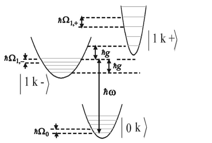
Figure 2: Energy level diagram

We notice that the level spacings of the three sets of dressed vibronic states are not equal, due to the $\pm g\sqrt{n}$ term in the vibronic frequency.

II Intensity-Intensity Correlations

We next consider the second-order intensity correlation function $g^{(2)}(\tau)=\langle a^{\dagger}(0)a^{\dagger}(\tau)a(\tau)a(0)\rangle/{\langle a^{\dagger}a\rangle}^{2}_{SS}$.

In the weak field limit, only states with 2 or fewer quanta of energy are left within the basis (we must keep states with at least two photons, as we wish examine photon coincidences). The limit we are considering is one in which $Y\rightarrow 0$; and we truncate our equations of motion to lowest order in $Y$. If no driving field were applied, the atom would certainly be in the ground state, so we make the approximation that for weak fields $C_{0,l,g}\sim 1$. With no trapping potential, one would have $C_{g,0}=1.0$; here we must specify the set of initial populations which correspond to the center of mass motion of the atom, subject to the normalization condition $\sum_{l}|C_{0,l,g}|^{2}=1.0$. The potential is taken to be of the same sign for plus and minus dressed states, which is possible by placing the lattice field at a “magic ”frequency magic1 ; magic2 ; magic3 .The driving field is responsible for populating the atom’s excited states, and thus $C_{1,l,\pm}\sim YC_{0,l,g}\sim Y$. This reasoning can be continued and we determine that our scaling should be

$$C_{0,l,g} \sim 1$$

$$C_{1,l,\pm} \sim Y$$

$$C_{2,l,\pm} \sim {Y}^{2}.$$ (8)

In the weak field limit, the one excitation amplitudes satisfy

$$\dot{C}_{1,l,+} = -\left({{\gamma}\over{4}}+{{\kappa}\over 2}+i\Delta_{l,1+}\right)C_{1,l,+}-{Y\over{\sqrt{2}}}C_{0,l,g}$$ (9)

$$-\left({{\gamma}\over{4}}-{{\kappa}\over 2}\right)C_{1,l,-}$$

$$\dot{C}_{1,l,-} = -\left({{\gamma}\over{4}}+{{\kappa}\over 2}+i\Delta_{l,1-}\right)C_{1,l,-}-{Y\over{\sqrt{2}}}C_{0,l,g}$$ (10)

$$-\left({{\gamma}\over{4}}-{{\kappa}\over 2}\right)C_{1,l,+}$$

with $\Delta_{1,l\pm}=\left(\Omega_{1,\pm}-\Omega_{0}\right)l\pm g$, recall the effective harmonic frequency

$$m\Omega_{n\pm}^{2}=\alpha\pm{{\hbar g_{m}\sqrt{n}}\over{\eta^{2}}}.$$ (11)

and again, we keep only lowest order terms in the driving field $Y$. These are the frequencies that correspond to the energy levels of the system, the $\alpha$ term arises from the external potential, the $\pm g\sqrt{n}$ terms from the spatial structure of the cavity mode function and the coupling of motion in the mode to the interaction with the driving field.

As a first step we note that we can solve the equations of motion for the slowly varying population amplitudes $\dot{D}_{n,k,\pm,}$, defined as

$$D_{0,l,g} = C_{0,l,g},$$

$$D_{1,l,\pm} = C_{1,l,\pm}e^{-it(\Omega_{1,\pm}l-\Omega_{0}l\pm g)},$$

$$D_{2,1,\pm} = C_{2,l,\pm}e^{-it(\Omega_{2,\pm}l-\Omega_{0}l\pm\sqrt{2}g)}.$$ (12)

We find that our $\dot{C}_{n,l,\pm}$ equations become

$$\dot{D}_{0,l,g} = \dot{C}_{0,l,g}\simeq 0$$

, (13)

$$\dot{D}_{1,l,+} = -\left[\frac{\gamma}{4}+\frac{\kappa}{2}+i(\Omega_{1,+}l-\Omega_{0}l+g)\right]D_{1,l,+}$$

$$- \frac{Y}{\sqrt{2}}D_{0,l,g}$$

$$- \left[\frac{\gamma}{4}-\frac{\kappa}{2}\right]D_{1,l,-},$$

$$\dot{D}_{1,l,-} = -\left[\frac{\gamma}{4}+\frac{\kappa}{2}+i(\Omega_{1,-}l-\Omega_{0}l-g)\right]D_{1,l,-}$$

$$+ \frac{Y}{\sqrt{2}}D_{0,l,g}$$

$$- \left[\frac{\gamma}{4}-\frac{\kappa}{2}\right]D_{1,l,+},$$

$$\dot{D}_{2,l,+} = -\left[\frac{\gamma}{4}+\frac{3\kappa}{2}+(i(\Omega_{2,+}l-\Omega_{0}l+\sqrt{2}g)\right]D_{2,l,+}$$

$$- Y\left[\frac{1}{\sqrt{2}}+\frac{1}{2}\right]D_{1,l,+}$$

$$+ Y\left[\frac{1}{\sqrt{2}}-\frac{1}{2}\right]D_{1,l,-}$$

$$- \left[\frac{\gamma}{4}-\frac{\kappa}{2}\right]D_{2,l,-},$$

$$\dot{D}_{2,l,-}= - \left[\frac{\gamma}{4}+\frac{3\kappa}{2}+(i(\Omega_{2,-}l-\Omega_{0}l-\sqrt{2}g)\right]D_{2,l,-}$$

$$+ Y\left[\frac{1}{\sqrt{2}}-\frac{1}{2}\right]D_{1,l,+}$$

$$- Y\left[\frac{1}{\sqrt{2}}+\frac{1}{2}\right]D_{1,l,-}$$

$$- \left[\frac{\gamma}{4}-\frac{\kappa}{2}\right]D_{2,l,+}.$$

In the weak field limit, these equations have a steady state solution

$$|\Psi_{ss}\rangle=\sum_{n,l}\left(D_{n,l,+}^{ss}|n,l,+\rangle+D_{n.l,-}|n,l,-\rangle\right)$$ (18)

The system reaches this steady state, which has a very small average photon number, $\langle a^{\dagger}a\rangle\sim Y^{2}\ll 1$. In any given time step $\Delta t$ the probability of a collapse is given by $P_{cav}=2\kappa\langle a^{\dagger}a\rangle\Delta t\ll 1$. Similarly the probability of a spontaneous emission event in a time step $\Delta t$, $P_{atom}=\gamma\langle\sigma_{+}\sigma_{-}\rangle\Delta t$ is small. Eventually there is a cavity emission, or a spontaneous emission by the atom, leaving the system in the states

$$|\Psi_{c}\rangle=\left\{\begin{array}[]{r@{\quad:\quad}l}a|\Psi_{ss}\rangle=\frac{|\Psi_{CT}(0)\rangle}{||\Psi_{CT}(0)\rangle|^{2}}&Transmission\\ \sigma_{-}|\Psi_{ss}\rangle=\frac{|\Psi_{CF}(0)\rangle}{||\Psi_{CF}(0)\rangle|^{2}}&Flourescence\end{array}\right..$$ (19)

In the steady state, all population amplitudes $D_{n,k,\pm}$ are constant, and we may set all $\dot{D}_{n,k,\pm}=0$. Equations II and II then become

$$\left(\begin{array}[]{cc}\frac{\gamma}{4}+\frac{\kappa}{2}+i(\Omega_{1,+}l-\Omega_{0}l+g)&\frac{\gamma}{4}-\frac{\kappa}{2}\\ \frac{\gamma}{4}-\frac{\kappa}{2}&\frac{\gamma}{4}+\frac{\kappa}{2}+i(\Omega_{1,-}l-\Omega_{0}l-g)\\ \end{array}\right)\left(\begin{array}[]{c}D^{ss}_{1,l,+}\\ D^{ss}_{1,l,-}\\ \end{array}\right)=\left(\begin{array}[]{c}\frac{-Y}{\sqrt{2}}\\ \frac{Y}{\sqrt{2}}\\ \end{array}\right)D^{ss}_{0,l,g}.$$ (20)

Solving for $D^{ss}_{1,l,+}$ and $D^{ss}_{1,l,-}$, we find

$$D^{SS}_{1,l,+} = \frac{A_{l}(G+H_{l})}{F_{l}H_{l}-G^{2}},$$

$$D^{SS}_{1,l,-} = \frac{-A_{l}(G+F_{l})}{F_{l}H_{l}-G^{2}},$$ (21)

where

$$A_{l} = \frac{Y}{\sqrt{2}}D_{0,l,g},$$

$$G = -\left[\frac{\gamma}{4}-\frac{\kappa}{2}\right],$$

$$H_{l} = -\left[\frac{\gamma}{4}+\frac{\kappa}{2}+i(\Omega_{1,-}l-\Omega_{0}l-g)\right],$$

$$F_{l} = -\left[\frac{\gamma}{4}+\frac{\kappa}{2}+i(\Omega_{1,+}l-\Omega_{0}l+g)\right].$$ (22)

Using the same procedure, we may use our results for $D^{ss}_{1,l,+}$ and $D^{ss}_{1,l,-}$ and solve equations (II) and (II) for $D^{ss}_{2,l,+}$ and $D^{ss}_{2,l,-}$, finding

$$D^{SS}_{2,l,+} = \frac{-G\beta_{2,l}-Z_{l}\beta_{1,l}}{G^{2}-Y_{l}Z_{l}},$$

$$D^{SS}_{2,l,-} = \frac{-G\beta_{1,l}-Y_{l}\beta_{2,l}}{G^{2}-Y_{l}Z_{l}}.$$ (23)

where

$$Y_{l} = \frac{\gamma}{4}+\frac{3\kappa}{2}+i(\Omega_{2,+}l-\Omega_{0}l+\sqrt{2}g),$$

$$Z_{l} = \frac{\gamma}{4}+\frac{3\kappa}{2}+i(\Omega_{2,-}l-\Omega_{0}l-\sqrt{2}g),$$

$$\beta_{1,l} = -Y\left[\frac{1}{\sqrt{2}}+\frac{1}{2}\right]D^{SS}_{1,l,+}+Y\left[\frac{1}{\sqrt{2}}-\frac{1}{2}\right]D^{SS}_{1,l,-},$$

$$\beta_{2,l} = +Y\left[\frac{1}{\sqrt{2}}-\frac{1}{2}\right]D^{SS}_{1,l,+}-Y\left[\frac{1}{\sqrt{2}}+\frac{1}{2}\right]D^{SS}_{1,l,-}.$$ (24)

Now that the steady state values for the population amplitudes have been calculated, our task is to solve for the time evolution of $D_{1,l,+}(t)$ and $D_{1,l,-}(t)$. The probability of a cavity emission at time $\tau$ given that one occurred at $\tau=0.0$ is $2\kappa\langle\Psi_{CT}|a^{\dagger}a|\Psi_{CT}\rangle\Delta t$, hence we have

$$g^{(2)}_{TT}(\tau) = {{\langle\Psi_{CT}|a^{\dagger}a|\Psi_{CT}\rangle}\over{\langle\Psi_{SS}|a^{\dagger}a|\Psi_{SS}\rangle}}$$ (25)

$$= {{\sum_{n,l}n|C_{g,n,1}^{CT}(\tau)|^{2}}\over{\sum_{n,l}n|C_{g,n,l}^{SS}|^{2}}}$$

$$= {{\sum_{l}|C_{g,1,l}^{CT}|^{2}(\tau)}\over{\sum_{l}|C_{g,1,l}^{SS}|^{2}}}$$

where we have truncated the results to lowest order in the weak field limit. Similarly we have for the second order intensity correlation function for the fluorescent field is given by

$$g^{(2)}_{FF}(\tau) = {{\langle\Psi_{CF}|\sigma_{+}\sigma_{-}|\Psi_{CF}\rangle}\over{\langle\Psi_{SS}|\sigma_{+}\sigma_{-}|\Psi_{SS}\rangle}}$$ (26)

$$= {{\sum_{n,l}n|C_{e,n,1}^{CF}(\tau)|^{2}}\over{\sum_{n,l}n|C_{e,n,l}^{SS}|^{2}}}$$

$$= {{\sum_{l}|C_{e,0,l}^{CF}|^{2}(\tau)}\over{\sum_{l}|C_{e,0,l}^{SS}|^{2}}}$$

To facilitate solving the time evolution of the one-excitation amplitudes we write them in matrix form as

$$\dot{\vec{A}}(t)=M\vec{A}(t)+\vec{\Delta},$$ (27)

where

$$\vec{A}(t) = \left(\begin{array}[]{c}{D}_{1,l,+}(t)\\ {D}_{1,l,-}(t)\\ \end{array}\right),$$ (30)

$$M = \left(\begin{array}[]{cc}-\left[\frac{\gamma}{4}+\frac{\kappa}{2}+i(\Omega_{1,+}l-\Omega_{0}l+g)\right]&-\left[\frac{\gamma}{4}-\frac{\kappa}{2}\right]\\ -\left[\frac{\gamma}{4}-\frac{\kappa}{2}\right]&-\left[\frac{\gamma}{4}+\frac{\kappa}{2}+i(\Omega_{1,-}l-\Omega_{0}l-g)\right]\\ \end{array}\right),$$ (33)

$$\vec{A}(t) = \left(\begin{array}[]{c}{D}_{1,l,+}(t)\\ {D}_{1,l,-}(t)\\ \end{array}\right),$$ (36)

$$\vec{\Delta} = \frac{Y}{\sqrt{2}}\left(\begin{array}[]{c}-1\\ 1\\ \end{array}\right)D_{0,l,g}.$$ (39)

The form of the time evolution of $D_{1,l,+}(t)$ and $D_{1,l,-}(t)$:

$$\vec{A}(t)=\left(Se^{\Lambda t}S^{-1}\right)\vec{A}(0)+\left(Se^{\Lambda t}S^{-1}-1\right)M^{-1}\vec{\Delta}.$$ (40)

Without showing the details of such calculations, we arrive at

$$D_{1,l,+}(t) = \left[\frac{{\beta_{2}}^{\prime}}{2{\chi}_{2}}D_{1,l,+}(0)+\frac{G}{2{\chi}_{2}}D_{1,l,-}(0)+\frac{YD_{0,l,g}}{2{\chi}_{2}\phi\sqrt{2}}\left[-H_{l}{\beta}_{2}^{\prime}+G^{2}-G{\beta}_{2}^{\prime}+GF_{l}\right]\right]e^{\lambda_{1}t}$$ (41)

$$+ \left[\frac{{-\beta_{1}}^{\prime}}{2{\chi}_{2}}D_{1,l,+}(0)-\frac{G}{2{\chi}_{2}}D_{1,l,-}(0)+\frac{YD_{0,l,g}}{2{\chi}_{2}\phi\sqrt{2}}\left[H_{l}{\beta}_{1}^{\prime}-G^{2}+G{\beta}_{1}^{\prime}-GF_{l}\right]\right]e^{\lambda_{2}t}$$

$$+ \left[\frac{H_{l}+G}{\phi}\frac{Y}{\sqrt{2}}\right]D_{0,l,g},$$

$$D_{1,l,-}(t) = \left[\frac{{-\beta_{1}}^{\prime}}{2{\chi}_{2}}D_{1,l,-}(0)-\frac{\beta_{1}^{\prime}\beta_{2}^{\prime}}{2G{\chi}_{2}}D_{1,l,+}(0)+\frac{YD_{0,l,g}}{2{\chi}_{2}\phi\sqrt{2}}\left[\frac{H_{l}}{G}\beta_{1}^{\prime}\beta_{2}^{\prime}-G\beta_{1}^{\prime}+\beta_{1}^{\prime}\beta_{2}^{\prime}-\beta_{1}^{\prime}F_{l}\right]\right]e^{\lambda_{1}t}$$ (42)

$$+ \left[\frac{{\beta_{2}}^{\prime}}{2{\chi}_{2}}D_{1,l,-}(0)+\frac{\beta_{1}^{\prime}\beta_{2}^{\prime}}{2G{\chi}_{2}}D_{1,l,+}(0)+\frac{YD_{0,l,g}}{2{\chi}_{2}\phi\sqrt{2}}\left[-\frac{H_{l}}{G}\beta_{1}^{\prime}\beta_{2}^{\prime}+G\beta_{2}^{\prime}-\beta_{1}^{\prime}\beta_{2}^{\prime}+\beta_{2}^{\prime}F_{l}\right]\right]e^{\lambda_{2}t}$$

$$- \left[\frac{F_{l}+G}{\phi}\frac{Y}{\sqrt{2}}\right]D_{0,l,g},$$

where

$$\chi_{1} = \frac{F_{l}+H_{l}}{2},$$

$$\chi_{2} = \frac{\sqrt{(F_{l}-H_{l})^{2}+4G^{2}}}{2},$$

$$\lambda_{1} = \chi_{1}+\chi_{2},$$

$$\lambda_{2} = \chi_{1}-\chi_{2},$$

$$\beta_{1}^{\prime} = F_{l}-\lambda_{1},$$

$$\beta_{2}^{\prime} = F_{l}-\lambda_{2},$$

$$\phi = F_{l}H_{l}-G^{2}.$$ (43)

We are now equipped with all the necessary information to solve for the dynamics of our system in the weak field limit.

For the rest of the paper, we restrict ourselves to the deep trapping limit, where $\alpha\geq g_{m}\sqrt{n}/\lambda^{2}$. We may then use the binomial approximation, and define

$$\Omega_{n,\pm}\approx\sqrt{\frac{\alpha}{m}}\left[1\pm\frac{\hbar mg_{m}\sqrt{n}}{2\eta^{2}\alpha}\right],$$ (44)

therefore we find $\Delta_{n,\pm}=\Omega{n,\pm}-\Omega_{0}$ for $n=1,2$ to be

$$\Delta_{1,+} = \frac{\hbar g_{m}\sqrt{n}}{2\eta^{2}\sqrt{m\alpha}},$$

$$\Delta_{1,-} = -\Delta_{1,+},$$

$$\Delta_{2,+} = \sqrt{2}\Delta_{1,+},$$

$$\Delta_{2,-} = -\sqrt{2}\Delta_{1,+}.$$ (45)

and we can characterize everything by the one detuning $\Delta_{1,+}$. This is analogous to the Lamb-Dicke regime in an ion trap.

By using the well dressed states, we have a set of equations that will have a steady-state. Recall that the quantum number $l$ is associated with a well-dressed state, and not simply the vibrational quantum number of the lattice potential. To solve these equations it is necessary to specify the amplitudes, $C_{g,0,1}(0)$ that are each of order unity. They can be related to the initial center of mass state of the atom via $C_{g,0,l}=\langle g,0,l|\psi\rangle=\int\phi_{g,0,l}^{*}\Psi(x)dx$ , or simply specified.

For weak driving fields, the probability of a cavity emission in a time $\Delta t$ is given by $P_{cav}=2\kappa\langle a^{\dagger}a\rangle\Delta t$ is quite small, as is the probability of a spontaneous emission, $P_{spon.em.}=\gamma\langle\sigma_{+}\sigma_{-}\rangle\Delta t$. In this case the wave function attains a steady state $|\psi\rangle_{SS}=\sum\limits_{n,l=0}^{\infty}\left[{C_{1,l,+}^{SS}e^{-iE_{1,l,+}t}|1,l,+\rangle+C_{1,l,-}^{SS}e^{-iE_{1,l,-}t}|1,l,-\rangle}\right]$.

After a photon is detected in transmission, at $t=0$ the wave function collapses to

$$|\psi(0)\rangle_{Coll} = a|\psi\rangle_{SS}/|a|\psi\rangle_{SS}|$$ (47)

$$= \sum\limits_{n,l=0}^{\infty}\left(C_{g,n,l}^{Coll}(t)e^{-iE_{g,n,l}t}|g,n,l\rangle\right.$$

$$\left.+C_{e,n,l}^{Coll}(t)e^{-iE_{e,n,l}t}|e,n,l\rangle\right)$$

. The initial value of the one-photon amplitudes of the collapsed state are related to the steady state two-photon amplitudes

$$C_{g,1,l}^{Coll}(0) = {{\sqrt{2}C_{g,2,l}^{SS}}\over{\sum_{n,l}\left[2{\mid C_{g,2,l}^{SS}\mid}^{2}+{\mid C_{e,1,l}^{SS}\mid}^{2}\right]}}$$ (48)

$$C_{e,0,l}^{Coll}(0) = {{C_{e,1,l}^{SS}}\over{\sum_{n,l}\left[2{\mid C_{g,2,l}^{SS}\mid}^{2}+{\mid C_{e,1,l}^{SS}\mid}^{2}\right]}}$$ (49)

and these are found above.

The relation between the well dressed probability amplitudes and the bare amplitudes is

$$D_{n,l,\pm}={1\over{\sqrt{2}}}(C_{e,n-1,l}\pm C_{g,n,l})$$ (50)

Before turning to our results, let us recall the relations that $g^{(2)}(\tau)$ must satisfy if the field can be described by a classical stochastic process; if it has a positive definite Glauber-Sudarshan P distribution,

$$g^{(2)}(0) \geq 1$$ (51)

$$g^{(2)}(0+) \geq g^{(2)}(0)$$ (52)

$$|g^{(2)}(\tau)-1| \leq |g^{(2)}(\tau)-1|$$ (53)

Violations of all three of these inequalities has been observed in CQED systems expt1 ; expt2

III Results for intensity correlations

As the system has a steady-state wave function in the steady state, we may write

$$g^{(2)}(\tau)={{\langle\Psi_{C}(\tau)|a^{\dagger}a|\Psi_{C}(\tau)\rangle}\over{\langle a^{\dagger}a\rangle_{SS}}}.$$ (54)

where we define

$$|\psi_{C}\rangle={{a|\psi_{SS}\rangle}\over{|a|\psi_{SS}\rangle|}}={{a|\psi_{SS}\rangle}\over{\sqrt{\langle|\psi_{SS}|a^{\dagger}a|\psi_{SS}\rangle|}}}$$ (55)

In Fig. 3 we plot $g^{(2)}(0)-1$ for an initial state $\mid\Psi_{g}\rangle$ where there is equal population in the $\mid 0,l,g\rangle$ states for $l=0,l_{max}$. As more states are involved, we find that the antibunching goes away. This is due to the fact that the two single-photon vibronic ladders have a different frequency spacing than the ground state vibronic levels, and is consistent with the effect of detunings on the photon statisticsthy . Involving more $l$ states makes the width of the state larger, increasing $\Delta x$ for the center of mass wave function of the atom. The antibunching also goes away if we just prepare the system in a particular higher $l$ state $\mid 0,l_{0},g\rangle$. The optimum state would seem to be the ground state of the bare vibronic potential.

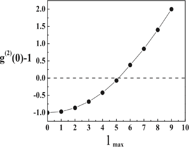
Figure 3: $g^{(2)}(0)-1$ vs. $N_{max}$, the highest occupied phonon number

Instead of just assigning values to the probability amplitudes (subject to normalization) we can specify the center of mass wave function and calculate the probability amplitudes via $D_{g,0,1}(0)=\langle\Psi_{CM}|l\rangle$. If we choose the center of mass wave function to be a Gaussian of width $\sigma$, we can calculate these amplitudes easily using

$$D_{g,0,l} = \langle\Psi_{CM}|l\rangle$$ (56)

$$= A_{n,l}\int^{\infty}_{\infty}e^{-y^{2}/2\sigma^{2}}e^{-y^{2}/2\sigma_{0}^{2}}H_{l}(y)dy$$

where $y=x/\sigma_{0}$ and $\sigma_{0}=\sqrt{\hbar/m\Omega_{0,l}}$ is the width of the ground state of the vibronic potential, and the normalization constant is $A_{n,l}=(m\Omega_{0,l}/\pi\hbar)^{1/4}/\sqrt{2^{n}n!}$.

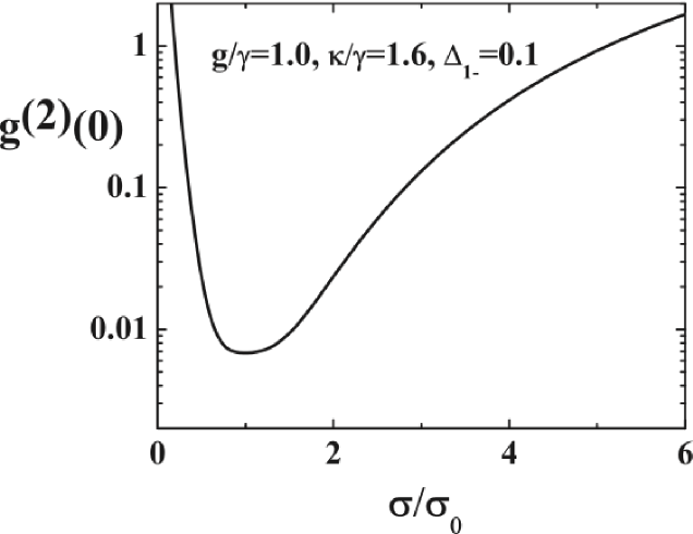
Figure 4: $g^{(2)}(0)-1$ vs. $\sigma/\sigma_{0}$, the relative width of a Gaussian center of mass wave function

In Fig. 4 we show a plot of $g^{(2)}(0)$ as a function of $\sigma/\sigma_{0}$ for parameters for which there is nearly perfect antibunching in the absence of an external potential. We see that there is a relatively wide region where the antibunching persists, but for $\sigma/\sigma_{0}$ less than $0.2$ or larger than $4$, the antibunching vanishes completely. This can be understood by considering that a Gaussian wave function is superposition of various vibronic states, and that population of higher excited vibronic states is deleterious to antibnching. Only when $\sigma/\sigma_{0}\approx 1$ do we have a center of mass wave function that has population predominantly in the ground state In Fig. 5, we show a plot of $g^{(2)}(\tau)$ for $g/\gamma=2$, $\kappa/\gamma=5$, $\Delta_{1,+}/\gamma=0.1$. Fig. 5a is for the atom initially in the ground state of the potential. We see that $g^{(2)}(0)$ is about $1.1$. Classically, $g^{(2)}(\tau)$ could not then go below $0.9$, but here it goes to zero. We refer to this as an undershoot. In Fig. 5b, we exhibit $g^{(2)}(\tau)$ for an equal admixture of the ground state and fifth excited state. Here $g^{(2)}(0)$ is $4$, and hence the fact that $g^{(2)}(\tau)$ is later zero is not nonclassical. The physical reason for this can be traced back to the fact that an atom in an excited state of the external potential is essentially detuned from resonance. With $\Delta_{1,+}/\gamma=0.1$, the detuning $\Delta_{5,+}/\gamma=0.5$. Previous work has shown that usually a detuning of half a linewidth is quite deleterious to nonclassical effects in $g^{(2)}(\tau)$. In Fig. 5c, we have results for what we refer to as a pseudo-Boltzmann. Here we populate 20 vibronic levels of the external potential at a ”temperature” of 3mK. There is no decoherence associated with this distribution, i.e. all the off-diagonal matrix elements are not zero. This essentially results in a distribution over populations with small population in the first excited state,even less in the second, and so on. Here we see that with most of the population in the ground state, we essentially have the ground state result. In Fig. 5d, we show $g^{(2)}(\tau)$ for an equal population in all $20$ vibronic states. Here we see large photon bunching, and no nonclassical effects at all. This can be understood in terms of detunings of the various atomic states; this type of distribution over vibronic states would correspond to an atom more localized than the ground state of the external potential. Hence we see that localizing the atom too much results in a large spread in momentum states that destroys the nonclassical effects.

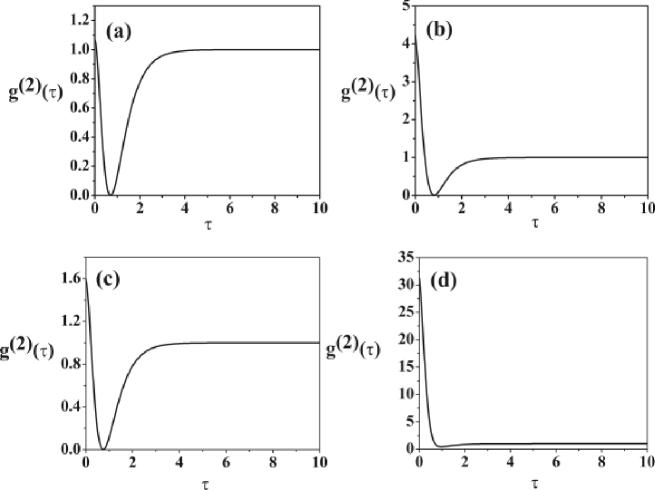
Figure 5: Plots are $g_{TT}^{(2)}(\tau)$ for $g/\gamma=2$, $\kappa/\gamma=5$, $\Delta_{1,+}/\gamma=0.1$, and (a) $|0\rangle$ only, (b) $\frac{1}{\sqrt{2}}\left[|0\rangle+|5\rangle\right]$, (c) Pseudo-Boltzmann, and (d) for 20 states with equal population.

In Fig. 6, we see that the fluorescent intensity correlations are relatively insensitive to the choice of atomic center of mass wave function, in that $g^{(2)}(0)$ is $0$ due to the nature of single-atom fluorescence.

Figure 6: Plots are $g_{FF}^{(2)}(\tau)$ for $g/\gamma=2$, $\kappa/\gamma=5$, $\Delta_{1,+}/\gamma=0.1$, and (a) $|0\rangle$ only, (b) $\frac{1}{\sqrt{2}}\left[|0\rangle+|5\rangle\right]$, (c) Pseudo-Boltzmann, and (d) for 20 states with equal population.

In Fig. 7 we examine $g^{(2)}(\tau)$ for parameters where the transmitted intensity correlation function $g^{(2)}(0)=0.0$. We see that for a superposition of ground and fifth excited states, we still have nonclassical effects, as $g^{(2)}(0)\leq 1$. The initial slope of $g^{(2)}(\tau)$ is negative though, which is not nonclassical. For the pseudo-Boltzmann distribution, we see both types of nonclassical behaviors. In the case of equal population over 20 vibronic states, there is no nonclassical behavior at all.

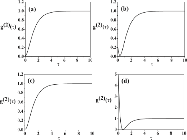
Figure 7: Plots are $g_{TT}^{(2)}(\tau)$ for $g/\gamma=2.2$, $\kappa/\gamma=10$, $\Delta_{1,+}/\gamma=0.1$, and (a) $|0\rangle$ only, (b) $\frac{1}{\sqrt{2}}\left[|0\rangle+|5\rangle\right]$, (c) Pseudo-Boltzmann, and (d) for 20 states with equal population.

In Fig. 8, we look at a case where there is strong coupling, but no nonclassical behavior in the ground state case. We do have strong vacuum-Rabi oscillations. For an admixture of states, we see a beat frequency in the oscillations. The pseudo-Boltzmann case again is very similar to the ground state case. The oscillations are almost completely washed out when we have equal population in 20 vibronic states.

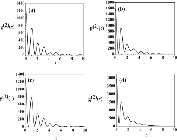
Figure 8: Plots are $g_{TT}^{(2)}(\tau)$ for $g/\gamma=3$, $\kappa/\gamma=.1$, $\Delta_{1,+}/\gamma=0.1$, and (a) $|0\rangle$ only, (b) $\frac{1}{\sqrt{2}}\left[|0\rangle+|5\rangle\right]$, (c) Pseudo-Boltzmann, and (d) for 20 states with equal population.

In Fig. 9 we again look at a situation where the ground state case shows strong vacuum-Rabi oscillations as well as all three nonclassical behaviors; $g^{(2)}(0)\leq 1$, the initial slope is positive, and there is an overshoot violation. The latter refers to $g^{(2)}(\tau)$ violating the upper limit of the inequality in 53.

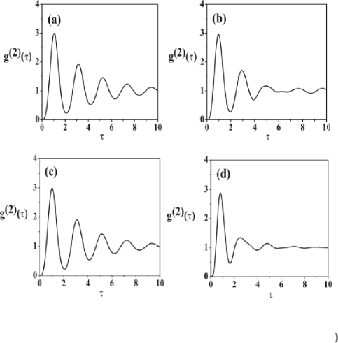
Figure 9: Plots are $g_{FF}^{(2)}(\tau)$ for $g/\gamma=3$, $\kappa/\gamma=.1$, $\Delta_{1,+}/\gamma=0.1$, and (a) $|0\rangle$ only, (b) $\frac{1}{\sqrt{2}}\left[|0\rangle+|5\rangle\right]$, (c) Pseudo-Boltzmann, and (d) for 20 states with equal population.

In Fig. 10 we have a situation where we only have an overshoot violation in the ground state case. This violation vanishes in the case of a superposition of ground and fifth excited state, as well as for an equal population of 20 vibronic states. In Figure 11, we examine the effects of increasing spacing between the vibronic levels. To this point we have dealt with detunings on the order of $0.1$ linewidths.

Figure 10: Plots are $g_{TT}^{(2)}(\tau)$ for $g/\gamma=1$, $\kappa/\gamma=.77$, $\Delta_{1,+}/\gamma=0.1$, and (a) $|0\rangle$ only, (b) $\frac{1}{\sqrt{2}}\left[|0\rangle+|5\rangle\right]$, (c) Pseudo-Boltzmann, and (d) for 20 states with equal population.

In Fig. 12 we can see that increasing the detunings allows us to see a larger effect due to the beat frequency. Changing the detuning to $0.3$ and $0.5$ of $\gamma$, we see that the initial slope is not nonclassical, but we still have $g^{(2)}(0)\leq 1$, and there is an undershoot violation. So the nature of the nonclassicality is not changed. At a detuning of $2.0$, we still have an undershoot violation as well as evidence of oscillations at the beat frequency.

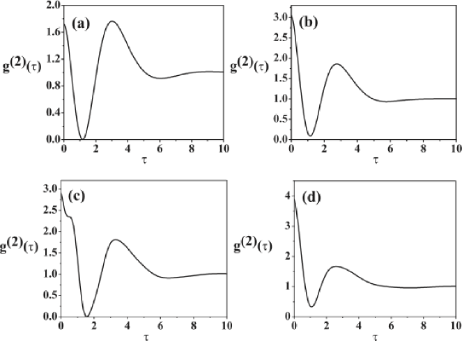
Figure 11: Plots are $g_{TT}^{(2)}(\tau)$ for $g/\gamma=1$, $\kappa/\gamma=1.6$. All trials use $\frac{1}{\sqrt{2}}\left[|0\rangle+|5\rangle\right]$ as the vibrational state distribution with (a) $\Delta_{1,+}/\gamma=0.1$, (b) $\Delta_{1,+}/\gamma=0.3$, (c) $\Delta_{1,+}/\gamma=2.0$, (d) $\Delta_{1,+}/\gamma=0.5$.

In Figure 12, we examine the effects of increasing spacing between the vibronic levels. In this case we have antibunching, a violation of inequality in Eq.(51). Changing the $\Delta_{1,+}/\gamma$ to $0.3$ and $0.5$, we see that the initial slope is not nonclassical, but we still have $g^{(2)}(0)\leq 1$, and there is an undershoot violationexpt2 . So the nature of that nonclassicality is not changed. At a detuning of $2.0$,(Fig. 5c) we still have an undershoot violation as well as evidence of oscillations at the beat frequency.

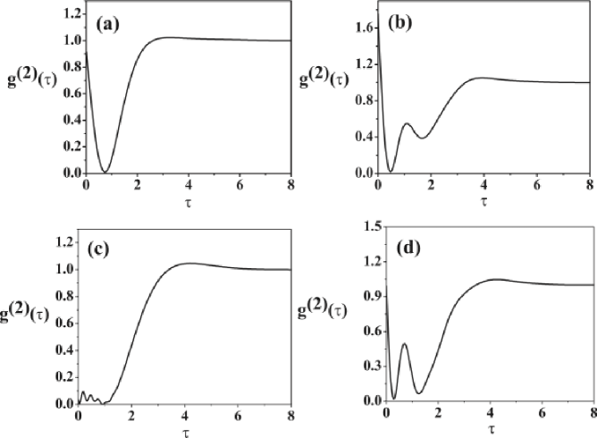
Figure 12: Plots are $g_{TT}^{(2)}(\tau)$ for $g/\gamma=1$, $\kappa/\gamma=1.6$. All trials use $\frac{1}{\sqrt{2}}\left[|0\rangle+|5\rangle\right]$ as the vibrational state distribution with (a) $\Delta_{1,+}/\gamma=0.1$, (b) $\Delta_{1,+}/\gamma=0.3$, (c) $\Delta_{1,+}/\gamma=2.0$, (d) $\Delta_{1,+}/\gamma=0.5$.

IV Wave-Particle Correlations

Recently, Carmichael his co-workers have introduced a new intensity-field correlation function $h_{\theta}(\tau)$ that is of great interest HT1 ; HE1 . Because $h_{\theta}(\tau)$ is an intensity-field correlation function, it takes the general form

$$h_{\theta}(\tau)={{\langle I(0)E(\tau)\rangle}\over{\langle I\rangle\langle E\rangle}},$$ (57)

and for a quantized field, this becomes

$$h_{\theta}(\tau)={{\langle{a}^{\dagger}(0)a_{\theta}(\tau)a(0)\rangle}\over{\langle{a}^{\dagger}a\rangle\langle a_{0}\rangle}},$$ (58)

where we have, like for $g^{(2)}(\tau)$, exploited normal and time ordering, and we have used the quantum mechanical field quadrature operator :

$${a}_{\theta}={1\over 2}\left(ae^{-\imath\theta}+{a}^{\dagger}e^{\imath\theta}\right).$$ (59)

In Eq. (59), $\theta$ is the phase of the local oscillator (LO) with respect to the average signal field. We see that with the $a$ acting to the right, and the ${a}^{\dagger}$ acting to the left at $t=0$, a collapsed state is prepared, the collapse being a photon loss from the field, corresponding to a detection event. Then at $t=\tau$ one measures $\langle a_{\theta}\rangle$ conditioned on the previous detection. This differs from a direct measurement of $\langle a_{\theta}\rangle$ with no conditioning. An ensemble average of the latter measurements (necessary to get a good signal to noise ratio) would yield zero due to phase fluctuations. The conditioned BHD measurement essentially looks at members of the ensemble with the same phase, a phase that is set by the photodetection.

As with other correlation functions, like the second-order intensity correlation function $g^{(2)}(\tau)$, restrictions can be placed on $h_{\theta}(\tau)$ if there is an underlying positive definite probability distribution function for amplitude and phase of the electric field, i.e. that the field is classical albeit stochastic. By ignoring third-order moments (a Gaussian fluctuation assumption that is valid for weak fields), one finds

$$h_{\theta}(\tau)=1+2{{\langle:\Delta{a}_{\theta}(0)\Delta{a}_{\theta}(\tau):\rangle}\over{\langle\Delta{a}^{\dagger}\Delta{a}\rangle}},$$ (60)

and we see that the intensity-field correlation function is connected to the spectrum of squeezing HT1

$$S_{\theta}(\omega)\propto\int_{0}^{\infty}d\tau\cos(\omega\tau)\left[h_{\theta}(\tau)-1\right].$$ (61)

From this, it has been shown that the Schwartz inequality would yield

$$0\leq h_{\theta}(0)-1\leq 1,\\$$ (62)

and more generally

$$\mid h_{\theta}(\tau)-1\mid\leq\mid h_{\theta}(0)-1\mid\leq 1.$$ (63)

Whenever there is squeezing, these inequalities do not hold for $h_{\theta}(\tau)$. Giant violations of these inequalities have been predicted for an optical parametric oscillator, and a group of $N$ atoms in a driven optical cavity, and have been recently observed in the cavity QED system HE1 .

Now consider the following quantity

$$\langle IE\rangle^{2}\leq\langle I\rangle^{2}\langle E\rangle^{2}$$ (64)

After some algebra we find

$$h^{2}_{0}(0) = {{\langle IE\rangle^{2}}\over{\langle I\rangle^{2}\langle E\rangle^{2}}}$$ (65)

$$\leq {{\langle I^{2}\rangle\langle E^{2}\rangle}\over{\langle E\rangle^{2}\langle I\rangle^{2}}}$$

$$\leq {{\langle I\rangle}\over{\langle E\rangle^{2}}}g^{(2)}(0)$$

$$\leq g^{(1)}(0)g^{(2)}(0)$$ (66)

In the absence of an external potential $g^{(2)}(0)=|C_{g,1}^{CT}/C_{g,1}^{ss}|^{2}=h^{2}_{0}(0)$. As $h_{0}(0)$ will be nonclassical above $2$, we must have bunching to see nonclassical behavior in the conditioned fields. Also in the system considered here , we would have $h^{2}\leq g^{(2)}$; when we include an optical lattice we have

$$h_{0}(0) = {{\sum_{k}C^{c}_{1,g,k}}\over{\sum_{k}C^{ss}_{1,g,k}}}$$ (67)

$$g^{(2)}(0) = {{\sum_{k}|C^{c}_{1,g,k}|^{2}}\over{\sum_{k}|C^{ss}_{1,g,k}|^{2}}}$$ (68)

$$|h_{0}(0)|^{2} = {{|\sum_{k}C^{c}_{1,g,k}|^{2}}\over{|\sum_{k}C^{ss}_{1,g,k}|^{2}}}$$ (69)

Just looking at the numerator, for two vibronic modes k values, we would violate Eq. (66).

As with $g^{(2)}(\tau)$, we obtain an analytic solution using the quantum trajectory method, and again we look at weak driving fields. We find

$$\langle{a}^{\dagger}(0)a_{\theta}(\tau)a(0)\rangle=\langle\psi_{c}\mid a_{\theta}\mid\psi_{c}\rangle,$$ (70)

where $\mid\psi_{c}\rangle$ is the collapsed state produced by the photodetection event, as in the case of $g^{(2)}(\tau)$. Once again we need only keep the states with two or less excitations (total in the cavity mode or internal energy) for weak driving fields. The result is that

$$h_{\theta}(\tau) = {{\langle n\rangle_{SS}\langle{a}_{\theta}(\tau)\rangle_{CT}}\over{{\langle n\rangle_{SS}\langle{a}_{\theta}(\tau)\rangle_{SS}}}}$$ (71)

$$= {{\langle{a}_{\theta}(\tau)\rangle_{CT}}\over{\langle{a_{0}(\tau)\rangle_{SS}}}}.$$

The expectation value of the field quadrature operator is given by

$$\langle{a}_{\theta}\rangle=\sum_{n,l}\left(\sqrt{n}C^{*}_{n,l}C_{n-1,l}e^{-\imath\theta}+\sqrt{n+1}C^{*}_{n,l}C_{n+1,l}e^{\imath\theta}\right).$$ (72)

In the weak field limit we have

$$\langle{\hat{a}}_{\theta}\rangle=\sum_{l}\left(C^{*}_{1,l}C_{0,l}e^{-\imath\theta}+C^{*}_{0,l}C_{1,l}e^{\imath\theta}\right).$$ (73)

So finally then, for weak fields we have

$$h_{\theta}(\tau)=\frac{\sum_{l}\left(C^{CT}_{1,l}C^{CT}_{0,l}e^{-\imath\theta}+{C^{CT}}^{*}_{0,l}C^{CT}_{1,l}e^{\imath\theta}\right)}{\sum_{l}\left(C^{SS*}_{1,l}C^{SS}_{0,l}+C^{SS*}_{0,l}C^{SS}_{1,l}\right)}.$$ (74)

For the fluorescent field, we have

$$h_{\theta}^{FF}(\tau)={{\langle\sigma_{\theta}(\tau)\rangle_{CF}}\over{\langle\sigma_{0}(\tau)\rangle_{SS}}}.$$ (75)

which in terms of probability amplitudes is

$$h_{\theta}^{FF}(\tau)={{2Re{\sum_{l}C^{CF}_{0,e,l}(\tau)C_{0,g,l}^{CF}(\tau)}e^{i\theta}}\over{{\sum_{l}C^{SS}_{0,e,l}C_{0,g,l}^{SS}}}}.$$ (76)

In Fig. 14 we plot $h_{\theta}^{TT}$ for $g/\gamma=2$, $\kappa/\gamma=5$, for the same choice of four states we have used. We see that in the case of a highly localized atom (equal probability of 20 vibronic levels) the nonclassical nature of $h_{\theta}^{TT}$ is actually enhanced. In the case of an admixture of ground and fifth excited states, the behavior of $h_{\theta}^{TT}$ is relatively unchanged from the ground state case. This is due to the insensitivity of $h_{\theta}^{TT}$ to detunings in the weak coupling limit. In the strong coupling regime, as shown in Fig. 15, we see the same general behavior, although for the case of 20 equal populations we do see some dephasing of the vacuum-Rabi oscillations, due to the detunings of the various levels involved. Similar behavior is seen in the case of $h_{\theta}^{FF}$ as shown in Figs. 16 and 17. Note that $h_{\theta}^{FF}(0)=0.0$, reflecting the fact that after spontaneous emission, the dipole field envelope vanishes. In Fig. 18 we change the level spacing. We see that for increasing vibronic level spacing the nature of the nonclassicality persists, but there is evidence of the beat frequency between subsequent vibronic levels.

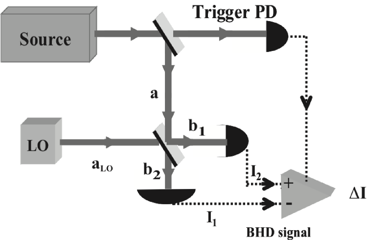
Figure 13: This is a common experimental setup for measuring $h_{\theta}(\tau)$. In this figure, the source would be either the transmitted or fluoresced portion of the field. LO denotes Local Oscillator, a

Figure 14: Plots are $h^{TT}_{\theta}(\tau)$ for $g/\gamma=2$, $\kappa/\gamma=5$ , $\Delta_{1,+}/\gamma=0.1$. (a) $|0\rangle$ only. (b) $\frac{1}{\sqrt{2}}\left[|0\rangle+|5\rangle\right]$. (c) Pseudo-Boltzmann. (d) All states equal population.

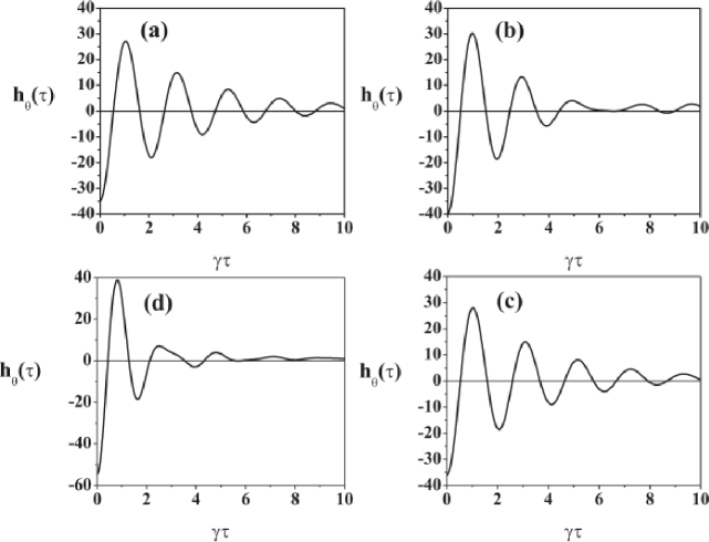
Figure 15: Plots are $h^{TT}_{\theta}(\tau)$ for $g/\gamma=3$, $\kappa/\gamma=.1$ , $\Delta_{1,+}/\gamma=0.1$. (a) $|0\rangle$ only. (b) $\frac{1}{\sqrt{2}}\left[|0\rangle+|5\rangle\right]$. (c) Pseudo-Boltzmann. (d) All states equal population.

Figure 16: Plots are $h^{TT}_{\theta}(\tau)$ for $g/\gamma=3$, $\kappa/\gamma=.1$ , $\Delta_{1,+}/\gamma=0.1$. (a) $|0\rangle$ only. (b) $\frac{1}{\sqrt{2}}\left[|0\rangle+|5\rangle\right]$. (c) Pseudo-Boltzmann. (d) All states equal population.

Figure 17: Plots are $h^{FF}_{\theta}(\tau)$ for $g/\gamma=1$, $\kappa/\gamma=.77$ , $\Delta_{1,+}/\gamma=0.1$. (a) $|0\rangle$ only. (b) $\frac{1}{\sqrt{2}}\left[|0\rangle+|5\rangle\right]$. (c) Pseudo-Boltzmann. (d) All states equal population.

Figure 18: Plots are $h^{TT}_{\theta}(\tau)$ for $g/\gamma=1$, $\kappa/\gamma=.77$ , $\Delta_{1,+}/\gamma=0.1$. (a) $|0\rangle$ only. (b) $\frac{1}{\sqrt{2}}\left[|0\rangle+|5\rangle\right]$. (c) Pseudo-Boltzmann. (d) All states equal population.

V Conclusion

We have considered the photon statistics of a cavity QED system while including quantized center of mass motion along the cavity axis. In the limit of weak driving fields we have found analytic results for intensity correlations of the transmitted and fluorescent fields; as well as for the cross-correlations between the transmitted and fluorescent intensities. We find that for intensity correlations for the transmitted field, having a significant population outside the ground vibronic level is deleterious to sub-Poissonian statistics, photon antibunching, and overshoot/undershoot violations. This is explained due to the sensitivity of these nonclassical effects to detunings between the atom-cavity system and the driving field. It is found that significant population in vibronic levels that are out of resonance by a half a linewidth is sufficient to severely modify the results; a highly localized atom, spread over many vibronic levels only exhibits nonclassical effects over a very small parameter range. For the fluorescent intensity correlations, we do not find such a sensitivity, this is due mainly to the nature of single atom fluorescence where the atom can only emit one photon at a time. The cross-correlations exhibit the assymetry noted by Denisov et. al., and this asymmetry is not degraded significantly by a distribution over vibronic levels.

We have also found analytic results for $h_{\theta}(\tau)$ for the transmitted and fluorescent fields. There is no time asymmetry for weak driving fields. The nonclassical behavior in $h_{\theta}(\tau)$ is not generally degraded by a distribution over vibronic levels; indeed it is sometimes enhanced.

Future work includes inclusion of 2- and 3-d external trapping potentials, non-harmonic potentials, and pressing beyond the weak field limit.

References

(1) For a comprehensive review, see Optical Coherence and Quantum Optics, L. Mandel
and E. Wolf, Cambridge (2000).
(2)E.T. Jaynes and F.W. Cummings, Proc. IEEE 51, 89 (1963).
(3)Cavity Quantum Electrodynamics, edited by P. Berman, in Advances
in Atomic and Molecular Physics, Supplement 2, Academic, San
Diego, (1994), Any other good reviews that are
later??.
(4)H. J. Carmichael, R. J. Brecha, and P. R. Rice,
Optics Communications 82, 73 (1991);R. J. Brecha, P. R.
Rice, and X. Min, Phys. Rev. A 59, 2392 (1999).
(5) G. Rempe, R. J. Thompson, R. J. Brecha, W. D. Lee, and H. J. Kimble
Phys. Rev. Lett. 67, 1727 (1991)
(6)G. T.
Foster, S. L. Mielke, and L. A. Orozco Phys. Rev. A 61,
053821 (2000).
(7) A nice introduction is L Guidoni and P Verkerk, J.
Opt. B 1, R23 (1999).
(8)J. McKeever, A. Boca, A. D. Boozer, J. R. Buck, and H. J.
Kimble, Nature (London) 425, 268 (2003).
(9) H. J. Carmichael, An Open Systems Approach To Quantum Optics, (Springer-Verlag, Berlin, 1993), L. Tian and H. J. Carmichael, Phys. Rev. A. 46, R6801 (1992).
(10) D. W. Vernooy and H. J. Kimble
Phys. Rev. A 56, 4287-4295 (1997)
(11) C. J. Hood and C. Wood, as described by H. J. Kimble et al., in Laser Spectroscopy XIV, edited by Rainer Blatt et al. (World Scientific, Singapore, 1999), p. 80.
(12)H. Katori, T. Ido and M., Kuwata-Gonokami, J. Phys. Soc. Jpn. 68, 2479 (1999), T. , Y. Isoya, and H. Katori, Phys. Rev. A 61, 061403 (2000).
(13) S. J. van Enk, J. McKeever, H. J. Kimble, and J. Ye, Phys. Rev. A 64 013407 (201).
(14)H. J. Carmichael, H. M.Castro-Beltran, G. T. Foster, and L. A.
Orozco, Phys. Rev. Lett. 85, 1855 (2000).
(15)G. T. Foster, L. A. Orozco, H. J. Carmichael, and H. M.
Castro-Beltran, Phys. Rev. Lett. 85, 3149 (2000).