Constructing smooth potentials of mean force, radial distribution functions and probability densities from sampled data

Abstract

In this paper a method of obtaining smooth analytical estimates of probability densities, radial distribution functions and potentials of mean force from sampled data in a statistically controlled fashion is presented. The approach is general and can be applied to any density of a single random variable. The method outlined here avoids the use of histograms, which require the specification of a physical parameter (bin size) and tend to give noisy results. The technique is an extension of the Berg-Harris method [B.A. Berg and R.C. Harris, Comp. Phys. Comm. 179, 443 (2008)], which is typically inaccurate for radial distribution functions and potentials of mean force due to a non-uniform Jacobian factor. In addition, the standard method often requires a large number of Fourier modes to represent radial distribution functions, which tends to lead to oscillatory fits. It is shown that the issues of poor sampling due to a Jacobian factor can be resolved using a biased resampling scheme, while the requirement of a large number of Fourier modes is mitigated through an automated piecewise construction approach. The method is demonstrated by analyzing the radial distribution functions in an energy-discretized water model. In addition, the fitting procedure is illustrated on three more applications for which the original Berg-Harris method is not suitable, namely, a random variable with a discontinuous probability density, a density with long tails, and the distribution of the first arrival times of a diffusing particle to a sphere, which has both long tails and short-time structure. In all cases, the resampled, piecewise analytical fit outperforms the histogram and the original Berg-Harris method.

I Introduction

In many situations the probability to find a particle at a certain distance from a given other particle is of interest. This probability is given by the radial distribution function. In addition to providing detailed information on the local structure of a system, one can often express thermodynamic quantities such as the pressure, energy and compressibility in terms of the radial distribution functions.McQuarrie Furthermore, the radial distribution function can be reformulated in terms of a potential of mean force, which is of great importance in multi-scale simulations that take the potential of mean force as input in Langevin or Brownian dynamics simulations.FrenkelSmit ; Berendsen07

Radial distribution functions are usually constructed in simulations by forming a histogram of sampled inter-particle distances. FrenkelSmit However, histograms contain the bin size as a free parameter, and can be rather noisy for a poorly selected value of this parameter. For probability densities, an alternative method recently proposed by Berg and Harris avoids histograms and yields a smooth analytical form for the probability density which describes the sample data statistically at least as well as the noisy histogram.BergHarris08 This method has already proved useful in the context of the computation of quantum free energy differences from non-equilibrium work distributions,VanZonetal08b the determination of the density in Bose-Einstein condensates, Gerickeetal08 and in the distribution of a reaction coordinate in simulations of chemical reactions.Monesetal09

Having a similar method for potentials of mean force and radial distribution functions would have many advantages. As in the Berg-Harris method, such an approach would avoid the noise that accompanies the standard histogram method, while no a priori choice of bin size is required. Furthermore, a smooth radial distribution would give a better representation of the potential of mean force (which is related to the logarithm of the radial distribution function), and allows the function to be evaluated at any point in the range over which it is defined. Finally, the expressions for the pressure, energy and compressibility in terms of the radial distribution functions involve integrals of the radial distribution function over $r$. Such integrals can be evaluated more accurately from an analytic form than from a histogram, whose accuracy is restricted by the bin size.

The purpose of this paper is to develop an approach to obtain smooth radial distribution functions and potentials of mean force from sampled inter-particle distances. The resulting method turns out to be suitable not just for radial distribution functions and potentials of mean force, but for a large class of densities of single random variables.

The paper is structured as follows. Sec. II presents a model of water in which rigid molecules interact through a discretized potential. Construction of radial distribution functions from data derived from this model will be used as a running test case. This section also contains some details on the generation of sampled data through simulation. The Berg-Harris method for smoothing probability densities in a statistically controlled fashion, and the connection between probability distribution functions and radial distribution functions, are briefly reviewed in Sec. III. In Sec. IV, simulation results are presented that show the shortcoming of the Berg-Harris method for radial distribution functions. The extended method is developed in Sec. V, with Sec. V.1 containing an explanation for the poor performance and its solution through statistical resampling. Sec. V.2 addresses an additional problem related to the particular shape of radial distribution functions, which is solved by extending the method to use piecewise analytic functions. In Sec. VI, the generality of the method is illustrated by presenting the results of applying the method to data drawn from three different probability densities which are problematic for the original Berg-Harris method. The paper concludes with a discussion in Sec. VII.

II System: a discrete water model

In the development of the smooth approximation method below, a model of rigid water molecules subject to a discretized interaction potential between the molecules will be used as a running test case for the construction of radial distribution functions. Since a water molecule consists of two kinds of atoms (oxygen and hydrogen), there are three radial distribution functions in this system, $g_{\mathrm{OO}}$, $g_{\mathrm{OH}}$ and $g_{\mathrm{HH}}$, which turn out to have quite different character and therefore give a more stringent test of the smooth fitting methods than a single-atom model would.

The relative distances between the atomic sites in molecules are fixed, making the molecules rigid bodies. Each state of each body $i$ can therefore be described by its center-of-mass position $\mathbf{r}_{i}$, its orientation or attitude matrix $\mathsf{A}_{i}$ that transforms coordinates from the lab frame to a body-fixed frame for molecule $i$, and the associated linear and angular momenta. Here the body-fixed frame is chosen so that the third row of the matrix $\mathsf{A}_{i}$ corresponds to the direction of the molecule’s dipole $\bm{\mu}_{i}$, whose magnitude is fixed at a value $\mu$.

The interaction potential between a pair of molecules $i$ and $j$ is a discrete version of the soft sticky dipole potential LiuIchiye95 ; ChandraIchiye99 ; Tanetal03 ; FennellGezelter04

$$v_{ij}=v^{\mathrm{LJ}}(\mathbf{r}_{i}-\mathbf{r}_{j})+v^{\mathrm{dp}}(\mathbf{r}_{i}-\mathbf{r}_{j},\mathsf{A}_{i},\mathsf{A}_{j})+v^{\mathrm{sp}}(\mathbf{r}_{i}-\mathbf{r}_{j},\mathsf{A}_{i},\mathsf{A}_{j}),$$ (1)

where the Lennard-Jones, dipole, and sticky parts of the potential are, respectively, given by

$$v^{\mathrm{lj}}(\mathbf{r}) = 4\epsilon\left[\left(\frac{\sigma}{r}\right)^{12}-\left(\frac{\sigma}{r}\right)^{6}\right]$$ (2)

$$v^{\mathrm{dp}}(\mathbf{r},\mathsf{A}_{i},\mathsf{A}_{j}) = \frac{\bm{\mu}_{i}\cdot\bm{\mu}_{j}}{r^{3}}-\frac{\bm{\mu}_{i}\cdot\mathbf{r}\ \bm{\mu}_{j}\cdot\mathbf{r}}{r^{5}}$$ (3)

$$v^{\mathrm{sp}}(\mathbf{r},\mathsf{A}_{i},\mathsf{A}_{j}) = \frac{v_{0}}{2}\Bigg{[}s(r)\{\sin\theta_{ij}\sin 2\theta_{ij}\cos 2\phi_{ij}$$ (4)

$$\qquad\quad+\sin\theta_{ji}\sin 2\theta_{ji}\cos 2\phi_{ji}\}$$

$$\quad+s^{\prime}(r)\{(\cos\theta_{ij}-0.6)^{2}(\cos\theta_{ij}+0.8)^{2}$$

$$\qquad\qquad+(\cos\theta_{ji}-0.6)^{2}(\cos\theta_{ji}+0.8)^{2}$$

$$\qquad\qquad-2\omega^{0}\}\Bigg{]}$$

where $\theta_{ij}$ and $\phi_{ij}$ are the conventional spherical angles of the vector $\mathsf{A}_{i}\mathbf{r}$, and $\theta_{ji}$ and $\phi_{ji}$ are those of $\mathsf{A}_{j}\mathbf{r}$. Finally, the switching function $s(r)$ is defined as

$$s(r)=\left\{\begin{array}[]{ll}1&\mbox{ for }r<r_{L}\\ \frac{(r_{U}-r)^{2}(r_{U}+2r-3r_{L})}{(r_{U}-r_{L})^{3}}&\mbox{ for }r_{L}<r<r_{U}\\ 0&\mbox{ for }r>r_{U}\end{array}\right.,$$ (5)

while $s^{\prime}(r)$ is given by the same form with primed parameters $r^{\prime}_{L}$ and $r^{\prime}_{U}$.

Here, the so-called SSD/E reparameterization of the model was used, for which the parameter values are $\epsilon=0.152$ kcal/mol, $\sigma=3.035$ Å, $\mu=2.42$ D, $v_{0}=3.90$ kcal/mol, and $\omega^{0}=0.07715$, while the cut-off parameters in the functions $s$ and $s^{\prime}$ are taken to be $r_{L}=2.4$ Å, $r_{U}=3.8$ Å, $r_{L}^{\prime}=2.75$ Å and $r_{U}^{\prime}=3.35$ Å.FennellGezelter04

The discontinuous interaction potential in our system is obtained from the smooth potential by the controlled energy discretization method presented in Ref. VanZonSchofield08, . In this discretization, a cut-off naturally arises, and therefore no reaction field was included.

The natural simulation technique for systems with discretized potentials is discontinuous molecular dynamics, or DMD. dmd1 ; dmd2 ; VanZonSchofield08 In DMD, the dynamics of the system is free (no forces or torques are present) in between interaction events at which linear and angular momenta change. By its very nature, the energy-discretization scheme used in DMD is symplectic, time-reversible and strictly conserves the total (discretized) energy. It has no fixed time-step, but moves from event to event. The event frequency, which sets the efficiency of the method to a large degree, is determined by the level of discretization of the potential energy: the finer the discretization, the more events occur. One typically finds that a discretization of the order of $\frac{1}{2}k_{B}T$ already suffices for a reasonably accurate simulation of the smooth system.VanZonSchofield08 In the simulations of which the results are presented below, the discretization of the potential energy was set to $\frac{1}{4}k_{B}T$.

The orientational dynamics of free rigid bodies is an important aspect in the calculation of interaction times.dmd1 ; dmd2 The solution of the equations of motion for the angular momenta and attitude matrix $\mathsf{A}$ depends on the symmetry of the body through the principal moments of inertia. Although any value of the principal moments can be utilized to sample configurations of a system of rigid molecules, the DMD simulations presented here made use of the exact solution of the equations of motion for a free, asymmetric rigid rotor,dmd1 ; VanZonSchofield07a and hence were based on the exact dynamics of the system.

At the time of a distance measurement in the simulation, the forces and torques are most likely zero, since these quantities are non-zero only at discrete time points. This makes alternative smoothing methods, such as the weighted residual methodCyrBond07 and methods based on equilibrium identities using (smooth) forces,AdibJarzynski05 ; BasnerJarzynski08 not applicable here. Since only the inter-particle distances are available as input for the determination of the analytically-fitted radial distribution functions, the comparison with histogram-based radial distribution functions is more equitable.

III Review

III.1 Smoothing probability densities with the Berg-Harris method

Consider a random variable $r$ which has a probability density $p(r)$. Suppose that one has a sample of $n$ data points $\{r_{i}\}$ that are independently drawn from the density $p(r)$. How can one estimate $p(r)$ from the data points? One way is to bin the data points into a histogram. Because histograms are quite sensitive to statistical noise, Berg and Harris developed the following alternative procedure to obtain an analytical estimate for the probability density from the data.BergHarris08

In the Berg-Harris method, the data are first sorted such that $r_{i}<r_{i+1}$. Using the sorted data, the empirical cumulative distribution function $\bar{F}$ is defined in the range $[r_{1},r_{n}]$ as

$$\bar{F}(r)=\frac{i}{n}\qquad\mbox{for $r_{i}\leq r<r_{i+1}$}.$$ (6)

Although $\bar{F}$ becomes a better approximation to the true cumulative distribution $F(r)=\int^{r}p(r^{\prime})\,dr^{\prime}$ with increasing sample size $n$, it is a function with many steps for any finite value of $n$ so that its derivative is not analytic but rather consists of delta functions.

The next step consists of writing the function $\bar{F}$ as a sum of a linear term and a Fourier expansion. The expansion is truncated at the $m$th term:

$$\bar{F}(r)\approx F_{m}(r)\equiv F_{0}(r)+\sum_{j=1}^{m}d_{j}\sin[j\pi F_{0}(r)],$$ (7)

where the linear term is defined as

$$F_{0}(r) = \frac{r-r_{1}}{r_{n}-r_{1}}.$$ (8)

Furthermore, the Fourier coefficients $d_{j}$ in Eq. (7) are determined from

$$d_{j}=\frac{2}{r_{n}-r_{1}}\int_{r_{1}}^{r_{n}}[\bar{F}(r)-F_{0}(r)]\sin[j\pi F_{0}(r)]\>dr.$$ (9)

When $\bar{F}$ is approximated by $F_{m}$, the probability density $p$ is approximately

$$p_{m}(r)=\frac{1}{r_{n}-r_{1}}\left\{1+\pi\sum_{j=1}^{m}d_{j}j\cos[j\pi F_{0}(r)]\right\}.$$ (10)

Because $\bar{F}-F_{0}$ is zero at the end points of the interval $[r_{1},r_{n}]$, and the Fourier modes form a complete orthonormal basis of the space of such functions, the empirical cumulative distribution $\bar{F}$ and the associated probability density are reconstructed exactly by Eqs. (7) and (10) as $m\to\infty$. However, as mentioned above, this limit would yield a series of delta functions for the probability density $\bar{p}=p_{\infty}$. The aim is to truncate the series at a level $m$ which is not too high that one is fitting the noise, but high enough to give a good smooth approximation to $\bar{F}$ and $\bar{p}$.

The final step of the procedure is therefore to find the appropriate number of Fourier terms $m$ in a statistically controlled fashion. The value of $m$ is determined here using the Kolmogorov-Smirnov (K-S) test.BergHarris08 ; NumRecipes This test determines how likely it is that the difference between the empirical cumulative distribution function $\bar{F}$ and its analytical approximation $F_{m}$ is due to noise.footnote1 The test takes the maximum variation $D_{m}$ between $\bar{F}$ and $F_{m}$ over the sampled points ($D_{m}=\max_{i=1\dots n}|F_{m}(r_{i})-\bar{F}(r_{i})|$), and returns a probability $Q_{m}=Q(D_{m})$ that the difference between the two cumulative distribution functions is due to chance. The functional dependence of $Q$ on $D$ is known to a good (asymptotic) approximation.Stephens70

A small value of $Q_{m}$ indicates that the difference between the cumulative distribution functions is statistically significant, i.e. the quality of the expansion $F_{m}$ is insufficient to represent the data. One therefore carries out a process of progressively increasing the number of Fourier modes $m$ and evaluating $F_{m}$ as well as $Q_{m}$ until the value of $Q_{m}$ is larger than some convergence threshold $Q_{\mathrm{cut}}$. A reasonable value for this convergence value is $Q_{\mathrm{cut}}=0.6$.

In Ref. VanZonetal08b, , errors were estimated using the jackknife algorithm,Efron79 and the same method will be used here. However, since the inter-particle distance data naturally come in blocks, each corresponding to a single configuration, not all data points are independent. To account for this, we use a block-version of the jackknife method, in which a single block of data is omitted in each jackknife sample.Kuensch89

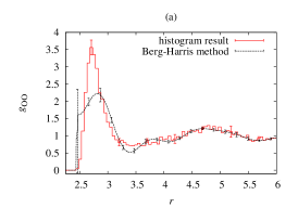
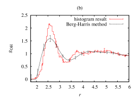
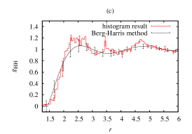
Figure 1: Performance of the straightforward application of the Berg-Harris smoothing methods applied to the radial distribution functions $g_{\mathrm{OO}}$ (a), $g_{\mathrm{OH}}$ (b), and $g_{\mathrm{HH}}$ (c) of the discretized water model. For comparison, the results from the histogram method are also shown (with error bars representing 95% confidence intervals at selected points). Here the range over which the radial distribution functions are analyzed is defined to be $[0,L/2]$, with $L/2=12.4$ Å

III.2 From probability densities to potentials of mean force

To be able to apply the above smoothing method to radial distributions, for which histograms are presently the method of choice, one has to make the connection between a probability density on the one hand, and the radial distribution function and potentials of mean force on the other hand. This connection will be briefly reviewed here because some of the details are needed below.

Consider a system of a single type of particle, in which the number of particles is $N$ and the volume of the system is $V$. The radial distribution function, denoted by $g(r)$, is the density of particles at a distance $r$ away from a chosen first particle relative to the mean density $N/V$. The true density at a distance $r$ from a first particle is thus $(N/V)g(r)$. The mean number of particles at a distance between $r$ and $dr$ from a given particle is then $n(r)=(N/V)g(r)4\pi r^{2}dr$. The Jacobian factor $4\pi r^{2}$, which is, of course, the surface area of a sphere with radius $r$, will play an important role below. The probability of a particle being at a distance $r$ is equal to the number of particles with this $r$, divided by the total number of particles, $N$, i.e. $p(r)dr=n(r)/N=g(r)4\pi r^{2}dr/V$, so one has the relation

$$g(r)=\frac{V}{4\pi r^{2}}\,p(r).$$ (11)

Systems with different types of particles give rise to different radial distribution functions $g_{ij}(r)$, where $i$ and $j$ label the kinds of particles. A similar argument to that above leads to the relation,

$$g_{ij}(r)=\frac{V}{4\pi r^{2}}\,p_{ij}(r),$$ (12)

where $p_{ij}(r)$ is the probability density of distances between a particle $j$ and a particle $i$. Once $g_{ij}(r)$ is known, the potential of mean force $\Phi_{ij}$ is found fromMcQuarrie

$$\Phi_{ij}(r)=-k_{B}T\ln g_{ij}(r),$$ (13)

where $T$ is the temperature of the system and $k_{B}$ is Boltzmann’s constant.

A further consideration for the applicability of the Berg-Harris method to radial distribution functions is whether the K-S test may be used at all. The K-S test assumes that the samples are independently drawn. Correlation between the samples may result in a bias in the radial distribution functions. Since nearby particles in an instantaneous configuration of the system are correlated, this is potentially an issue. If, however, the system is sufficiently large, only a small fraction of the samples in a single configuration will be spatially correlated, making the K-S test applicable to a very good approximation. Furthermore, if one ensures that the configurations are taken from the simulation at sufficiently large time intervals, time correlations do not pose a problem either.

IV Poor performance of the straightforward smoothing applied to radial distribution functions

Using the Berg-Harris method to get a smooth probability densities $p(r)$ from a sample of inter-particle distances, one expects to obtain a good, smooth fit to $g(r)$ by using Eq. (12). To test this expectation, the system of pure water in which rigid water molecules interact via a discretized potential energy derived from the soft sticky dipole model described in Sec. II was simulated. For all simulation results presented in this section, the parameters of the water model were as follows. The temperature is set at $T=298~{}\rm K$, the number of particles is $N=512$, the cubic simulation box has sides of length $L=24.8$Å, so that the density is $1.0$ kg$/$l. The principal moments of inertia of a rigid water molecule are $I_{x}=0.0337365\,m_{H_{2}O}$Ų, $I_{y}=0.0635040\,m_{\mathrm{H_{2}O}}$Ų, and $I_{z}=0.0972405\,m_{\mathrm{H_{2}O}}$Ų, where $m_{\mathrm{H_{2}O}}$ is the molecular mass of water. After equilibration, the simulations were run for $8$ picoseconds, in which the inter-particle distances were sampled every $2$ picoseconds (long enough for the system to decorrelate), for a total of $4$ configurations.

From these data, the radial distributions $g_{\mathrm{OO}}$, $g_{\mathrm{OH}}$ and $g_{\mathrm{HH}}$ were determined in the simulations through histograms and by following the smoothing procedure of Sec. III.1, using a value for $Q_{\mathrm{cut}}$ of $0.6$. The results for the three radial distribution functions are shown in Fig. 1. Clearly, the two methods do not agree very well at short inter-particle separations, despite the fact that the smooth distance distributions are statistically good descriptions of the distance data according to the K-S test. In particular, note that the peak heights defining the first solvation shell are not well-described.

V Extending the Berg-Harris method

Given these unsatisfactory results, the histogram method would be preferred over the straightforward application of the Berg-Harris method. But there is a way to fix the smoothing method to the extent that the smoothing method becomes preferable over the histogram method. To understand how to fix the problem, one first needs to understand its underlying causes.

V.1 Over-represented large distances

V.1.1 Problematic Jacobian

The convergence criterion of the smooth approximation relies on the K-S test.BergHarris08 ; NumRecipes This test is based only on the maximum variation $D_{m}$ between $\bar{F}$ and $F_{m}$ and is more sensitive to typical data points than to outliers. Although this may appear to be a contradiction at first glance, it is important that the K-S test depends on the maximum deviation in the cumulative distribution function, rather than on the deviation of the random variable from the mean. To see that outliers do not constitute very deviant points in the cumulative distribution, suppose that, by chance, an outlier $x_{out}$ from the far left tail of a distribution is found in a sample of size $n$. This would yield an increase of magnitude of $1/n$ for the empirical cumulative distribution $\bar{F}$ at $x_{out}$, while the cumulative distribution $F(x)$ is practically zero since $x$ is in the region where the distribution is very small. If $F_{m}$ is not too bad an approximation to $F$, $\bar{F}-F_{m}$ will also be of order $1/n$ at $x_{out}$. However, the deviation between $F_{m}$ and $\bar{F}$ at other points $x$ depends more on the goodness of fit than on the sample size, at least for points $x$ in regions that contain a sizable fraction of the samples: these are the ‘typical points’. For these points, there is little sample size dependence, so that to first order in $n$, one has $\bar{F}-F_{m}=O(n^{0})$. Since $O(n^{-1})<O(n^{0})$ for large enough sample sizes, the outlier $x_{out}$ will not be seen as the most deviant point in the K-S test, but rather, some typical value $x$ will have the most deviant cumulative distribution.footnote1a

The above argument holds when the quality of the fit in the typical region is poor. However, as the number of Fourier modes used to fit $\bar{F}$ is increased, the quality of the fit of the cumulative distribution $F$ improves in the typical region, and the maximum deviation shifts to less probable values. Because the probability density function is small in the tails, this maximum deviation of the distribution is not that large and the convergence criterion (the K-S test) is met, resulting in a good fit in the typical region with a poor fit in the tails.

The Berg-Harris method of Sec. III.1 therefore works well for probability densities without “long tails,” since typical values of the variable will be the values of interest. However, for radial distribution functions, the focus on typical values is the origin of the difficulties getting the straightforward Berg-Harris method to work for radial distribution functions (cf. Fig. 1). Typical values of $r$ are of no interest in radial distribution functions. In a homogeneous system such as a fluid, the typical distances between any two particles is on the order of half the system size, $L/2$. The length scales of interest in the radial distribution functions to describe local structure are typically much smaller than that.

To make this point clearer, consider a dilute gas of hard spheres with diameter $\sigma$. In the limit of infinite dilution, the radial distribution function $g(r)$ is zero for $r<\sigma$ and unity otherwise. The probability density $p(r)$ of inter-particle distances is then [cf. Eq. (11)]

$$p_{\mathrm{dilute}}(r)=\left\{\begin{array}[]{ll}0&\mbox{ for\ \ }r<\sigma\\ 4\pi r^{2}/V&\mbox{ for\ \ }r\geq\sigma.\end{array}\right.$$ (14)

Because of the Jacobian factor of $4\pi r^{2}$, the most likely values of $r$ are of the order of the largest possible $r$, which is $L/2$. This means that in a sample of inter-particle distances in the dilute hard sphere system, the large distance samples ($r_{i}=\mathcal{O}(L/2)$) are much more abundant than the small distance samples ($r_{i}=\mathcal{O}(\sigma)$). Thus, when approximating $p(r)$ by a smooth function using the K-S test, the long-distance part will be fitted very well, but the short-distance behavior ($r=\mathcal{O}(\sigma)$) will not, because the test used is sensitive to the typical values of $r$, which are $\mathcal{O}(L/2)$.

The conclusion that large distance values overwhelm the smaller ones in which one is interested is valid beyond the dilute hard sphere case, since the Jacobian factor in Eq. (14) acts on long length scales and is therefore also present in systems of higher density with non-negligible interactions.

A crude attempt at solving the large distance problem is to impose a cut-off $r_{\rm cut}$ on the allowed values of $r$ in the sample of inter-particle distances. This cut-off should be of the order of the distance over which $g(r)$ differs from one. But to determine that distance one has to measure $g(r)$. Thus, one would have to guess a value of the cut-off distance and adjust it until $g(r)$ approaches one within a certain accuracy for $r<r_{\mathrm{cut}}$. Unfortunately, even when the cut-off is chosen in this way, the results, although better than those in Fig. 1, are still not very impressive, as Fig. 2 for the oxygen-oxygen radial distribution function shows with $r_{\mathrm{cut}}$ set to $7.44$ Å(using again $Q_{\mathrm{cut}}=0.6$). One sees a lot of spurious oscillations in the smooth radial distribution functions, which are due to the high number of Fourier modes needed to fit the radial distribution function ($m=18$ in this case). Furthermore, these oscillations do not even agree within the 95% confidence interval with the histogram result, deviating especially for small distances $r$. The explanation is that the Jacobian factor $4\pi r^{2}$ in Eq. (12) is still present within the restricted sample $r<r_{\mathrm{cut}}$, and causes the peaks at larger $r$ values to be fitted better than the peaks at smaller $r$ values.

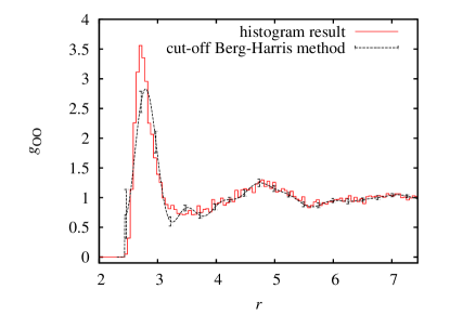
Figure 2: Result for $g_{\mathrm{OO}}$ of using a cut-off in the straightforward Berg-Harris smoothing, i.e., with the distance data restricted to $r<r_{\mathrm{cut}}=7.44$ Å. For comparison, the results from the histogram method are also shown (with error bars representing 95% confidence intervals shown at selected points).

V.1.2 Overcoming over-representation through resampling

To remove the troublesome Jacobian factor in Eqs. (11) and (12) altogether, one can resample the inter-particle distances found in the simulation. The idea is to draw from the original sample of distances, $\{r_{i}\}$ such that smaller values of $r$ are more likely than larger values by introducing a relative bias weight $w(r_{i})$ for each distance $r_{i}$ in the sample to construct a new, resampled set $\{\tilde{r}_{i}\}$.footnote1b Given that the probability densities of the original sample points is $p(r)=4\pi r^{2}g(r)/V$ [cf. Eq. (11)], and provided that subsequent resampled data points are chosen independently with weight $w(r_{i})$, the probability density of the resampled points is given by

$$\tilde{p}(r) = k^{-1}w(r)p(r)=z^{-1}r^{2}w(r)g(r),$$ (15)

where $k=\int w(r)p(r)\>dr$ and $z=kV/(4\pi)$ are constants. Note that $z$ may be determined from

$$z=\frac{V}{4\pi}\int p(r)w(r)dr=\frac{V}{4\pi}\langle{w}\rangle,$$ (16)

which may be approximated by the average of the weight over the samples:

$$\langle{w}\rangle\approx\frac{1}{n}\sum_{i=1}^{n}w(r_{i}).$$ (17)

In the application to the radial distribution functions below, we also obtained $\langle w\rangle$ from a numerical integration using the biased analytic approximation for $\tilde{p}$, the result of which differed from that given by the simpler expression in Eq. (17) by less than $0.1\%$.

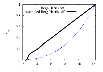
Figure 3: The resampled and the standard Berg-Harris cumulative distributions associated with the radial distribution function $g_{\mathrm{OO}}$ of the discrete water model.

The simplest way to counter the Jacobian factor $4\pi r^{2}$ in Eq. (15) is to choose a weight

$$w(r)=\frac{1}{r^{2}},$$ (18)

which gives

$$g(r)=z\tilde{p}(r),$$ (19)

with

$$z\approx\frac{4\pi}{Vn}\sum_{i=1}^{n}\frac{1}{r_{i}^{2}}.$$ (20)

In detail, the resampling leading to data with a probability density $\tilde{p}$ can be performed as follows: Given the original set $\{r_{i}\}$ one determines the weight for each data point as

$$w_{i}=w(r_{i})=\frac{1}{r_{i}^{2}}.$$ (21)

One also determines the maximum weight,

$$w_{\mathrm{max}}=\max_{i=1\dots n}w_{i}$$ (22)

to convert the weights into probabilities

$$p_{i}=\frac{w_{i}}{w_{\mathrm{max}}},$$ (23)

which, by construction, lie between 0 and 1. Next, one takes one of the original sample points $r_{i}$ at random (with equal weight), draws a random number $\xi$ uniformly from the interval [0,1] and if $\xi<p_{i}$, one adds $r_{i}$ to the resampled data set $\{\tilde{r}_{i}\}$. The procedure is repeated until enough resampled points have been gathered. There is some choice into what number of resampled points is to be taken. In our implementation, the number of resampled points is chosen to be the same as the number of points in the original sample.

Note that Eq. (19) shows that the resampled probability density $\tilde{p}$ and the radial distribution function $g$ are proportional to one another. Since $g$ approaches one for large $r$, the large values of $r$ are no longer over-represented in $\tilde{p}$.

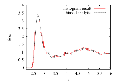
Figure 4: The radial distribution function $g_{\mathrm{OO}}$ of the discrete water model, using the resampled smoothing method described. For comparison, the results from the histogram method are also shown (with error bars representing 95% confidence intervals at selected points).

For the resampled data $\{\tilde{r}_{i}\}$, one can use the Berg-Harris smoothing method of Sec. III.1 to obtain a smooth approximation to $\tilde{p}$. Fig. 3 shows the effect of resampling on the cumulative distribution functions associated with $g_{\mathrm{OO}}$ of the water model, using $Q_{\mathrm{cut}}=0.6$. It is evident that the small-$r$ tail of the unweighted (Berg-Harris) cumulative distribution is much enhanced in the resampled cumulative distribution, and therefore more relevant to the K-S test. Note that we have plotted only the fits, and not the empirical cumulative distributions, because the fits are hard to distinguish from the empirical cumulative distributions. The differences are easier to see in the associated radial distributions, which are plotted in Fig. 4. In contrast to Fig. 2, the smooth approximation now follows the result of the histogram within error bars for the whole range of $r$ values. But like in Fig. 2, the supposedly smooth $g_{\mathrm{OO}}(r)$ exhibits fast oscillatory behavior within those error bars. This oscillatory behavior will be addressed next.

V.2 Hard-to-fit distribution functions

V.2.1 Unphysical oscillations

It is hard to reconcile the aim of having a smooth approximation to the radial distribution functions and the large number of Fourier modes needed to approximate the shape of $g(r)$, which starts out as a very flat function at small $r$, then increases sharply, reaches a maximum not far beyond this sharp rise, and then decays on a larger scale to $1$ in an oscillatory fashion. The peculiar shape of $g(r)$ leads to the oscillatory behavior seen in Figures 2 and 4. Even when the oscillations lie within error bars of the histogram results, they reintroduce a remnant of the noise similar in magnitude to that present in the histograms that one is trying to avoid.

It is conceivable that there are expansions other than the Fourier expansion that are more suitable for describing a sharply increasing function followed by a more moderate behavior. However, it is not clear at present what this specialized expansion should be. Therefore, a systematic and generic way will now be presented which avoids high-frequency modes in parts of $g(r)$ that do not require them. This will also make the method more generally applicable to discontinuous and other hard-to-fit densities.

We note that in the following section, the resampling explained in the previous section is supposed to have been performed on the data already, and that the resampled data have been sorted ($\tilde{r}_{i}\leq\tilde{r}_{i+1}$). For notational convenience, the tildes on $r$, $p$ and $F$ are omitted below.

V.2.2 Resolving the oscillation problem using a piecewise approach

The decomposition of $\bar{F}$ in Eq. (7) can be adjusted to incorporate hard-to-fit radial distributions by allowing the Fourier decomposition to be different on sub-intervals within the total interval $[r_{1},r_{n}]$. Let the full interval be divided into $k$ sub-intervals $[a_{1},a_{2}]$, $[a_{2},a_{3}]$, $[a_{3},a_{4}]$, …, $[a_{k},a_{k+1}]$, where $a_{1}=r_{1}$ and $a_{k+1}=r_{n}$. The intervals will be labelled by a Greek index, which can run from $1$ to $k$. How to choose the points $a_{\mu}$ (where $\mu=2\dots k$, with $a_{1}=r_{1}$ fixed) will be discussed later. Different intervals can have different numbers of samples that fall within its range. The fraction of the samples that fall within a given interval $\mu$ is denoted by $f_{\mu}$.

Figure 5: Illustration of a piecewise approximation $F_{0}$ to the cumulative distribution. The function $F_{0}$ (the solid line) is linear between the split points $a_{1}$, …$a_{5}$ (indicated by the dash vertical lines). The function increases by an amount $f_{\mu}$ between split points $a_{\mu}$ and $a_{\mu+1}$. The values of $a_{\mu}$ and $f_{\mu}$ used in this sketch roughly correspond to the piecewise analytic fit for the oxygen-oxygen radial distribution function, which requires $k=4$ intervals to achieve convergence.

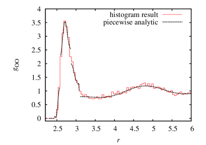
Figure 6: The radial distribution function $g_{\mathrm{OO}}$ of the discrete water model, using the first piecewise resampled smoothing method described in Sec. V.2.2. For comparison, the results from the histogram method are also shown (error bars were omitted to make the comparison clearer).

On each sub-interval, $\bar{F}(r)$ is approximated by a linear part and a truncated Fourier transform of the remainder. Analogously to Eq. (8), the linear part in interval $\mu$ is given by

$$F_{0\mu}(r)=\frac{r-a_{\mu}}{a_{\mu+1}-a_{\mu}}.$$ (24)

Note that $F_{0\mu}$ ranges from 0 to 1 in the interval $\mu$. The piecewise linear approximation to $\bar{F}$ for $r$ in interval $\mu$ is then

$$F_{0}(r)=\bar{F}(a_{\mu})+f_{\mu}F_{0\mu}(r).$$ (25)

where it should be noted that

$$\bar{F}(a_{\mu})=\sum_{\nu=1}^{\mu-1}f_{\nu}.$$ (26)

An example of such $F_{0}(r)$ is shown in Fig. 5, based on data from the oxygen-oxygen radial distribution function in the water model (as explained below). Approximations to $\bar{F}$ beyond $F_{0}$ are found by adding Fourier modes for each interval,

$$\bar{F}(r)\approx F_{0}(r)+\sum_{\mu=1}^{k}f_{\mu}\chi_{\mu}(r)\sum_{j=1}^{m_{\mu}}d_{\mu j}\sin[j\pi F_{0\mu}(r)].$$ (27)

Here, $\chi_{\mu}$ is the characteristic function on interval $\mu$, i.e.,

$$\chi_{\mu}(r)=\left\{\begin{array}[]{ll}\displaystyle 1&\mbox{ for }a_{\mu}<r<a_{\mu+1}\\ 0&\mbox{ otherwise,}\end{array}\right.$$ (28)

and $d_{\mu j}$ is given by

$$d_{\mu j}=\frac{2}{a_{\mu+1}-a_{\mu}}\int_{a_{\mu}}^{a_{\mu+1}}[\bar{F}_{\mu}(r)-F_{0\mu}(r)]\sin[j\pi F_{0\mu}(r)],$$ (29)

where

$$\bar{F}_{\mu}(r)=f_{\mu}^{-1}[\bar{F}(r)-\bar{F}(a_{\mu})].$$ (30)

The function $\bar{F}_{\mu}(r)$ is the conditional empirical cumulative probability distribution function for data points within interval $\mu$. Eq. (27) represents a piecewise analytic approximation to the cumulative distribution. Since the Fourier modes form a complete orthonormal basis, the approximation becomes exact as $m_{\mu}\to\infty$ for all $\mu$. As before, however, the $m_{\mu}$ should not become too large to avoid spurious oscillations, which only amounts to fitting the noise. One therefore defines a maximum number $m_{\mathrm{m}ax}$ of Fourier modes allowed in each sub-interval and sub-divides intervals if the maximum number of modes is not sufficient for convergence, as determined by the K-S test.

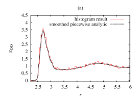
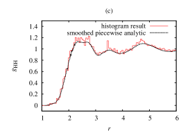
Figure 7: The resampled, piecewise-analytic method applied to the radial distribution functions $g_{\mathrm{OO}}$ (panel a), $g_{\mathrm{OH}}$ (panel b) and $g_{\mathrm{HH}}$ (panel c) of the discretized water model, using the patched piecewise resampled smoothing method. For comparison, the results from the histogram method are also shown, while error bars were omitted for clarity.

The division of the original interval is chosen dynamically as follows:

1. Start with one interval;

2. Increase $m$ until $Q>Q_{\mathrm{cut}}$;

3. If $m$ exceeds $m_{\mathrm{max}}$, find the most deviant point $a$ according to the K-S test;

4. Split the interval in two at the point $a$;

5. Repeat for the conditional distribution for each interval left and right of $a$.

Because the procedure is recursive, in each step the original one-interval procedure is used, which one exception: the allowable value of $Q$ may be set to a lower value in a sub-interval, since there are fewer points in the interval and therefore the interval carries less statistical weight. We have not found a unique, statistically controlled way to adjust the $Q_{\mathrm{cut}}$ for sub-intervals, but found heuristically that scaling the $Q_{\mathrm{cut}}$ for interval $\mu$ by $f_{\mu}$ avoids fitting the noise and leads to a satisfactory overall $Q$ value.

The recursive, multi-interval procedure is found to greatly speed up the convergence of the approximation scheme, leading to much lower $m_{\mu}$, and thus fewer oscillations. It should be stressed that splitting at the most deviant point $a$ in the K-S test is found to be essential here: choosing a different splitting point does not improve the convergence because the most deviant point is then still difficult to fit and the $Q$ value for the sub-interval containing the most deviant point remains the same.

Once the approximation in Eq. (27) has been obtained, the probability density is given by

$$p(r)\approx\frac{f_{\mu}}{a_{\mu+1}-a_{\mu}}\left\{1+\pi\sum_{j=1}^{m_{\mu}}d_{\mu j}j\cos[j\pi F_{0\mu}(r)]\right\}$$ (31)

where $\mu$ is such that $r\in[a_{\mu},a_{\mu+1}]$.

The results of applying the piecewise procedure to the $g_{\mathrm{OO}}$ of the water model are shown in Fig. 6 (remembering that $g=zp$), with $m_{\mathrm{max}}=14$ and the initial $Q_{\mathrm{cut}}$ set to $0.6$. While the method now works better than without the piecewise approach, it has one drawback: the derivative of the approximate cumulative distribution function, which gives $g(r)$, need not be a smooth function across the different intervals. As a consequence, the result in Fig. 6 shows artificial discontinuities. These discontinuities at the boundaries of the intervals fall within the 95% confidence intervals (not shown in Fig. 6).

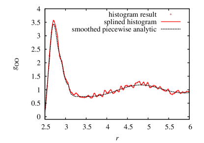
Figure 8: Comparison between the radial distribution function $g_{\mathrm{OO}}$ of the discrete water model obtained using the resampled piece-wise analytic method, and using a spline fit to the histogram results (error bars were omitted to make the comparison clearer).

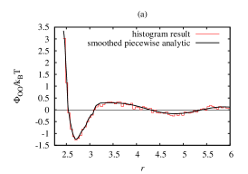
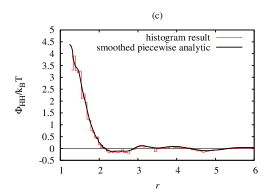
Figure 9: The resampled, piecewise-analytic method applied to the potentials of mean force $\Phi_{\mathrm{OO}}$ (panel a), $\Phi_{\mathrm{OH}}$ (panel b) and $\Phi_{\mathrm{HH}}$ (panel c) of the discretized water model. For comparison, the results from the histogram method are also shown.

V.2.3 Dealing with spurious discontinuities

Provided the underlying probability distribution of the samples is continuous, the spurious discontinuities that are present in the piecewise-analytic fit will get smaller as the number of sample points increases. Nevertheless, for cases with poor statistics, one would like to have an approach that gives a continuous piecewise analytic fit to the distribution. In fact, for some applications, having a continuous radial distribution function is essential, such as for Brownian simulations that take the potential of mean force as input. Even though the discontinuities are within the statistical noise, they would lead to sudden, unphysical changes in energy in such applications.

There are many ways to get a continuous curve out of the discontinuous one, but it should be remembered that one is working within the statistical noise. We can therefore choose any method as long as the “patch” is still statistically reasonable. To determine the statistical suitability, one can once again use the K-S test on the patched fit.

We have chosen the following simple procedure: We apply a quadratic patch function around each discontinuity at $a_{\mu}$,

$$F^{\mathrm{patch}}_{\mu}(r)=\left\{\begin{array}[]{ll}b_{\mu}[r-(a_{\mu}-c_{\mu})]^{2}&\mbox{ if }r\in[a_{\mu}-c_{\mu},a_{\mu}]\\ b_{\mu}[r-(a_{\mu}+c_{\mu})]^{2}&\mbox{ if }r\in[a_{\mu},a_{\mu}+c_{\mu}]\end{array}\right..$$ (32)

The width $c_{\mu}$ of the patch is adjustable, while the prefactor $b_{\mu}$ follows from the requirement that the cumulative distribution $F+\sum_{\mu}F^{\mathrm{patch}}_{\mu}$ has a continuous derivative at $r=a_{\mu}$. Provided the different patches do not overlap, this leads to a value of

$$b_{\mu}=\frac{\Delta p}{4c_{\mu}}.$$ (33)

where $\Delta p$ is the height of the jump in the unpatched distribution function.

Initially, each width $c_{\mu}$ is set equal to half the minimum interval size on either side of the corresponding split point $a_{\mu}$ to avoid overlap between the patches. The $Q$ value of the patched distribution is then determined, and if it is not smaller than the $Q$ value for the unpatched distribution, the patch is accepted. Otherwise, the width of the patch is reduced by a factor of two, until the $Q$ value is acceptable.footnote2 It will be demonstrated below that this solves the problem of spurious oscillations and discontinuities.

V.3 Final results

Figs. 7 show the result of the resampled, piecewise procedure for the three radial distribution functions of the water model, $g_{\mathrm{OO}}$, $g_{\mathrm{OH}}$ and $g_{\mathrm{HH}}$, with $m_{\mathrm{max}}=14$ and $Q_{\mathrm{cut}}=0.6$. It is clear that the piecewise analytic fit is now smoother than the histogram, hardly shows any oscillations and is continuous. Furthermore, while error bars were omitted in Fig. 7 for clarity, it was found that the histogram and the patched, piecewise analytic results are in mutual agreement within the 95% confidence intervals.

It may be argued that plotting the histograms using bars is an unfair way of representing the histogram results. One often takes the histograms and applies a cubic spline fitNumRecipes to the results, which makes the graph seem smoother. There is of course no a priori reason why the splined histogram should represent the radial distribution function better. For this reason, we have shown only ‘unsplined’ histograms so far. The comparison between the histograms and smooth approximations in these curves should really only be done at the mid-point of the histogram bins. Now that the piecewise analytic smoothing approach is fully developed, however, it is interesting to see how it compares to a smoothed spline fit of the histogram results. Figure 8 shows a plot of these two types of smooth results for $g_{\mathrm{OO}}$. The bin size for the histograms has been chosen such that the first peak of the radial distribution is well resolved. One sees that the cubic spline fit does a reasonable job for the first peak, but that in the second peak in the radial distribution function the spline fit is still noisy, while the statistically controlled piecewise analytic result is not. Thus, the splines cannot fix the roughness of the histogram method, at least not when bin sizes are uniform.

To show how the piecewise analytic method performs for potentials of mean force, the smooth potentials of mean force between the different species corresponding to the radial distributions in Figs. 7 [cf. Eq. (13)], have been plotted in Figs. 9. The results from the piecewise analytic method are considerably smoother than the histogram results, but still exhibit some roughness since they were based only on four configurations.

VI Further applications

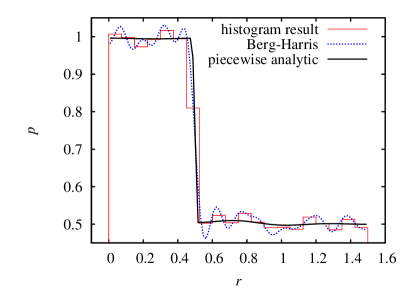
Figure 10: The piecewise-analytic method applied to $50,000$ samples drawn from the discontinuous distribution of Sec. VI.1. Also shown for comparison are the results from the histogram method and the Berg-Harris method. For clarity, error-bars on the smoothing methods and the histogram have been omitted.

The piecewise approximation method is not specific to radial distribution functions, but can help to fit any probability density that is hard to fit with a truncated Fourier series. Below, we will give several examples of such densities and show the advantages of using the piecewise analytical approximation method.

VI.1 A discontinuous density

Consider a random variable $r$ with a distribution $p$ given by

$$p(r)=\left\{\begin{array}[]{ll}0&\mbox{ if }r<0\\ 1&\mbox{ if }0<r<\frac{1}{2}\\ \frac{1}{2}&\mbox{ if }\frac{1}{2}<r<\frac{3}{2}\\ 0&\mbox{ if }r>\frac{3}{2}\end{array}\right..$$ (34)

Note that within the domain of this function $[0,\frac{3}{2}]$, there is a discontinuity at $r=\frac{1}{2}$. Discontinuities are very poorly represented by truncated Fourier series.Jeffreys

From the above distribution, 50,000 samples were drawn and used as input to the piecewise analytic approximation (with $m_{\mathrm{max}}=14$ and the initial $Q_{\mathrm{cut}}=0.6$), as well as to the one-interval analytic approximation (with the same $Q_{\mathrm{cut}}=0.6$ and unrestricted $m_{\mathrm{max}}$) and the histogram method. The results are shown in Fig. 10.

One clearly sees the trouble that the Berg-Harris one-interval approximation has in capturing the discontinuity, while the histogram is very noisy. The piecewise analytic expansion, on the other hand, beautifully captures the whole distribution; the automated procedure divides the interval $[0,\frac{3}{2}]$ in two at $r=\frac{1}{2}$ and then needs zero Fourier modes to approximate the separate pieces.

VI.2 The standard Cauchy distribution

Figure 11: The piecewise-analytic method applied to $50,000$ samples drawn from the Cauchy distribution (cf. Sec. VI.2). For comparison, the results from the histogram method and the exact result are also shown. For clarity, error-bars have been omitted. Because the piece-wise analytic result is hard to distinguish from the exact distribution, the difference between the two is plotted in Fig. 12.

According to Berg and Harris,BergHarris08 the original smoothing method has trouble with densities with long tails. It is therefore interesting to see if the piecewise approach helps for these kinds of densities as well. As an example, we consider the standard Cauchy distribution

$$p(r)=\frac{1}{\pi(1+r^{2})}.$$ (35)

From this distribution, 50,000 samples were randomly drawn and used in the piece-wise approach (with $m_{\mathrm{max}}=14$ and the initial $Q_{\mathrm{cut}}=0.6$). The results are contrasted with those of the histogram in Fig. 11. The piecewise smooth approximation performs so well that it can hardly be distinguished from the Cauchy distribution.

Not plotted in Fig. 11 were the results of the original Berg-Harris method, which, surprisingly, are so similar to the piecewise approach that they would be hard to make out in the figure. The only statistically significant difference between the two results is apparent in the height of the maximum, which the Berg-Harris fit slightly underestimates.

The success of both methods is illustrated further in Fig. 12, in which the errors in the piecewise and the one-interval results are compared; the piecewise analytic error is overall slightly smaller than that of the Berg-Harris method, but not by much. This success seems to contradict Berg and Harris’ warning against using the smoothing method for densities with long tails. It is possible the relatively high quality of the fit in the simple approach is due to the symmetric nature of the Cauchy density and its relative lack of structure.

A more stringent test of the method applied to long-tailed distributions will be presented next.

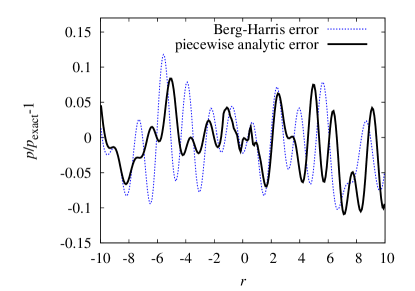
Figure 12: The error in the piecewise-analytic method applied to $50,000$ samples drawn from the Cauchy distribution (cf. Sec. VI.2) as compared to the exact form in Eq. (35). The error is here defined as the deviation from the exact result. For comparison, the errors in the Berg-Harris method are also shown.

VI.3 First arrival time distribution of a diffusing particle to a sphere

Consider a particle undergoing diffusion, starting at a distance $R_{0}$ from the origin, i.e. anywhere on a sphere of radius $R_{0}$. The distribution function $p(\mathbf{r},t)$ of the diffusing particle satisfies $\partial_{t}p=D\nabla^{2}p$, where $D$ the self-diffusion constant. Investigating the time $t$ required to arrive anywhere on the surface of a sphere of radius $R_{min}$ for the first time is a classic case of a first passage problem.Redner Such problems have applications in the rate of molecules finding each other in a solution, and are a major determining factor of reaction rates in diffusion limited reactions.

It turns out that the first arrival times are distributed according tofootnote3

$$p(t)=\frac{x}{\sqrt{4\pi Dt^{3}}}\exp\left(-\frac{x^{2}}{4Dt}\right),$$ (36)

where $x=R_{0}-R_{min}$. This distribution function has both short time structure and a long tail.

Figure 13: The piecewise-analytic method applied to $100,000$ samples drawn from the first passage time distribution of Sec. VI.3. Also shown for comparison are the results from the histogram method and the Berg-Harris method, as well as the exact result.

From the distribution in Eq. (36), 100,000 samples were randomly drawn, with parameters set at $D=1$, $R_{min}=1$ (these choices set the time and length units) and $R_{0}=10R_{min}$. The piece-wise approach was used to obtain an estimate of the probability distribution (with $m_{\mathrm{max}}=14$ and $Q_{\mathrm{cut}}=0.6$), as well as the one-interval analytic approximation ($Q_{\mathrm{cut}}=0.6$ and unrestricted $m_{\mathrm{max}}$) and the histogram method. The results are compared in Figs. 13 and 14.

While all methods work to some extent, the histogram method would have to be tailored to the function in question in order to be useful, with differently sized bins for different values of $t$. The Berg-Harris method works reasonably well without subdivisions, but exhibits fast oscillations in the tails of the density, as becomes very apparent from Fig. 14. The appearance of oscillations is not surprising when one considers that $m=390$ Fourier modes were needed for the Berg-Harris fit! The piecewise analytic result does not exhibit fast oscillations in the tail. Furthermore, the piecewise fit only required a total of 28 Fourier modes distributed over 8 intervals. Although the piecewise result does have some modulation within the error bars, we have checked that almost all of these disappear when one takes 10 times as many data points. At that level of statistics, the Berg-Harris results still have oscillations in the tails, and still require over 350 Fourier modes.

When the analytical form of $p(t)$ is not known, such as for absorption in non-spherical geometries, but samples $\{t_{i}\}$ are available from numerical simulation, the piecewise approach would give the best description of $p(t)$: one that is less noisy than the histogram construction and with fewer oscillations than the one-interval Berg-Harris method.

VII Conclusions

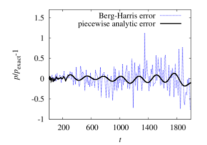
Figure 14: The relative error in the piecewise-analytic method applied to $100,000$ samples drawn from the first passage time distribution of Sec. VI.3, compared to the relative error in the Berg-Harris method. The errors are defined here as the deviation from the exact result.

In this paper, a method to obtain smooth analytical estimates of probability densities, radial distribution functions and potentials of mean force in a statistically controlled fashion without using histograms was presented. This method only uses direct samples of data (distance samples in the case of radial distribution functions). Since this method is expected to be generally useful, we have made our implementation, coded in c and c++, available on the web.footnote4

While the method is based on the Berg-Harris method, the statistical criterion used in that method is most sensitive to the most common samples, which for radial distribution functions are not the ones of physical interest. To make the method work for radial distribution functions, a weighted resampling of this data was required. Spurious oscillations, allowed by the statistical noise, were eliminated using a piecewise approach. In addition, one can optionally patch the piecewise-analytic form to avoid discontinuities within the errors, if desired. The resampled, piecewise smoothing method was demonstrated on data from event-driven DMD simulations of water, and proved to give a much smoother result than the histogram method.

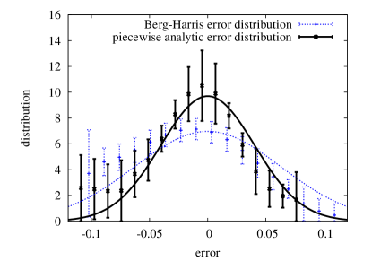
Figure 15: The distribution of the relative errors in the piecewise-analytic method applied to $100,000$ samples drawn from the first passage time distribution of Sec. VI.3, compared to the distribution of the relative error in the Berg-Harris method. The errors are defined here as the deviation from the exact result. The points with error bars are found by applying the piecewise analytic method to the deviations plotted in Fig. 14 (with errors from the jackknife procedure), while the drawn lines are fits to Gaussians with a zero mean.

If the purpose of a simulation is just to get a good smooth result for the radial distribution functions of a water model, one could use the histogram method with longer simulation runs to reduce the statistical uncertainties to some predetermined limit. However, the histogram would still be biased and known just at a lattice of points if a uniform bin size is used. To get a smoother and less biased curve from the histogram, one would also have to decrease the bin size by hand. The piecewise analytic method makes such tuning unnecessary. The method also make much longer runs unnecessary, since what appears to be very poor statistics for the histogram method turns out to be quite reasonable statistics for the piecewise analytic method. Remember that the same set of inter-atom distance are used in both methods. Apparently, there is much more statistics in the sample than the histogram is using (something that Berg and Harris also noticedBergHarris08 ).

For the test case considered here, the computational cost of doing longer runs is not that large, so the advantages of the piecewise analytic method may seem to be nice but not necessary. In other applications, however, such as in studies of the distribution of water molecules near a polymer or a bio-molecule (or near one of their polymer units), better statistical information is costly to obtain because such systems are not only computationally more demanding, but there are far less samples available in a single configuration since only the water molecules near the polymer or the bio-molecule are involved. The simulation run times would have to be much larger to compensate for this poor statistics, if histograms are used. In such cases, the piecewise analytic method is expected to be advantageous since it appears able to use more of the information present in the inter-particle distance sample.

The piecewise analytic method yields a smooth approximation to the probability density function, and the deviations of the empirical distribution from this smooth curve are supposed to be due to statistical noise. If this is true and the methods are unbiased, then for large enough sample size $n$, one would expect the distribution of errors in the probability density functions to be Gaussian with a zero mean. To test whether this is the case, the probability densities of the relative errors plotted in Fig. 14 were determined, both for the Berg-Harris and for the piecewise analytic method.footnote5 The results are shown in Fig. 15. Within statistical uncertainty, both distributions were found to be unbiased. Furthermore, for the piecewise analytic results, the error densities are roughly Gaussian. The errors from the Berg-Harris method, on the other hand, seem to show deviations from Gaussian behavior. The non-Gaussian nature of the errors of the Berg-Harris method might be due to the fact that the sample noise is fitted too closely since a large number of Fourier modes are necessary, which means the distribution of errors follows the distribution of the finite sample-size errors rather than being truly random. The Gaussian nature of the errors in the piecewise analytic method might be a confirmation that in the smooth approximation, enough Fourier modes have be taken into account for the remainder to be due to a random statistical noise.

One of the nice features of the piecewise analytic method is that one does not have to choose a bin size a priori, as one has to do in the histogram method. It is nonetheless true that within the smoothing method, one is to some extent free to choose the cut-off value $Q_{\mathrm{cut}}$ of the ‘quality’ parameter $Q$ and the maximum number $m_{\mathrm{max}}$ of basis functions allowed in the expansion of each interval. Note that both $Q_{\mathrm{cut}}$ and $m_{\mathrm{max}}$ are dimensionless numbers, and do not contain physical parameters, in contrast to the bin size parameter required in the histogram approach. Setting $Q_{\mathrm{cut}}$ too low may result in a bad fit to the data, while setting $m_{\mathrm{max}}$ too large may result in noise fitting and artificial oscillations. We have found that $Q_{\mathrm{cut}}\approx 0.6$ and $m_{\mathrm{max}}\approx 14$ are reasonable choices, and these values were used in all the applications presented above.

There is also some freedom in the choice of the set of basis functions, as long as they form a complete set. The Fourier basis used here is convenient and familiar, but others are possible. For instance, in Ref. VanZonetal08b, , a Chebyshev expansion was used. This expansion was chosen over the Fourier expansion because it gave fewer oscillations. The piecewise approach present in this paper, however, resolves the oscillation problem as well, and is expected to be less sensitive to the choice of basis functions than the original Berg-Harris method. Furthermore, the method was shown to also be applicable to other potentials of mean force and other probability densities with a hard-to-fit character.

- (1) D. A. McQuarrie, Statistical Mechanics (Harper Collins Publishers, 1976).
- (2) D. Frenkel and B. Smit, Understanding molecular simulation: From Algorithms to Applications (Academic Press, San Diego, 2002).
- (3) H. J. C. Berendsen, Simulating the Physical World: Hierarchical Modeling from Quantum Mechanics to Fluid Dynamics (Cambridge University Press, Cambridge, UK, 2007).
- (4) B. A. Berg and R. C. Harris, Comp. Phys. Comm. 179, 443 (2008).
- (5) R. van Zon, L. Hernández de la Peña, G. H. Peslherbe, and J. Schofield, Phys. Rev. E 78, 041103 (2008).
- (6) T. Gericke, P. Würtz, D. Reitz, T. Langen, and H. Ott, Nature Physics 4, 949 (2008).
- (7) L. Mones, P. Kulhánek, I. Simon, A. Laio, and M. Fuxreiter, J. Phys. Chem. B 113, 7867 (2009).
- (8) Y. Liu and T. Ichiye, J. Phys. Chem. 100, 2723 (1996).
- (9) A. Chandra and T. Ichiye, J. Chem. Phys. 111, 2701 (1999).
- (10) M.-L. Tan, J. T. Fisher, A. Chandra, B. R. Brooks, and T. Ichiye, Chem. Phys. Lett. 376, 646 (2003).
- (11) C. J. Fennell and J. D. Gezelter, J. Chem. Phys. 120, 9175 (2004).
- (12) R. van Zon and J. Schofield, J. Chem. Phys. 128, 154119 (2008).
- (13) L. Hernández de la Peña, R. van Zon, J. Schofield, and S. B. Opps, J. Chem. Phys. 126, 074105 (2007).
- (14) L. Hernández de la Peña, R. van Zon, J. Schofield, and S. B. Opps, J. Chem. Phys. 126, 074106 (2007).
- (15) R. van Zon and J. Schofield, J. Comp. Phys. 225, 145 (2007).
- (16) E. C. Cyr and S. D. Bond, J. Comput. Phys. 225, 714729 (2007).
- (17) A. B. Adib and C. Jarzynski, J. Chem. Phys. 122, 14114 (2005).
- (18) J. E. Basner and C. Jarzynski, J. Phys. Chem. B 112, 12722 (2008).
- (19) W. H. Press, S. A. Teukolsky, W. T. Vetterling, and B. P. Flannery, Numerical Recipes in Fortran, The Art of Scientific Computing (Cambridge University Press, Cambridge, UK, 1992), 2nd ed.
- (20) Alternatively, one can use other tests such as the Kuiper test, but these are less convenient for the piecewise approach presented later, since they involve several “hard-to-fit” points.
- (21) M. A. Stephens, J. Royal Stat. Soc. B 32, 115 (1970).
- (22) B. Efron, The Annals of Statistics 7, 1 (1979).
- (23) H. R. Künsch, The Annals of Statistics 17, 1217 (1989).
- (24) Another good explanation of the sensitivity of the K-S test to values near the median can be found in Ref. NumRecipes, , Ch. 4, Sec. 3.
- (25) One could imagine performing the reweighting at the level of K-S test instead, but this would modify the statistic. The problem is that it would then not be known what a reasonable testing criterion for this new statistic should be, or even whether it allows a simple formulation such as .
- (26) A procedure in which the piecewise Fourier series is restricted to be continuous across the interval boundaries was also considered but found to lead to undesirable oscillations near discontinuities, reminiscent of the Gibbs phenomenon.Jeffreys
- (27) H. Jeffreys and B. S. Jeffreys, Methods of Mathematical Physics (Cambridge University Press, Cambridge, UK, 1956), 3rd ed.
- (28) S. Redner, A Guide to First-Passage Processes (Cambridge University Press, Cambridge, UK, 1991).
- (29) This is the Laplace inverse of Eq. (6.4.8) in Ref. Redner, .
- (30) http://www.chem.utoronto.ca/~rzon/Code.html.
- (31) This analysis was also attempted for the deviations plotted in Fig. 12 but the error bars on the resulting distributions were too large to tell whether they are biased or non-Gaussian.