Instability and Nonlinear Evolution of Narrow-Band Directional Ocean Waves

Abstract

The instability and nonlinear evolution of directional ocean waves is investigated numerically by means of simulations of the governing kinetic equation for narrow-band surface waves. Our simulation results reveal the onset of the modulational instability for long-crested wave-trains, which agrees well with recent large-scale experiments in wave-basins, where it was found that narrower directional spectra leads to self-focusing of ocean waves and an enhanced probability of extreme events. We find that the modulational instability is nonlinearly saturated by a broadening of the wave-spectrum, which leads to the stabilization of the water-wave system. Applications of our results to other fields of physics, such as nonlinear optics and plasma physics are discussed.

Giant freak waves, or rogue waves, have been observed in mid-ocean and coastal waters Kharif03 , in optical systems Solli07 , and in parametrically driven capillary waves Shats10 . The freak/rogue waves are short-lived phenomena appearing suddenly out of normal waves, and with a small probability Akhmediev09 . The study of extreme gravity waves on the open ocean has important applications for the sea-faring and offshore oil industries, where they may lead to structural damage and injuries to personnel Kharif03 . It is, therefore, very important to understand the physical mechanisms that lead to the formation of freak waves. Since the linear theory cannot explain the number of extreme events that occur in the ocean and in optical systems, one has to account for nonlinear effects (e.g. wave-wave interactions) in combination with the wave dispersion. This can lead to the modulational instability (for water waves called the Benjamin-Feir instability Benjamin67 ; Ruban07 ), followed by focusing and amplification of the wave energy.

Wind-driven waves on the ocean often have wide frequency spectra that are peaked in the direction of the wind JONSWAP ; Mitsuyasu75 ; Hasselmann80 . The statistics of directional spectra for narrow-band gravity waves have also recently been studied experimentally in water basins Onorato09 ; Onorato09b ; Waseda09 , where it was found that sea states with narrow directional spectra (long–crested waves) were more likely to produce extreme waves. Examples of statistical models that govern collective interactions of groups of water waves are Hasselmann’s model Hasselmann62 for random, homogeneously distributed waves and Alber’s model Alber78 for narrow-banded wave trains. Wave-kinetic simulations in one spatial dimension have shown Landau damping and coherent structures Onorato03 , and recurrence phenomena Stiassnie08 for random water wave fields. In this Letter, we derive a nonlinear wave-kinetic (NLWK) equation for gravity waves in $2+2$ dimensions (two spatial dimensions and two velocity dimensions) and carry out simulations to study the stability and nonlinear spatio-temporal evolution of narrow-band spectra waves that were observed in the recent experiments by Onorato and coworkers Onorato09 . The present NLWK model, which is similar to Alber’s model Alber78 , is particularly suitable for studying the nonlinear dynamics of narrow-band water waves due to its relative simplicity. Similar nonlinear wave-kinetic equations also appear in the description of optical systems, photonic lattices, and plasmas Bingham97 .

Deep water gravity waves are governed by the dispersion relation $\omega=\sqrt{gk}$, where $g$ is the gravitational constant, $k=\sqrt{k_{x}^{2}+k_{y}^{2}}$ is the modulus of the wave vector ${\bf k}=k_{x}\widehat{\bf x}+k_{y}\widehat{\bf y}$, and $\widehat{\bf x}$ and $\widehat{\bf y}$ are the unit vectors in the $x-$ and $y-$directions. Assuming surface displacements of the form $\eta=(1/2)A({\bf r},t)\exp(-i\omega_{0}t+ik_{0}x)$+ complex conjugate, where $A$ is the slowly varying ($|\partial/\partial t|\ll\omega_{0}$, $|\nabla|\ll k_{0}$) envelope, ${\bf r}=x\widehat{\bf x}+y\widehat{\bf y}$ is the spatial coordinate, and $\omega_{0}=\sqrt{gk_{0}}$, the nonlinear interaction of water waves is governed by the nonlinear Schrödinger equation (NLSE)

$$i\left(\frac{\partial A}{\partial t}+v_{gr}\frac{\partial A}{\partial x}\right)+D_{x}\frac{\partial^{2}A}{\partial x^{2}}+D_{y}\frac{\partial^{2}A}{\partial y^{2}}-\xi|A|^{2}A=0,$$ (1)

where $v_{gr}=\partial\omega/\partial k_{x}=\omega_{0}/2k_{0}$ is the group velocity, $D_{x}=(1/2)\partial^{2}\omega/\partial k_{x}^{2}=-\omega_{0}/8k_{0}^{2}$ and $D_{y}=(1/2)\partial^{2}\omega/\partial k_{y}^{2}=\omega_{0}/4k_{0}^{2}$ are the group dispersion coefficients, and the nonlinear coupling coefficient is $\xi=\omega k_{0}^{2}/2$. Introducing the two-dimensional Wigner transform Moyal

$$f({\bf r},{\bf v},t)=\frac{1}{2(2\pi)^{2}}\int A^{*}({\bf R}_{+},t)A({\bf R}_{-},t)e^{i{\boldsymbol{\lambda}}\cdot({\bf v}-v_{gr}\widehat{\bf x})}\,d^{2}\lambda,$$ (2)

where we have denoted ${\bf R}_{\pm}={\bf r}\pm{\bar{\bar{\bf D}}}\cdot{\boldsymbol{\lambda}}$ and ${\bar{\bar{\bf D}}}\cdot{\boldsymbol{\lambda}}=D_{x}\lambda_{x}\widehat{\bf x}+D_{y}\lambda_{y}\widehat{\bf y}$, we obtain the evolution equation for the pseudo-distribution function $f$ as

$$\begin{split}\frac{\partial f}{\partial t}&+{\bf v}\cdot\nabla f-\frac{2i\xi}{(2\pi)^{2}}\int\int[I({\bf R}_{+},t)-I({\bf R}_{-},t)]\\ &\times~{}f({\bf r},{\bf v}^{\prime},t)e^{i{\boldsymbol{\lambda}}\cdot({\bf v}-{\bf v^{\prime}})}d^{2}v^{\prime}\,d^{2}\lambda=0,\end{split}$$ (3)

where $I({\bf r},t)=\int f({\bf r},{\bf v},t)\,d^{2}v$ is the variance of the surface displacement (the wave intensity). The transformation (2) between (1) and (3) is valid in both directions for a deterministic wave-train (corresponding to a “pure state” in quantum mechanics), with some restrictions on the distribution function $f$ Moyal ; however, we are interested in the statistical properties of an ensemble of waves, and more general choices of $f$ where the deterministic picture is abandoned Alber78 . In the absence of the nonlinear term in the left-hand side of (3), we have ${\partial f}/{\partial t}+{\bf v}\cdot\nabla f=0$, which dictates that the wave energy propagates in space with the group velocity ${\bf v}$. Our model is valid for waves with ${\bf v}\approx v_{gr}\widehat{\bf x}$. The dispersive properties of the wave are important for the nonlinear wave-wave interactions between wave-packets that are modeled by the interaction integral in the last term in the left-hand side of (3).

The velocity distribution can be related to the wave spectrum in frequency domain. Similar to Ref. Onorato09 , we will use the model spectrum parameterized by the Joint North Sea Wave Project (JONSWAP) as JONSWAP

$$S(\omega)=\frac{\alpha_{P}g^{2}}{\omega^{5}}\exp\left(-\frac{5}{4}\frac{\omega_{p}^{4}}{\omega^{4}}\right)\gamma^{\exp\left[-\frac{(\omega-\omega_{p})^{2}}{2\sigma^{2}\omega_{p}^{2}}\right]},$$ (4)

where $\omega_{p}$ is the peak frequency, $\gamma$ is the peak enhancement parameter and $\alpha_{P}$ is the Phillips parameter. Here $\gamma$ is in the range 1–6 for ocean waves Onorato09 , while $\alpha_{P}$ is in the range $0.0081$–$0.1$; the values $\gamma=1$ and $\alpha_{P}=0.0081$ gives the spectrum of fully developed wind seas Pierson64 , while the larger values are observed in water tank experiments. We will use $\alpha_{P}\approx 0.025$, $\gamma=3$ and $\sigma=0.08$, which are consistent with the Marintek water basin experiment in Refs. Onorato09 ; Onorato09b . Since the wave spectrum is concentrated around $\omega=\omega_{p}$, we will use $\omega_{0}=\omega_{p}$ and $k_{0}=k_{p}\equiv\omega_{p}^{2}/g$ in the evaluation of $D_{x}$ and $D_{y}$ in Eq. 3.

The integral of the spectrum (4) over all frequencies yields the variance of the surface elevation. While the variance of a monochromatic wave is $|A|^{2}/2$, from (2) we also have $\int f\,d^{2}v=|A|^{2}/2$. Hence, as initial conditions in our simulations, we will use $f=f_{0}({\bf v})=F_{0}(v)G(\theta)$ where we have introduced polar coordinates $v_{x}=v\cos(\theta)$ and $v_{y}=v\sin(\theta)$ in velocity space. We obtain $F_{0}$ from the frequency spectrum (4) by using the differential variance $dI=S(\omega)d\omega=F_{0}({v})\,vdv$, as

$$F_{0}(v)=S[\omega(v)]\frac{1}{v}\left|\frac{d\omega}{dv}\right|=S[\omega(v)]\frac{g}{2v^{3}},$$ (5)

where we used that the group speed $v$ of the wave packets is related to the wave frequency $\omega=\sqrt{gk}$ via $v={d\omega}/{dk}=\omega/2k=g/2\omega$, or $\omega(v)={g}/{2v}$. The directional spreading function is chosen as Mitsuyasu75 $G(\theta)=G_{0}\cos^{N}({\theta}/{2})=G_{0}{[1+\cos(\theta)]^{N/2}}/{2^{N/2}}$, where $\cos(\theta)=v_{x}/v$, $v=(v_{x}^{2}+v_{y}^{2})^{1/2}$, and $G_{0}$ is a normalization constant Mitsuyasu75 such that $\int_{-\pi}^{\pi}G(\theta)\,d\theta=1$. We note that $G$ has a maximum at $\theta=0$ and tends to a narrower distribution with an increase of the parameter $N$.

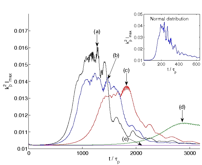
Figure 1: (Color online) The time-evolution of the maximum intensity $k_{p}^{2}I_{max}$ for (a) $N=840$ (black) (b) $N=200$ (blue), (c) $N=90$ (red), (d) $N=50$ (green), (e) $N=24$ (magenta), and the case of a narrow-band normal velocity distribution (the inset). The spatial distributions of wave intensity for (a)–(d) are shown in Fig. 3 at the times indicated here with arrows.

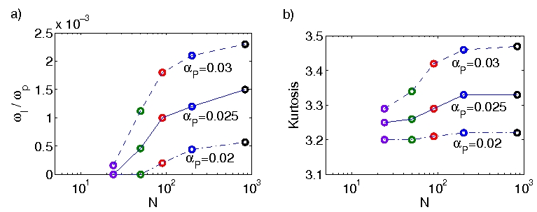
Figure 2: (Color online) a) The linear growth rate $\omega_{I}$ of the fastest growing wavemode and b) maximum kurtosis for $N=840$ (black) $N=200$ (blue), $N=90$ (red), $N=50$ (green), and $N=24$ (magenta), for $\alpha_{P}=0.02$ (dashed line), $\alpha_{P}=0.025$ (solid line) and $\alpha_{P}=0.03$ (dash-dotted line). The solid line ($\alpha_{P}=0.025$) corresponds to curves (a)–(e) in Fig. 1.

Equation (3) can be cast into a numerically more convenient form by employing the Fourier-transform in velocity space

$$\widehat{f}({\bf r},{\boldsymbol{\eta}},t)=2\int f({\bf r},{\bf v},t)e^{i{\boldsymbol{\eta}}\cdot{\bf v}}\,d^{2}v,$$ (6)

which transforms Eq. (3) into

$$\frac{\partial\widehat{f}}{\partial t}-i\nabla_{\boldsymbol{\eta}}\cdot\nabla\widehat{f}+2i\xi[I({\bf r}+{\bar{\bar{\bf D}}}\cdot{\boldsymbol{\eta}},t)-I({\bf r}-{\bar{\bar{\bf D}}}\cdot{\boldsymbol{\eta}},t)]\widehat{f}({\bf r},{\boldsymbol{\eta}},t)=0,$$ (7)

where $I=\widehat{f}({\bf r},{\boldsymbol{\eta}},t)_{{\boldsymbol{\eta}}={\boldsymbol{0}}}/2$. A similar equation was derived by Alber Alber78 , starting from the Davey-Stewartson equations for weakly nonlinear gravity waves. The numerical approximation of (7) is based on a method to solve the Fourier transformed Vlasov equation Eliasson02 . Using a pseudo-spectral method in space, the operator $\nabla$ is converted to multiplication by $i{\boldsymbol{\kappa}}$, and the spatial shifts by $\pm{\bar{\bar{\bf D}}}\cdot{\boldsymbol{\eta}}$ in Eq. (7) are converted to multiplications by $\exp[\pm i({\bar{\bar{\bf D}}}\cdot{\boldsymbol{\eta}})\cdot{\boldsymbol{\kappa}}]$, where ${\boldsymbol{\kappa}}$ is the wave vector. The system was solved in a computational window moving with the group speed of the peak wave. We used a spatial domain of size $L_{x}\times L_{y}=100\,k_{p}^{-1}\times 500\,k_{p}^{-1}$, resolved by $N_{x}\times N_{y}=32\times 32$ intervals and with periodic boundary conditions, and a Fourier transformed velocity domain $L_{\eta x}\times L_{\eta y}=160\pi v_{ph}^{-1}\times 160\pi v_{ph}^{-1}$ with $N_{\eta x}\times N_{\eta y}=80\times 80$ intervals, where $v_{ph}=\omega_{p}/k_{p}$ is the phase speed of the peak wave. The velocity domain in our simulations is thus $v_{x,min}\leq v_{x}\leq v_{x,max}$ and $v_{y,min}\leq v_{x}\leq v_{y,max}$ where $v_{x,min}=0$, $v_{x,max}=2\pi N_{\eta x}/L_{\eta x}=2v_{gr}$, and $-v_{y,min}=v_{y,max}=\pi N_{\eta y}/L_{\eta y}=v_{gr}$. The simulation was initialized with the JONSWAP spectrum, where the Fourier integral (6) was evaluated numerically to obtain the spectrum in $\boldsymbol{\eta}$ space. Random numbers of the order $10^{-2}$ of the initial intensity was added to the solution in order to seed the modulational instability. The initial conditions give an intensity of $I\approx 0.010\,k_{p}^{-2}$ uniformly distributed in space, which is compatible with the experiments of Onorato et al. Onorato09 . To compare with the experimental observations of Onorato et al. Onorato09 , we carried out simulations for $N=24$, $50$, $90$, $200$, and $840$ corresponding to the Marintek experiment in Ref. Onorato09 . They used $\omega_{p}=2\pi\,\mathrm{s}^{-1}$ (1 Hz) and corresponding $k_{p}=4.1\,\mathrm{m}^{-1}$, and a significant wave height $H_{s}=0.08\,\mathrm{m}$, giving a wave intensity of $I\approx 5\times 10^{-4}\,\mathrm{m}^{2}$.

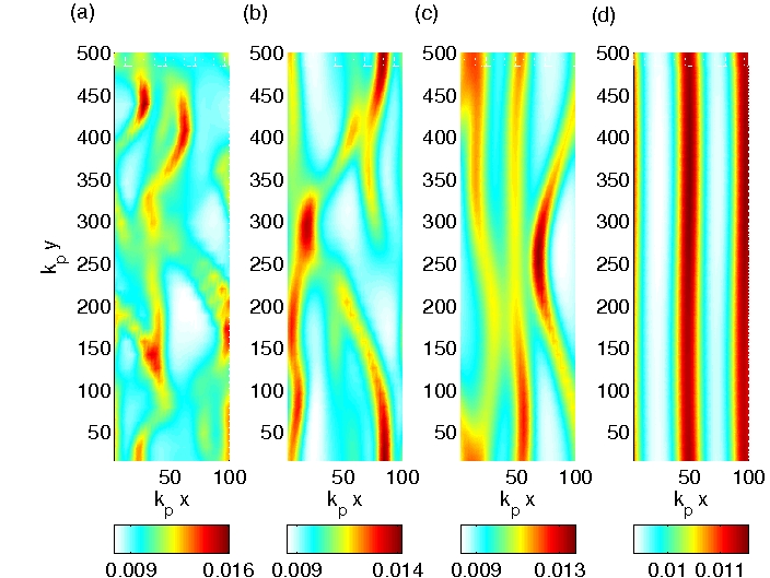
Figure 3: (Color online) The spatial distribution of the normalized wave intensity $k_{p}^{2}I$ for (a) $N=840$ at $t=1.27\times 10^{3}\,\tau_{p}$, (b) $N=200$ at $t=1.46\times 10^{3}\,\tau_{p}$, (c) $N=90$ at $t=1.81\times 10^{3}\,\tau_{p}$, and (d) $N=50$ at $t=2.90\times 10^{3}\,\tau_{p}$, corresponding to the curves (a)–(d) in Fig. 1.

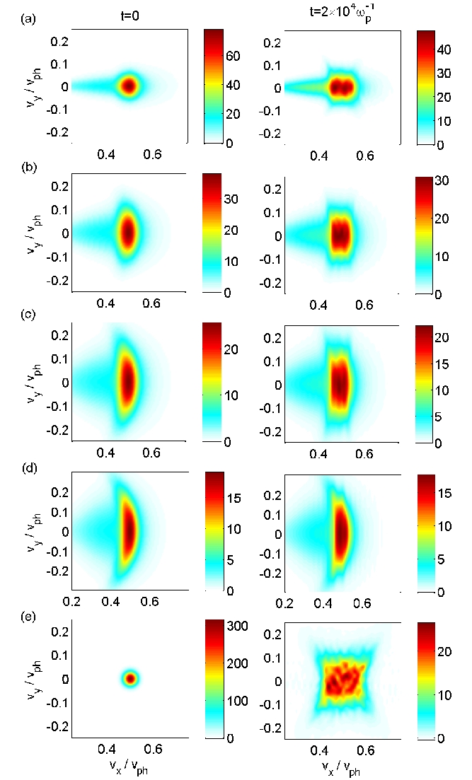
Figure 4: (Color online) The velocity distribution $\omega_{p}^{2}f$ of the wave energy, averaged over space, at $t=0$ (left column) and $t=3.2\times 10^{3}\tau_{p}$ (right column), for (a) $N=840$ (b) $N=200$, (c) $N=90$, (d) $N=50$. Panel (e) shows the narrow-band normal velocity distribution at $t=0$ (left) and $t=640\,\tau_{p}$ (right).

According to the analysis of Alber Alber78 , using a model two-dimensional normal spectrum, there are two conditions for the modulational instability: first, the modulational wavenumbers must lie within a certain directional range (in Alber’s case $|K_{x}|>\sqrt{2}|K_{y}|$ similar to the Benjamin-Feir instability), and second, the wave steepness (the wave amplitude multiplied by $k_{p}$) must be larger than the normalized (by the component of the spectral peak) spectral bandwidth. In our simulations, using directional JONSWAP spectra, we observed the modulational instability and the self-focusing of the wave energy into localized wave packets for $N$ larger than $24$. We measured the maximum value of the energy density in the simulation domain, and plotted its time evolution in Fig. 1 (the time is give in units of the peak wave period $\tau_{p}=2\pi/\omega_{p}$). Initially, there is an exponential growth phase, reminiscent of the Benjamin-Feir instability for monochromatic wave trains Benjamin67 . The modulational instability is fastest growing for $N=840$, and decreases with decreasing values of $N$. For $N=24$ we do not observe any instability. For modulationally unstable cases, the exponential growth phase is followed by a nonlinear saturation of the instability, and finally a decrease of the maximum energy density down to its initial background value $I\sim 0.01k_{p}^{-2}$, as seen in curves (a)–(d) of Fig. 1. The inset shows a simulation with a narrow-band normal distribution of the form $f=4\omega_{p}^{-2}\exp[-2(v_{y}^{2}+(v_{x}-v_{g}r)^{2})/\sigma^{2}]$ with $\sigma=0.04\,v_{ph}$, which yields the initial wave intensity $I=0.01k_{p}^{-2}$ that is similar as in curves (a)–(d). This case shows a rapidly growing instability to large amplitudes and then a decrease. The linear growth rate $\omega_{I}$ of the instability for different values of $N$ and $\alpha_{P}$ was measured from the data and plotted in Fig. 2(a). The growth rate is larger up to some limiting value for long-crested waves with $N>10^{2}$, while it approaches zero for smaller values of $N$. A growth rate of $\omega_{I}=1$–2$\times 10^{-3}\omega_{p}$ implies an amplitude doubling of the unstable wave in 50–100 wave periods. The growth rate is sensitive to changes of $\alpha_{P}$ and shows an increase/decrease of 50% with an increase/decrease of $\alpha_{P}$ by 20%; this is consistent with a ratio of unity between the wave steepness and the spectral bandwidth, so that the system is weakly unstable. The strongly unstable case for the narrow normal distribution has a growth rate $\omega_{I}\approx 0.008\omega_{p}$, which is close to the limiting value Alber78 $\omega_{I}=Ik_{p}^{2}\omega_{p}$ for monochromatic waves.

The kurtosis is traditionally Higgins63 estimated by the formula $\lambda_{4}=3+24k_{p}^{2}\sigma^{2}$, where $\sigma$ is the standard deviation of the surface elevation. (The factor 3 comes from the assumption of Gaussian statistics and the term $24k_{p}^{2}\sigma^{2}$ is a nonlinear correction to the Gaussian statistics.) Assuming that the wave field is ergodic, we have $\sigma^{2}=\langle I\rangle$, where $\langle I\rangle$ is the spatially averaged wave intensity. As noted in Ref. Onorato09b , this formula underestimates the kurtosis compared to the experimental values for narrow-band water waves, where an increase of the kurtosis was observed at later stages of the wave dynamics. Our model also conserves $\langle I\rangle$ and hence the formula predicts constant kurtosis. Taking into account that the wave-field is non-stationary and that the wave intensity varies in space (see Fig. 3), we, instead, estimate the kurtosis as $\lambda_{4}=3\langle I^{2}\rangle/\langle I\rangle^{2}+24k_{p}^{2}\langle I\rangle$, which assumes that the surface obeys Gaussian statistics locally everywhere. Using this estimate, we see in Fig. 2(b) that larger $N$ gives larger kurtosis, in good agreement with experimental observations Onorato09 ; Onorato09b ; Waseda09 . Figure 3 shows that the wave energy is concentrated into narrow bands, elongated along the $y$-direction, which are propagating from left to right with speeds close to $v_{gr}$. At later stages, the wave-packets start to break up due to the two-dimensionality in space and the elongated bands of wave energy become more and more wiggled with the appearance of obliquely propagating waves, similar to those observed in Ref. Ruban07 . For the modulationally unstable cases, the nonlinear interaction leads to a broadening of the distribution function in velocity space, as seen in Fig. 4. This, in turn, leads to a stabilization of the system via phase mixing of the wave envelopes Alber78 , and a saturation and decrease of the maximum intensity shown in Fig. 1.

To summarize, we have performed a series of kinetic simulations of narrow-banded water waves for different degrees of directional energy spectra. We observe an onset of the modulational instability and self-focusing of the wave energy for waves with narrow directional spectra, leading to an increase of the estimated kurtosis. The modulational instability saturates via the occurrence of narrow wave-packets, which later disperse due to the broadening of the wave spectrum. Our simulation results are in excellent agreement with observations from recent large-scale experiments in wave-basins Onorato09 ; Onorato09b ; Waseda09 .

References

- (1) C. Kharif and E. Pelinovsky, Eur. J. Mech. B/Fluids 22, 603 (2003).
- (2) D. R. Solli et al., Nature 450, 1054 (2007); A. Montina et al., Phys. Rev. Lett. 103, 173901 (2009); R. Höhmann et al., ibid. 104, 093901 (2010).
- (3) M. Shats et al., Phys. Rev. Lett. 104, 104503 (2010).
- (4) N. Akhmediev et al., Phys. Rev. A 80, 043818 (2009).
- (5) T. B. Benjamin and J. E. Feir, J. Fluid Mech. 27, 417 (1967).
- (6) V. P. Ruban, Phys. Rev. Lett. 99, 044502 (2007).
- (7) K. Hasselmann, J. Fluid Mech. 12, 481 (1962); ibid 15, 273 (1963).
- (8) I. E. Alber, Proc. R. Soc. Lond. A 363, 252 (1978).
- (9) M. Onorato et al., Phys. Rev. E 67, 046305 (2003).
- (10) M. Stiassnie et al., J. Fluid Mech. 598, 245 (2008).
- (11) K. Hasselmann et al., Dtsch. Hydrogr. Z. A8(Suppl.) No. 12 (1973).
- (12) H. Mitsuyasu et al., J. Phys. Oceanogr. 5, 750 (1975).
- (13) D. E. Hasselmann et al., J. Phys. Oceanogr. 10, 1264 (1980).
- (14) M. Onorato et al., Phys. Rev. Lett. 102, 114502 (2009).
- (15) M. Onorato et al., J. Fluid Mech. 627, 235 (2009).
- (16) T. Waseda et al., J. Phys. Oceanogr. 39, 621 (2009).
- (17) R. Bingham et al., Phys. Rev. Lett. 78, 247 (1997).
- (18) J. E. Moyal, Math. Proc. Cambridge Phil. Soc. 45, 99 (1949); T. Takabayasi, Prog. Theor. Phys. 11, 341 (1954).
- (19) W. J. Pierson, Jr. and L. Moskowitz, J. Geophys. Res. 69, 5181 (1964).
- (20) B. Eliasson, J. Comput. Phys. 181, 98 (2002).
- (21) M. S. Longuet-Higgins, J. Fluid Mech. 17, 459 (1963); N. Mori and P. A. E. M. Janssen, J. Phys. Oceanogr.36 1471 (2006).